Effects of Mainstream Velocity and Turbulence Intensity on the Sweeping Jet and Film Composite Cooling

Abstract

The jet always sweeps to the leftmost and rightmost points in the sweeping jet and film composite cooling (SJF) process, resulting in a different coolant flow in each film hole. The film can not easily cover the outer surface evenly under the scouring of the mainstream. This work presents a case study to analyze the effects of two mainstream variables on the film areodynamic and cooling performance of the SJF. Three different mainstream velocities (V_m = 10 m/s, 50 m/s, 90 m/s) and three different mainstream turbulence intensities (Tu = 1%, 10%, 20%) are discussed. Results indicate that the increase of mainstream velocity yields to better film attachment. When the mainstream velocity increases from 10 m/s to 50 m/s, the overall cooling effectiveness and total pressure loss coefficient are reduced by 17.68% and 98.60%, respectively. When the mainstream velocity increases from 50 m/s to 90 m/s, the overall cooling effectiveness and total pressure loss coefficient are almost unchanged. The effect of turbulence intensity on the overall cooling effectiveness and total pressure loss coefficient are relatively small. The increase of mainstream turbulence intensity enhances the disturbance of the mainstream to the coolant from the middle film holes, and the distribution of adiabatic film cooling effectiveness is more uneven when the mainstream turbulence intensity is raised to 10% and 20%. In the research scope of present work, the flow structure, total pressure loss coefficient and overall cooling effectiveness are the most expected under the conditions of lower turbulence intensity and higher mainstream velocity (Tu = 1%, V_m = 90 m/s).

1. Introduction

In the past decades, temperatures inside turbines have been increasing, and the leading edge cooling approaches have developed from the spanwise cylindrical convective cooling channel to jet and film composite cooling. Zhang et al. [1] and Wang et al. [2] studied the flow structure and heat transfer characteristics of “normal jet and film composite cooling” and “tangential jet and film composite cooling”. Their results show that the heat transfer coefficient distribution of a tangential jet on the impinging surface is more uniform than that of a normal jet, but the overall cooling effectiveness of the two kinds of composite cooling are basically the same. Regarding tangential jet cooling, compared with straight nozzles, helical nozzles can increase the velocity of the vortex in the impingement chamber, thus enhancing the heat transfer effectiveness of the impinging surface [3]. Besides, the fluidic oscillator has entered the public view because of its high-frequency sweeping jet and its ability to save the amount of coolant in the field of impingement cooling, and it also has the same advantages as the tangential jet; that is, the heat transfer coefficient of the impinging surface is relatively more uniform. The curved fluidic oscillator was invented by Bowles Fluidic Corporation in 1979 [4], and it is used for flow control [5], noise reduction [6], etc. Furthermore, the fluidic oscillator has been widely studied as a film cooling structure and impingement cooling structure over the past five years.

Regarding the sweeping jet film cooling section, Hossain et al. [7] believes that the transverse flow will not affect the sweep frequency. Moreover, compared with 777-shaped hole, the spanwise film momentum of the fluidic oscillator is small, and the film thickness of the fluidic oscillator is thinner than that of the 777-shaped hole, resulting in a wider spanwise coverage area and a greater average cooling effectiveness of the fluidic oscillator [8]. The aerodynamic losses of the two kinds of shaped holes are equivalent [9]. The position where the fluidic oscillator is used as the film hole is on the suction surface, and it can also be used as the impingement cooling structure at the leading edge.

There have been several studies conducted on the impingement cooling effectiveness of sweeping jets. The sweeping jet has a greater cooling effectiveness in open areas than in enclosed areas, when the impinging distance (ratio of H/D) is equal to 2 [10]. A stagnation zone (which refers to the area where the velocity of the jet on the impinging surface decreases to 0) appears when the H/D ratio is greater than 2, and whether the impingement chamber is changed does not affect cooling [11]. Cooling effectiveness in the stagnation zone decreases with an increase in the ratio of H/D, while the cooling effectiveness near the stagnation zone increases with an increase in the ratio of H/D [12]. Sweeping jets provide greater cooling effectiveness than normal jets when H/D is 4–5 [13]. It should be noted, however, that when the H/D is greater than 5, the cooling effectiveness of sweeping jets decreases due to the normal momentum of the impinging surface decreases rapidly, this results in the normal jets providing a greater cooling effectiveness than the sweeping jets in this scenario [14]. Kim [15] also investigated the impact of impinging surface curvatures on aerodynamic and cooling properties. According to these results, cooling effectiveness is affected by centrifugal force, which decreases the thickness of boundary layer, while turbulent kinetic energy increases. Accordingly, these findings support Hossain’s [16] findings that the middle curvature is more efficient at cooling effectiveness. Li et al. [17] used PIV (Particle Image Velocimetry) equipment to investigate how curvature affects the aerodynamic properties of sweeping jets. Curvature profoundly affects flow structure; in the presence of a curvature of 10D, the momentum of coolant distributes circumferentially and radially, producing a pair of powerful vortices near the jet core.

Although Hossain [18] applied sweeping jet and film composite cooling (SJF) to a guide vane perfectly, the research on this composite cooling structure is still lacking. Two mainstream variables are examined in this study to determine their effect on film flow characteristics and cooling effectiveness, a single fluidic oscillator is placed inside a semi-cylindrical model, and the semi-cylinder is equipped with nine film holes that serve as a unit for studies on SJF. The conjugate heat transfer method will be applied to investigate the flow structure and cooling effectiveness of the SJF at three different mainstream velocities (V = 10 m/s, 50 m/s, 90 m/s) and three different mainstream turbulence intensities (Tu = 1%, 10%, 20%).

2. Computational Method

CFD needs a lot of accurate hypotheses to closely simulate experimental and real-world conditions, and it was tried several times in the field of manufacturing, specifically in plastic injection, in cooling, and in fluid emulsion injection. Each work gave some reasonable ideas, such as a well-defined model of a nozzle design for combined use of MQL and cryogenic gas in machining, with more or less very accurate boundaries and conditions [19]. Xu et al. [20] used CFD to analyse the effects of nozzle section geometries on the performance of the annular multi-nozzle jet pump; however, it could be perfected using the above ideas, and the model was completed in references [21,22]. Therefore, the current work carefully defines the physical model of the sweeping jet and film composite cooling, carefully adjusts the mesh quality, gives accurate boundary conditions within the range of actual working conditions, and the error between the calculation results and the experimental results is reasonable.

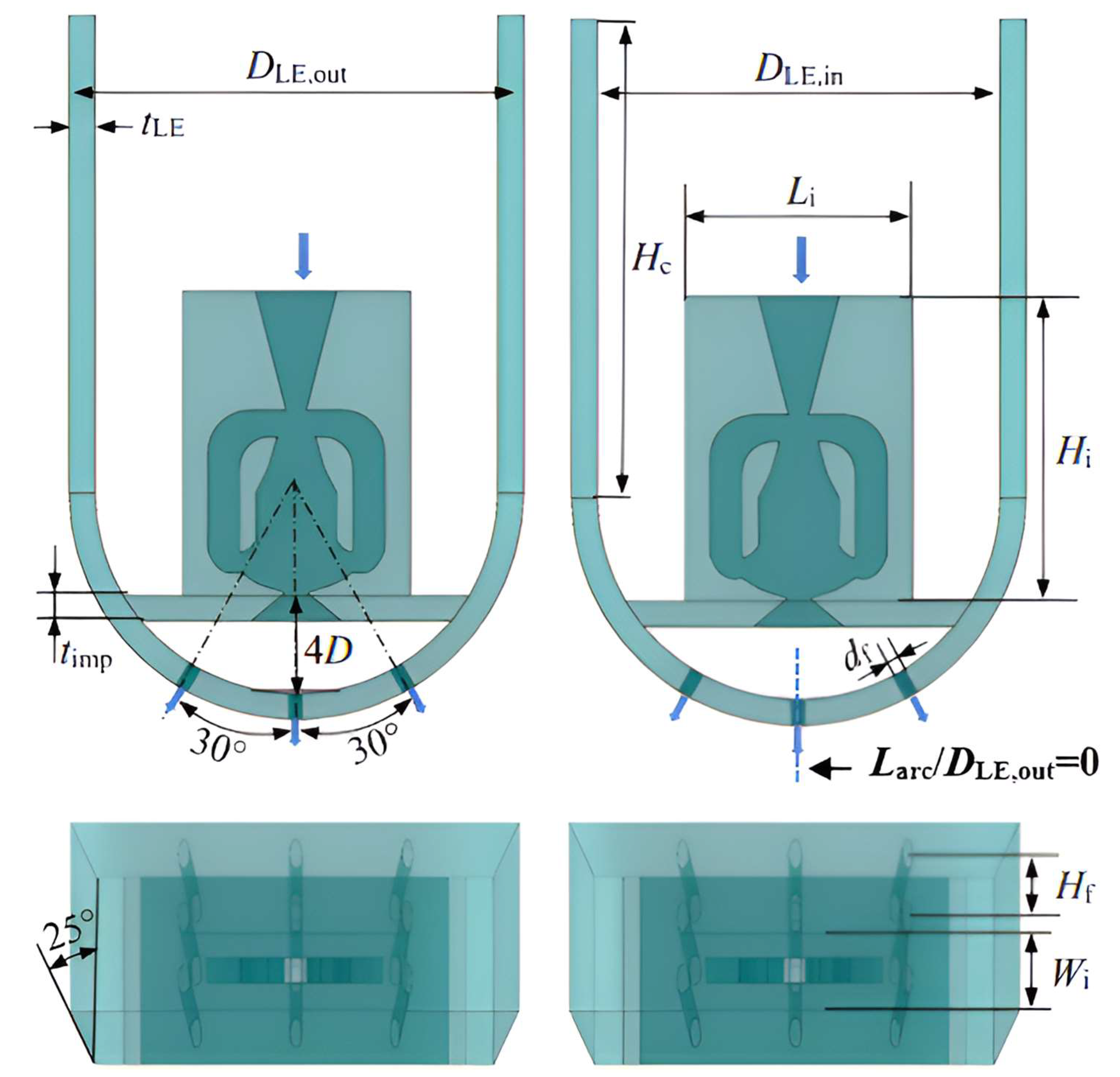
2.1. Physical Model of the SJF

The fluidic oscillator [4] is shown in Figure 1, and Figure 2 shows the geometric relationship throughout the SJF. The dimensionless impinging distance H/D = 4 in all working conditions of SJF. A total of 3 × 3 rows of film holes are arranged on the outer surface of the leading-edge model. The inclination angle of the film holes in the spanwise direction is 25°, so the spanwise angle between the inner surface and the outer surface of the semi-cylindrical model is 25°, which is equivalent to a cooling unit of the fluidic oscillator and film holes cut from the infinitely high blade. Besides, Figure 3 shows the whole calculation domain and location of the boundaries. A fluidic oscillator is filled with coolant, which impinges on the surface. Finally, it flows out of the leading-edge model through the film holes and protects the outer surface from the gas. The end of the semi-cylinder extends to simulate the body near the leading edge of the turbine blade.

Table 1. Dimensions of the SJF.

Dimension (mm)	D	df	DLE,in	DLE,out	tLE	timp	Hi	Li	Wi	Hc	Hf
Value	1.0	0.5	7.0	9.0	1.0	1.0	12.1	9.0	3.0	19.0	2.5

shows the geometrical dimensions of the SJF.

2.2. Governing Equations

Commercial software CFX 19.0 (CFX 19.0 is manufactured by Ansys Inc., which is located in Canonsburg, PA, USA) is employed for the current work. The three-dimensional compressible Unsteady Reynolds Averaged Navier–Stokes (URANS) equations and two-equations turbulence closure model are used for the simulations. High-order and second-order backward Euler methods are used for convection and time advance schemes. Since the compressible coolant is compressed and expanded in the fluidic oscillator, the compressibility of the fluid is taken into account. Therefore, the governing equations are as shown in Equations (1)–(3).

$$\frac{\partial \rho }{\partial t}+\frac{\partial }{\partial x_{\mathrm{j}}}\left(\rho U_{\mathrm{j}}\right)=0$$

(1)

$$\frac{\partial \rho U_{\mathrm{i}}}{\partial t}+\frac{\partial }{\partial x_{\mathrm{j}}}\left(\rho U_{\mathrm{i}}{U}_{\mathrm{j}}\right)=-\frac{\partial P}{\partial x_{\mathrm{i}}}+\frac{\partial }{\partial x_{\mathrm{j}}}\left[{\tau }_{\mathrm{ij}}-\rho \overline{u_{\mathrm{i}}{u}_{\mathrm{j}}}\right]$$

(2)

$$\frac{\partial \rho h_{\mathrm{t}}}{\partial t}-\frac{\partial P}{\partial t}+\frac{\partial }{\partial x_{\mathrm{j}}}\left(\rho U_{\mathrm{j}}{h}_{\mathrm{t}}\right)=\frac{\partial }{\partial x_{\mathrm{j}}}\left[\lambda \left(\frac{\partial T}{\partial x_{\mathrm{j}}}\right)-\rho \overline{u_{\mathrm{j}}h}\right]+\frac{\partial }{\partial x_{\mathrm{j}}}\left[U_{\mathrm{i}}\left({\tau }_{\mathrm{ij}}-\rho \overline{u_{\mathrm{i}}{u}_{\mathrm{j}}}\right)\right]$$

(3)

The energy equation of the solid domain for conjugating heat transfer simulation is given by:

$$\frac{\partial {\rho }_{\mathrm{s}}{c}_{\mathrm{Ps}}T}{\partial t}=\nabla \cdot \left({\lambda }_{\mathrm{s}}\cdot \nabla T_{\mathrm{s}}\right)$$

(4)

where U, u, ρ, P, τ_ij, h_t, c_Ps, T and λ are the velocity vector (m/s), velocity pulsation (m/s), density (kg/m³), pressure (Pa), stress tensor (kg/(m·s)), total enthalpy (J), the specific heat of the solid domain (J/(kg·K)), temperature (K), and thermal conductivity coefficient (W/(m·K)), respectively.

SST k-ω turbulence model is a two-equation model, which is composed of k-ω model which can solve the flow near the wall and k-ε model which can solve the free-stream flow outside the wall, given by:

$$\frac{\partial \left(\rho k\right)}{\partial t}+\frac{\partial \left(\rho U_{\mathrm{i}}k\right)}{\partial x_{\mathrm{i}}}=P_{\mathrm{k}}-{\beta }^{\ast }\rho k\omega +\frac{\partial }{\partial x_{\mathrm{i}}}\left[\left(\mu +{\sigma }_{\mathrm{k}}{\mu }_{\mathrm{t}}\right)\frac{\partial k}{\partial x_{\mathrm{i}}}\right]$$

(5)

$$\begin{array}{l}\frac{\partial \left(\rho \omega \right)}{\partial t}+\frac{\partial \left(\rho U_{\mathrm{i}}\omega \right)}{\partial x_{\mathrm{i}}}=\alpha \rho S^2-\beta \rho {\omega }^2+\frac{\partial }{\partial x_{\mathrm{i}}}\left[\left(\mu +{\sigma }_{\mathsf{\omega }}{\mu }_{\mathrm{t}}\right)\frac{\partial \omega }{\partial x_{\mathrm{i}}}\right]\\ +2\left(1-F_1\right)\rho {\sigma }_{\mathsf{\omega }2}\frac{1}{\omega }\frac{\partial k}{\partial x_{\mathrm{i}}}\frac{\partial \omega }{\partial x_{\mathrm{i}}}\end{array}$$

(6)

The turbulent eddy viscosity is used to closure the above two equations, given by:

$${\nu }_{\mathrm{t}}=\frac{a_{1}k}{\max \left(a_1\omega ,S{F}_2\right)}$$

(7)

In addition, some parameters in the two equations are given by:

$$P_{\mathrm{k}}=\min \left({\tau }_{\mathrm{ij}}\frac{\partial U_{\mathrm{i}}}{\partial x_{\mathrm{j}}},10\cdot {\beta }^{\ast }\rho k\omega \right)$$

(8)

$${\tau }_{\mathrm{ij}}=2{\nu }_{\mathrm{t}}{S}_{\mathrm{ij}}-\frac{2}{3}{\delta }_{\mathrm{ij}}k$$

(9)

$$S=\sqrt{2S_{\mathrm{ij}}{S}_{\mathrm{ij}}}\begin{array}{cc}& \end{array}{S}_{\mathrm{ij}}=\frac{1}{2}\left(\frac{\partial U_{\mathrm{i}}}{\partial x_{\mathrm{j}}}+\frac{\partial U_{\mathrm{j}}}{\partial x_{\mathrm{i}}}\right)$$

(10)

$$F_1=\tanh \left\{{\left\{\min \left[\max \left(\frac{\sqrt{k}}{{\beta }^{\ast }\omega y},\frac{500\nu }{y^2\omega }\right),\frac{4\rho {\sigma }_{\mathsf{\omega }2}k}{C{D}_{\mathrm{k}\mathsf{\omega }}{y}^2}\right]\right\}}^4\right\}$$

(11)

where F₁ is the blending coefficient, F₁ is equal to zero away from surface (k-ε model), and increases to one inside the boundary layer (k-ω model). y is the distance to the nearest wall.

$$C{D}_{\mathrm{kw}}=\max \left(2\rho {\sigma }_{\mathsf{\omega }2}\frac{1}{\omega }\frac{\partial k}{\partial x_{\mathrm{i}}}\frac{\partial \omega }{\partial x_{\mathrm{i}}},{10}^{-10}\right)$$

(12)

F₂ is the second blending coefficient and given by:

$$F_2=\tanh \left[{\left[\max \left(\frac{2\sqrt{k}}{{\beta }^{\ast }\omega y},\frac{500\nu }{y^2\omega }\right)\right]}^2\right]$$

(13)

All constants are computed by a blend from the corresponding constants of the k-ε and the k-ω model via α = α₁F + α₂ (1 − F) etc. The constants for this model are: α₁ = 5/9, α₂ = 0.44, β₁ = 3/40, β₂ = 0.0828, β* = 0.09, σ_k1 = 0.85, σ_k2 = 1, σ_ω1 = 0.5, σ_ω2 = 0.856.

2.3. Boundary Conditions

The mainstream and coolant are assumed to be air ideal gas, and the compressibility is emphatically considered. The inlet total temperature of the coolant and mainstream are set as 300 K and 600 K, respectively. The leading-edge model is based on the LS89 transonic blade of Von Kármán Lab [23], the blade inlet velocity is about 50 m/s; therefore, the mainstream inlet velocity of the leading edge model is set as 50 m/s. In the comparative study of sweeping jet and film composite cooling (SJF) and normal jet and film composite cooling (NJF) [24], the mass flow rate of the coolant is changed to make the blowing ratio between 1.05–4.11. However, the results show that when the blowing ratio is 4.11, the coolant in the middle film holes always flows to one side, and its flow direction does not change with time. Kong et al. [24] infer that the uneven pressure difference between the inlet and outlet of the film holes causes the airflow to flow to one side, and it will not easily flow to the other side again under the scouring of the mainstream. In order to verify this conclusion, the mainstream velocity is reduced from 50 m/s to 10 m/s and increased to 90 m/s, respectively. Similarly, the turbulence intensity is selected as 1%, 10%, and 20%, respectively, so the leading-edge model simulates the operation of the actual blade under wide conditions. The static pressure at the outlet is 101,325 Pa, and the turbulent intensity of coolant is 5% in all cases. Translational period boundaries are defined on the upper and lower surfaces of the calculation domain, interface boundaries are defined on the fluid and solid surfaces, and non-slip adiabatic walls are defined on all other surfaces. Except that the impinging surface is set as a constant wall temperature of 450 K, all the fluid domain walls in contact with the solid domain in the conjugate heat transfer scheme are set as adiabatic walls in the adiabatic scheme; therefore, the adiabatic scheme only has the fluid domain, and the other boundary conditions are the same as the conjugate heat transfer scheme.

Table 2. Boundary conditions used in the current work.

Total temperature of mainstream inlet, Tm/(K)	600
Velocity of Mainstream inlet, Vin,m/(m/s)	10, 50, 90
Static pressure of outlet, Pout/(Pa)	101,325
Total temperature of coolant inlet, Tc/(K)	300
Total pressure of coolant inlet, Pt,c/(Pa)	3.4 × 105
Mainstream inlet turbulence, Tuin,m/(%)	1, 10, 20
Coolant inlet turbulence, Tuin,m/(%)	5

shows the boundary conditions in detail. The simulations are convergent when the RMS residences of the mass, energy, and momentum conservation equations are less than 1 × 10⁻⁶.

2.4. Grid and Independence Test

The whole computational domain is divided into hexahedral meshes. Figure 4 shows the grid of the impinging surface and the fluidic oscillator. The height of 1st boundary layer is set as 1 × 10⁻⁷ m, which makes the Y+ less than 1 in all cases. The conditions of mainstream inlet velocity = 50 m/s and mainstream inlet turbulence = 1% are selected to test the grid independence. Three grid numbers (including 6.78 million, 9.48 million, and 11.43 million) are evaluated,

Table 3. An analysis of grid independence and its extrapolation value.

Element Number (Million)	Cp	Relative Error	ηov
6.78	3.59	1.508%	0.673
9.48	3.55	0.377%	0.689
11.43	3.54	0.094%	0.691
Extrapolation	3.53	-	0.692

presents the area-averaged OCE and the total pressure loss coefficient (C_p), which are based on the data collected from each grid, the extrapolation value was calculated by the Richardson method [25]. Markedly, the C_p and area-averaged OCE have relatively small errors, as the grid has 9.48 × 10⁶ elements. Thus, the grid that has 9.48 × 10⁶ elements is selected in the current work.

2.5. Parameter Definition

(1) The definition of cooling effectiveness is as follows:

$$\eta =\frac{T_{\mathrm{i}\mathrm{n},\mathrm{m}}-T_{\mathrm{o}\mathrm{w}}}{T_{\mathrm{i}\mathrm{n},\mathrm{m}}-T_{\mathrm{i}\mathrm{n},\mathrm{c}}}$$

(14)

where T_ow, T_in,m, and T_in,c are the outer surface temperature, total temperature of mainstream inlet, and total temperature of coolant inlet (K), respectively. In the conjugate heat transfer scheme, this formula calculates the OCE, and in the adiabatic scheme, this formula calculates the adiabatic film cooling effectiveness.

(2) To determine the flow penalty, the total pressure loss coefficient of a film-cooled turbine [26] is used. It is defined as follows:

$$C_P=\frac{\frac{m_{\mathrm{c}}}{m_{\mathrm{c}}+m_{\mathrm{m}}}{P}_{\mathrm{t},\mathrm{c},\mathrm{i}\mathrm{n}}+\frac{m_{\mathrm{m}}}{m_{\mathrm{c}}+m_{\mathrm{m}}}{P}_{\mathrm{t},\mathrm{m},\mathrm{i}\mathrm{n}}-P_{\mathrm{t},\mathrm{out}}}{P_{\mathrm{t},\mathrm{m},\mathrm{i}\mathrm{n}}-P_{\mathrm{out}}}$$

(15)

where m_m is mass flow of mainstream (kg/s), m_c is mass flow of coolant (kg/s), and the symbol P stands for pressure (Pa).

2.6. Turbulence Model Validation

A commercial software, CFX 19.0, was employed in the present work. Four turbulence models (including Standard k-ω, SST k-ω, Standard k-ε, and RNG k-ε) are selected for the current work. The sweep frequency and spanwise averaged Nu number are selected as the validation index, the experimental results of literatures [11,16] are selected as the reference.

Table 4. Comparison between turbulence models and experimental data.

Models	f/Hz
Exp. [16]	310
SST k-ω	315
Standard k-ω	353
RNG k-ε	270
Standard k-ε	254

indicates that the calculated data of the SST k-ω model is closest to the reference data. As depicted in Figure 5, in comparison with the other three models, the calculated data of SST k-ω model is agreement with the reference data well. The prediction results of the standard k–ω model significantly deviate from experimental results in the region of X/D < 4, and both the standard k–ε and RNG k–ε models overpredict the spanwise-averaged Nu number and underpredict the sweep frequency. Therefore, the SST k-ω turbulence model is employed in the current work.

3. Results

3.1. Aerodynamic Characteristics

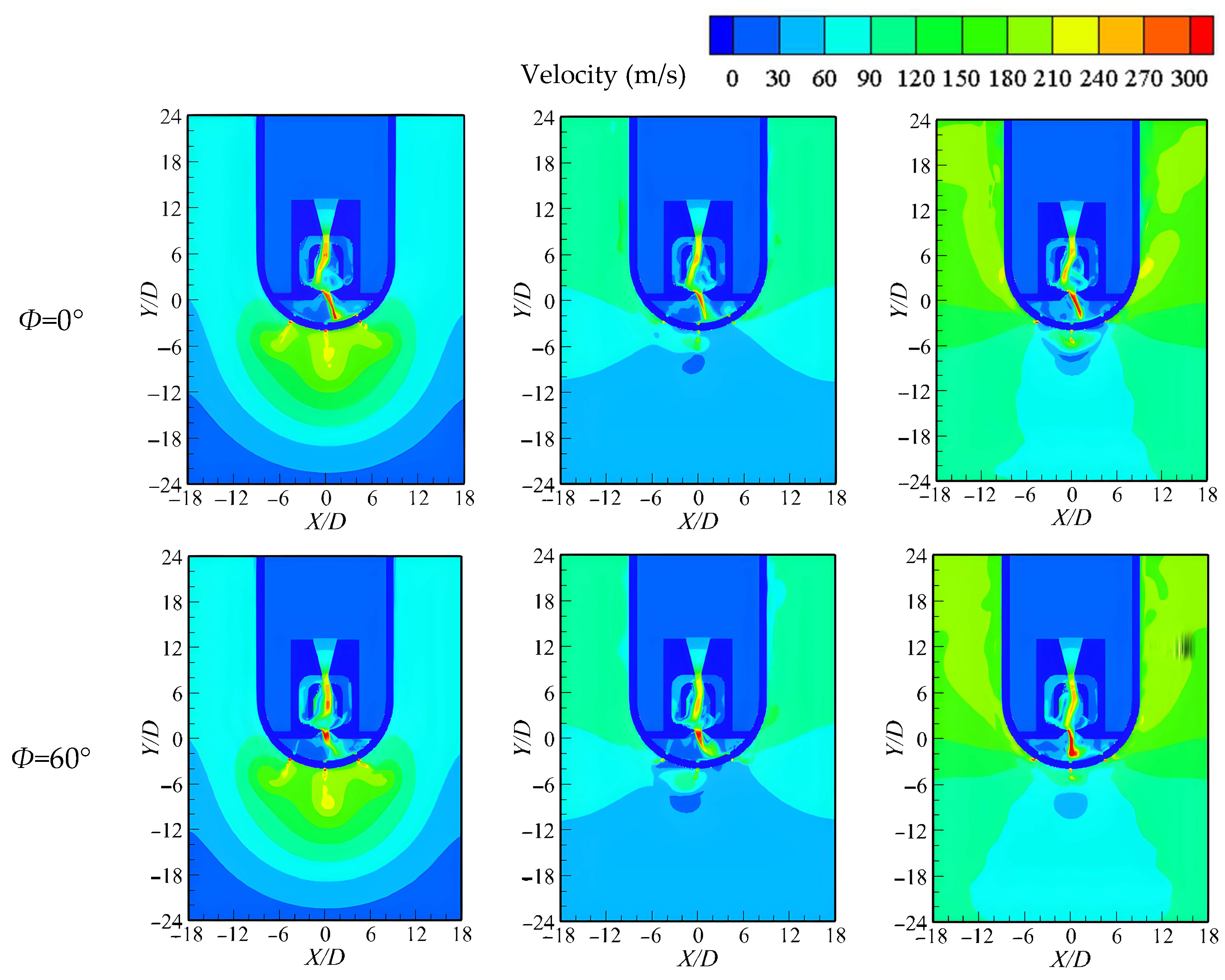
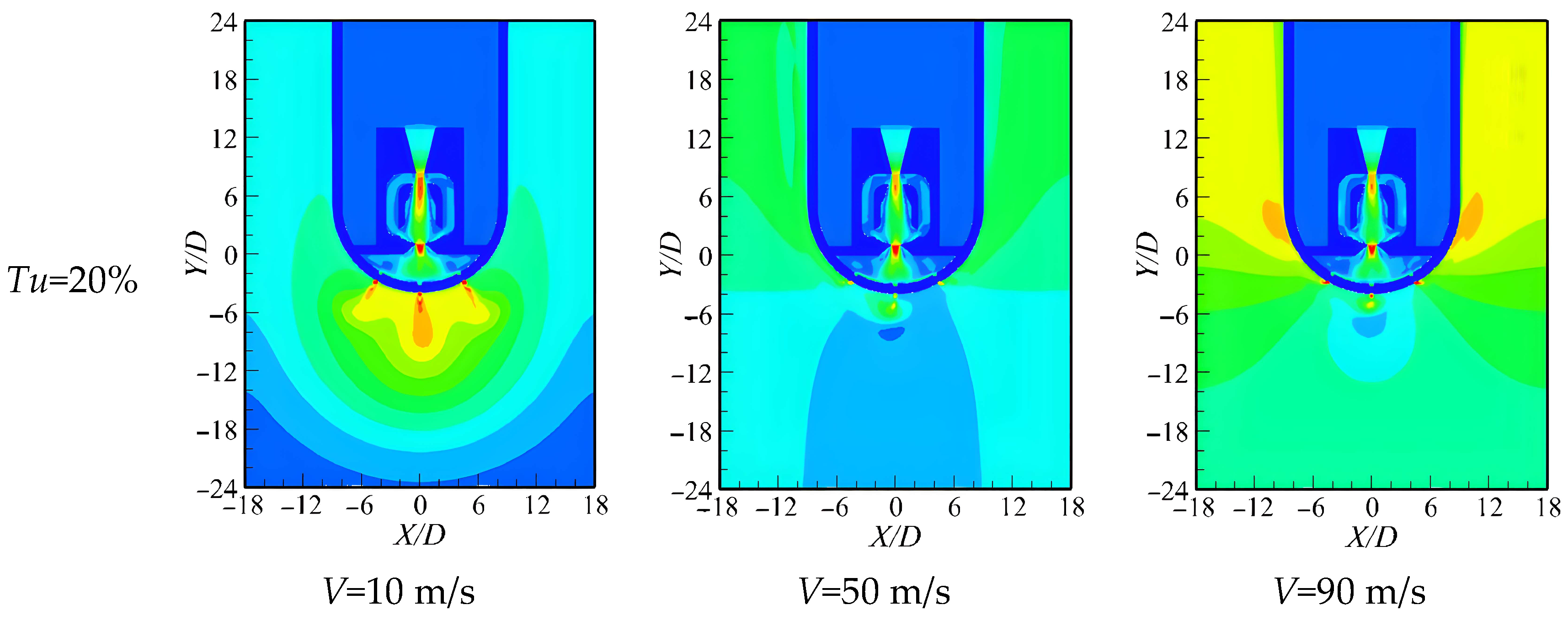
3.1.1. Velocity Contours of XY Section

Firstly, the instantaneous velocity distribution contours of the XY section under different mainstream velocities when the turbulence intensity is 1% is discussed. Since the mass flow of the coolant remains unchanged, the change of the internal flow field can be ignored, while the external flow field is obvious, so no streamline is drawn. Figure 6 depicts the instantaneous velocity distribution contours of XY section under different mainstream velocities. With a mainstream velocity of 10 m/s, the mainstream momentum is not sufficient to blow the film to the outer surface of the leading edge. A mainstream velocity of 50 m/s causes the coolant from the middle film holes (MFH) to flow to the left, entering a state called a “stalemate”. A mainstream velocity of 90 m/s brings the film close to the surface due to its large momentum. There is a certain effect that film pulsation will have on the external film cooling effectiveness under different phase angles for different velocity distribution contours.

Figure 7 shows the time-averaged velocity contours under three mainstream velocities and three mainstream turbulence intensities. It can be seen that the mainstream turbulence has little effect on the external flow field of the leading-edge model, and there are some slight differences. Obviously, the mainstream velocity has a great effect on the external flow field, which is mainly manifested in that with the increase of mainstream velocity, the film under the same turbulence intensity more easily sticks to the wall. When the mainstream velocity is 10 m/s, the flow field is symmetrical along the center line, but at this time, the film cannot adhere to the wall, resulting in severe mixing of the coolant and hot mainstream. When the mainstream increases to 50 m/s, the coolant in the MFH deflects to the left, and the mainstream scouring force is not enough to press the coolant flowing out of the MFH, therefore, the coolant flows along the positive pressure gradient. When the mainstream velocity increases to 90 m/s, the flow field is basically symmetrical along the middle line of the leading-edge model. At low turbulence, the flow field is strictly symmetrical along the middle line, this is because when the turbulence intensity of the mainstream is small, the high-speed flow gives a large and stable scouring force to the coolant, which makes the coolant from the MFH disperse evenly to both sides.

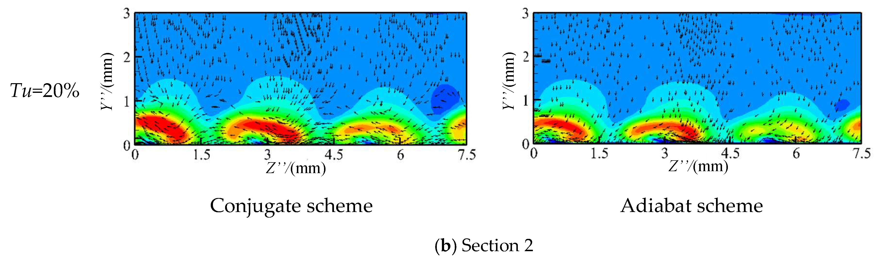
3.1.2. Flow Structure of Downstream of Left and Right Side Film Holes

As described in Figure 8, for further investigation of the mixing mechanism between coolant and mainstream, a spanwise section is arranged downstream of the rows of film holes with the relative positions of L_arc,out/D = ±6.5, with a 32.5° angle between the MFH, respectively. Because Section 1 and Section 2 are in the normal direction at different positions of the semi-cylinder, the global coordinates can not be used to face Section 1 and Section 2 squarely. Therefore, the local coordinates were set for Section 1 and Section 2, respectively, the relationship between the local coordinates and the global coordinates are shown in Equations (16)–(21). The working conditions with mainstream velocity of 50 m/s and turbulence intensity of 1% are taken for analysis.

$$X^{\prime }=X\cos \left(32.5\frac{\pi }{180}\right)+Y\sin \left(32.5\frac{\pi }{180}\right)$$

(16)

$$Y^{\prime }=-X\sin \left(32.5\frac{\pi }{180}\right)+Y\cos \left(32.5\frac{\pi }{180}\right)$$

(17)

$$Z^{\prime }=Z$$

(18)

$$X^{″}=X\cos \left(-32.5\frac{\pi }{180}\right)+Y\sin \left(-32.5\frac{\pi }{180}\right)$$

(19)

$$Y^{″}=-X\sin \left(-32.5\frac{\pi }{180}\right)+Y\cos \left(-32.5\frac{\pi }{180}\right)$$

(20)

$$Z^{″}=Z$$

(21)

In the same way, mapping the velocity component of global coordinates to local coordinates also requires Equations (16)–(21), and requires to change X, Y, Z, X′, Y′, Z′, X″, Y″, and Z″ to Vx, Vy, Vz, Vx′, Vy′, Vz′, Vx″, Vy″, and Vz″, respectively.

It can be seen from Figure 9 that the instantaneous velocity contours of Section 1 and Section 2 are always different under the same phase angle, which corresponds to the velocity distribution in Figure 6. Because the sweeping jet is periodically pulsating at different phase angles, the near wall velocities of Section 1 and Section 2 are always different. For Section 1, the low-speed area (blue) above the contours moves periodically with the phase angle, and the film velocity directly below the low-speed area is always the highest. When the Φ = 0°, the jet core is near the right film holes, the coolant flowing out of the left film hole is less affected by the jet core, and the coolant flowing out of the three left film holes is more uniform, at this time, the low-speed zone is at Z′ = 3.75. When Φ = 60° or 120°, by moving the end of jet core to the left film holes, the coolant is squeezed leftward, resulting in the imbalance of the outlet velocity of the three left film holes. The low-speed zone exists on both sides of Z′ = 3.75. When Φ = 180°, the jet core is at the left film holes, the film momentum is maxima at this point, and the blue low-speed zone is pushed to the range of Y′ > 3. In addition, the change of velocity distribution in Section 2 is small, because the coolant flowing out of the middle film flows in the direction of Section 1, and the coolant with higher mass flow makes the velocity pulsation here more intense.

Figure 10 shows the time-averaged velocity contours for Section 1 and Section 2 which are examined in relation to the mainstream velocity. These must be strongly mixed with the mainstream when the mainstream velocity is 10m/s, resulting in large mixing losses. There is a low-speed region at Y′ = 1 and Y′ = 2 (about 40 m/s) when the mainstream velocity is 50 m/s, which is the boundary between the mainstream and the film. Obviously, the velocity distribution of Section 1 and Section 2 is the most dissimilar. The boundary line of Section 1 is relatively flat, while the boundary line of Section 2 is relatively curved. This is because almost all the coolant flowing out of the MFH flows to Section 1. The coolant here has become relatively uniform after a series of spanwise diffusions. However, the film hole at Section 2 is not covered by the upstream film, and the boundary line at the exit of the film hole is higher, while it is lower at other positions. A mainstream velocity of 90 m/s causes the boundary between the mainstream and the film to move downward, causing some places to be close to the wall. Since the coolant from the MFH can flow evenly to both sides, Section 1 and Section 2 have relatively uniform velocity distributions.

The conjugate heat transfer scheme and adiabatic scheme under the conditions of mainstream velocity of 90 m/s, mainstream turbulence intensity of 1%, 10%, and 20% are selected to make the time-averaged velocity contours and velocity vector of Section 1 and Section 2. As shown in Figure 11a, compared with the results of the conjugate heat transfer scheme, the adiabatic scheme has similar flow structure and velocity distribution. With the increase of turbulence intensity, the overall change of the flow structure is small, and the low-speed region (90 m/s–100 m/s) gradually disappears. This shows that the strong pulsation of the mainstream makes its mixing with the film more intense, and increases the flow field velocity near the outer surface. The change of the velocity of Section 2 with turbulence in Figure 11b is the same. As mentioned above, the main difference between Section 1 and Section 2 is that the distribution shape of the mainstream and coolant buffer (110 m/s–120 m/s) is different. The external film cooling effectiveness is greatly affected by the coolant flowing out of the MFH since they tilt to the left, and Section 1’s buffer curve is gentler. The increase in turbulence intensity makes the coolant flowing out of the MFH tilt to the left more seriously as the coolant flows out of the MFH.

3.1.3. Total Pressure Loss Coefficient

The total pressure loss coefficient (C_p) is selected to investigate the effect of mainstream velocity and turbulence intensity on the aerodynamic loss in the conjugate heat transfer scheme.

Table 5. Total pressure loss coefficient and three important parameters under different mainstream velocities and turbulence intensities.

	Tu = 1%			Tu = 10%			Tu = 20%
	V = 10 m/s	V = 50 m/s	V = 90 m/s	V = 10 m/s	V = 50 m/s	V = 90 m/s	V = 10 m/s	V = 50 m/s	V = 90 m/s
mm (g/s)	1.6815	8.6017	16.6307	1.6806	8.6056	16.6218	1.6795	8.6027	16.7092
Pt,m,in (MPa)	1.0164	1.0455	1.1130	1.0166	1.0458	1.1446	1.0164	1.0458	1.1081
Pt,c,in (MPa)	3.6408	2.7622	3.6581	3.6561	2.8064	3.6538	3.6390	2.8064	3.6447
Cp	204.68	3.55	0.89	245.77	3.59	0.73	321.41	3.63	0.83

shows that the C_p under each turbulence intensity at the same velocity is within the calculation accuracy range, so the effect of turbulence intensity on the C_p can be ignored, but the C_p under different velocities at the same turbulence intensity differs by 1–2 orders of magnitude. The change of the coolant inlet total pressure (P_t,c,in) under different mainstream velocities is small, and because the mass flow of the coolant remains unchanged, the change of the aerodynamic loss in the fluidic oscillator, the impingement chamber and the film holes is small, and the change of the total pressure of the mainstream inlet (P_t,m,in) is also small. Therefore, it can be inferred that the main reason for the total pressure loss coefficient of 201.68–321.41 is the strong mixing between the mainstream and the coolant when the mainstream velocity is 10 m/s. When the mainstream velocity increases to 50 m/s and 90 m/s, the larger pressure of the mainstream makes the coolant flow close to the outer surface, the mixing loss between the coolant and the mainstream decreases, and the C_p decreases gradually. To sum up, when the mainstream inlet condition is 90 m/s and the turbulence intensity is 1%, the film has a better wall-attached flow phenomenon, and the coolant from the MFH flows evenly to both sides. Therefore, under this condition, the uniformity of film coverage on the outer surface and the C_p are more reasonable.

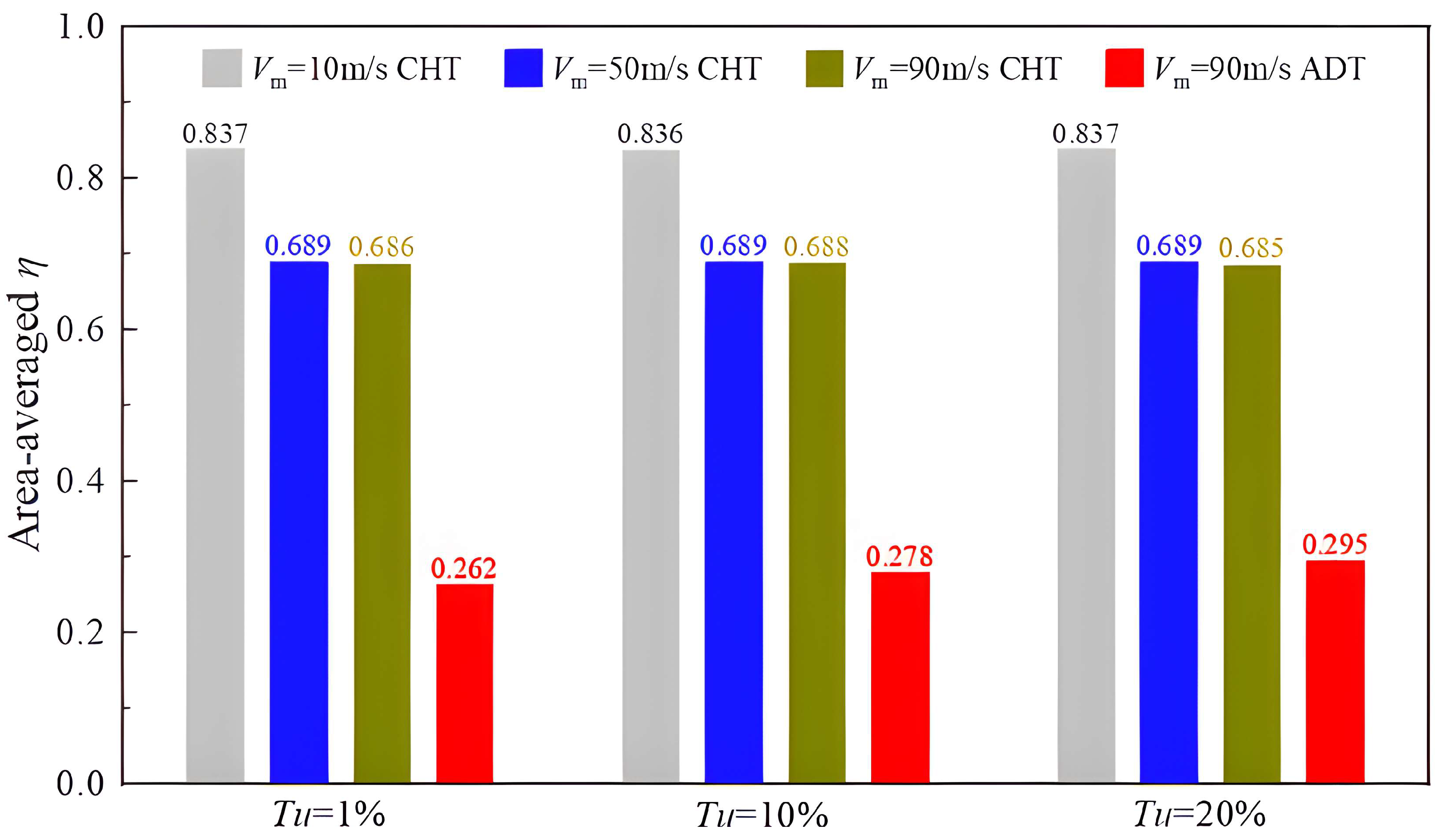
3.2. Heat Transfer Performance

Figure 12 shows the time-averaged contours of the OCE of the conjugate heat transfer scheme under different mainstream velocities and turbulence intensities. As shown in Figure 12, the mainstream turbulence intensity hardly affects the value and distribution of the OCE. When the mainstream velocity is 10 m/s, the OCE is the largest, but the mixing loss is large, but the C_p is 2–3 orders of magnitude higher than the other two velocities. Under the condition that the XZ velocity distribution is symmetrical along the line X/D = 0 (the velocity is 90 m/s and the turbulence intensity is 1%), the OCE is not strictly symmetrical. It is similar to the condition that the mainstream velocity is 50 m/s, and the higher OCE is distributed on the left edge of X/D = 0. A relatively small proportion of OCE comes from external film cooling, whereas about 70–80% comes from internal impingement cooling [27]. Therefore, the coverage of the film may only affect the distribution of the adiabatic film cooling effectiveness (η_ad).

The η_ad is taken as the evaluation index indicating the effect of mainstream turbulence intensity on the external cooling effectiveness, three working conditions with different turbulence intensities at the mainstream velocity of 90 m/s are selected for comparison. The η_ad can also be calculated by Equation (1), where T_ow is the temperature of the adiabatic outer wall. Figure 13 is the time-averaged cooling effectiveness contours under different turbulence intensities for conjugate and adiabat schemes, the OCE is about twice that of the η_ad under the same conditions, and its distribution is also roughly the same as that of the η_ad. Compared with the OCE, the distribution difference of the η_ad downstream of the film holes is more obvious, which reflects the coverage degree of the film on the outer surface to a certain extent; that is, the film in the blue area (η_ad = 0–0.2) is thin or even not covered by the film.

Furthermore, with the increase of turbulence intensity, the distribution of η_ad s becomes more and more uneven. As stated above, the mainstream turbulence intensities are selected as 1%, 10%, and 20% to prove that the unstable pressure difference between the inlet and outlet of the middle film holes is the main factor that causes the coolant to deflect to one side. Corresponding to Figure 7, at the mainstream velocity of 90 m/s, when the turbulence intensity is 1%, the coolant flowing from the middle film holes flows evenly to both sides. With the increase of the turbulence intensity, the disturbance of the mainstream to the coolant increases, and the coolant gradually flows to the left, and it does not easily flow to the other side again under the scouring of the mainstream, resulting in a higher adiabatic cooling effectiveness on the left than on the right. When the turbulence intensity reaches 20%, the disturbance of the mainstream to the coolant is the largest, the distribution of adiabatic cooling effectiveness on the left and right sides shows great differences. At the region of Z/D = −3 when the turbulence intensity is 10%, and at the region of Z/D = 1 when the turbulence intensity is 20%, the adiabatic cooling effectiveness of the left and right sides is more asymmetric. Referring to the literature on tangential jet and film composite cooling of semi-cylinders [1], the internal and external pressure of their middle film holes is extremely stable, but the problem of asymmetric cooling effectiveness on both sides of the middle film holes still occurs; thus, it can be inferred that this phenomenon is random in the current work.

Figure 14 is the comparison diagram of spanwise-averaged OCE under different mainstream velocities and turbulence intensities, the spanwise-averaged η_ad under different mainstream turbulence intensities at fixed mainstream velocities is also shown (When a series of spanwise lines are arranged at a certain distance from the outer surface, a series of spanwise-averaged cooling effectiveness is calculated). According to the cooling effectiveness curves at the same mainstream velocity in the Figure 14a–c, the turbulence intensity basically has no effect on the increase or decrease trend of OCE and η_ad. Under the same turbulence intensity, the spanwise-averaged OCE distribution is more uniform when the mainstream velocity is 10 m/s and 90 m/s in the conjugate heat transfer scheme. When the mainstream velocity is 50 m/s, the OCE on the left side of line L_arc/D_LE,out = 0 (L_arc represents the length of the curve moving along the outer surface of the semi-cylinder, starting from the intersection of the centerline and the outer surface of the semi-cylinder) is significantly higher than that on the right side, which proves once again that when the mainstream and the film are in a “stalemate”, the coolant always flow to the low pressure zone. The increase or decrease trend of OCE near the film holes is relatively gentle, which is caused by the heat conduction of the solid. The increase and decrease trend of the η_ad is obvious, and its maximum value is at L_arc/D_LE,out = 0, and then decreases rapidly to both sides. After passing through the film holes on both sides (L_arc/D_LE,out = ±6), it further increases and almost maintains a constant value until L_arc/D_LE,out = ±12. It should be pointed out that when the mainstream turbulence intensity is 1%, the difference of the η_ad between the region of 0 < L_arc/D_LE,out < 12 and −12 < L_arc/D_LE,out < 0 is small, and this difference increases with the increase of mainstream turbulence intensity.

As shown in Figure 15 below, the cooling effectiveness was further evaluated in relation to the average values of OCE and η_ad under various operating conditions. However, even though Figure 15 is the result of numerical calculation, it still has a certain reference value. Because in another work in the series of research on sweeping jets and film composite cooling (SJF), the overall cooling effectiveness of normal jets and film composite cooling (NJF) were carried out for experimental verification, the SST k-ω turbulence model can well predict the overall cooling effectiveness of NJF [24]. Additionally, Liu et al. pointed out that the SST k-ω turbulence model in the actual blade can also well predict the adiabatic cooling effectiveness of NJF [28]. The difference between SJF and NJF is only that the cylindrical normal jet hole is replaced by the sweeping jet hole (i.e., the fluidic oscillator), therefore, the SST k-ω turbulence model adopted in the current work can at least qualitatively explain the relative size of the overall cooling effectiveness and adiabatic cooling effectiveness under various conditions.

The turbulence intensity has little effect on the area-averaged OCE under the same mainstream velocity. In addition, the area-averaged OCE decreases by 17.68% when increasing the mainstream velocity from 10 m/s to 50 m/s; however, when the mainstream velocity increases from 50 m/s to 90 m/s, the area-averaged OCE hardly changes. Therefore, after the mainstream velocity reaches 50 m/s, the cooling capacity of the coolant has been fully developed, but combined with the distribution of spanwise-averaged OCE in Figure 14, the cooling effectiveness distribution is more reasonable when the mainstream velocity is equal to 90 m/s. Figure 15 also shows that the area-averaged η_ad increases by 12.59% when the turbulence intensity increases from 1% to 20%, the mixing of the mainstream and the film is small when the turbulence intensity is equal to 1%, and the ability of the mainstream to carry the coolant to the wall is low, the mainstream hardly disturbs the coolant flowing out of the MFH; the mixing between the mainstream and the film is intense when the turbulence intensity is equal to 10–20%, and the temperature of the film quickly approaches the temperature of the mainstream, resulting in the reduction of the η_ad, at this time. The mainstream has a large disturbance on the coolant flowing out of the MFH, making most of the coolant flow to the left, while the film in the right area of the MFH becomes thinner, and the strong mixing between film and the mainstream makes the η_ad here low, as shown in Figure 13. Therefore, the value of area-averaged η_ad cannot completely summarize the effect of turbulence intensity on external film cooling effectiveness. It can be seen from Figure 13 and Figure 14 that the effect of mainstream turbulence intensity on the η_ad is obviously regional. On the left side of L_arc/D_LE,out = 0, the η_ad increases with the increase of turbulence intensity, on the right side of L_arc/D_LE,out = 0, the η_ad decreases with the increase of turbulence intensity. The main reason for this result is that the disturbance of the mainstream turbulence intensity on the coolant from the MFH increases, resulting in most of the coolant flowing out of the MFH shifting to the left film holes, and a larger pressure from the mainstream will always force coolant to flow left through the MFH.

4. Conclusions

The sweeping jet in a conjugate heat transfer scheme and adiabatic scheme were numerically studied in a leading-edge model with film holes under different mainstream velocities and turbulence intensities. Flow structures and heat transfer characteristics were analyzed in detail and the conclusions are as follows.

As mainstream velocity approaches 10 m/s, the flow structure is less affected by turbulence intensity. However, when the mainstream velocity is higher, the flow structure is more sensitive to the turbulence intensity, which is mainly reflected in the gradual inclination of the coolant from the middle film hole to the left. The flow field structure is greatly affected by the mainstream velocity. The value of the mainstream velocity and the outlet velocity of the film holes determines the external flow structure and the C_p. When the turbulence intensity is 1% and the mainstream velocity is 10 m/s, the mainstream does not have enough momentum to push the film towards the outer surface. When the mainstream velocity is 50 m/s, the mainstream and the film are in the “stalemate” stage, and the coolant from the middle film holes (MFH) flows to the side with lower pressure. When the mainstream velocity is 90 m/s, the mainstream has enough momentum to push the film towards the outer surface. Currently, the coolant from the MFH flows to both sides evenly, and the mixing loss of mainstream and film is the lowest. However, the disturbance of the mainstream makes the coolant from the MFH tilt to the left again under higher turbulence intensity. Overall, the flow structure of the adiabatic scheme is basically the same as that of the conjugate heat transfer scheme.

The effect of mainstream velocity and turbulence intensity on the flow structure directly determines the OCE and the η_ad. The area-averaged OCE decreases by 17.68% when the mainstream velocity is increased from 10 m/s to 50 m/s. However, the area-averaged OCE changes little when the mainstream velocity increases from 50 m/s to 90 m/s. That is, the cooling capacity of the coolant has been fully developed after the mainstream velocity of 50 m/s. The expected C_p and OCE is achieved when the turbulence intensity is 1% and the mainstream velocity is 90 m/s in the range of the study. The change of turbulence intensity has little effect on the OCE, but the effect on the η_ad is obvious. On the left side of L_arc/D_LE,out = 0, the η_ad increases with the increase of turbulence intensity, and on the right side of L_arc/D_LE,out = 0, the η_ad decreases with the increase of turbulence intensity. The reason could be mainly attributed to the increasing of the disturbance of mainstream turbulence intensity on the film out of the MFH, which results in the flow deviation to the left.

The current work simulates the aerodynamic and heat transfer characteristics of SJF when it is applied to the leading edge of turbine blades under the conditions of mainstream velocity of 10 m/s, 50 m/s, 90 m/s and mainstream turbulence intensity of 1%, 10%, and 20%. This study suggests to designers that it has appropriate cooling effectiveness in a wide range of operating conditions when using SJF, and can provide a reference for changing the position of the middle film holes to avoid the uneven distribution of coolant on the leading-edge surface. In the future, the following work can be developed towards the global optimization algorithm with the aspect ratio, position, and number of film holes as independent variables. It is necessary to use experiments to verify the results of CFD to determine the accuracy of the research content.

References

1. Zhang, M.; Wang, N.; Han, J.-C. Overall effectiveness of film-cooled leading edge model with normal and tangential impinging jets. Int. J. Heat Mass Transf. 2019, 139, 577–587. [Google Scholar] [CrossRef]
2. Wang, J.; Li, L.; Li, J.; Wu, F.; Du, C. Numerical investigation on flow and heat transfer characteristics of vortex cooling in an actual film-cooled leading edge. Appl. Therm. Eng. 2021, 185, 115942. [Google Scholar] [CrossRef]
3. Pourmahmoud, N.; Zadeh, A.; Moutaby, O.; Bramo, A. CFD analysis of helical nozzles effects on the energy separation in a vortex tube. Therm. Sci. 2013, 16, 151–166. [Google Scholar] [CrossRef]
4. Stouffer, R.D. Oscillating spray device. U.S. Patent US4151955A, 1 May 1979. [Google Scholar]
5. Cerretelli, C.; Kirtley, K. Boundary Layer Separation Control With Fluidic Oscillators. J. Turbomach. 2009, 131, 041001. [Google Scholar] [CrossRef]
6. Raman, G.; Raghu, S. Miniature fluidic oscillators for flow and noise control-Transitioning from macro to micro fluidics. In Fluids 2000 Conference and Exhibit; American Institute of Aeronautics and Astronautics: Reston, VA, USA, 2000. [Google Scholar]
7. Hossain, M.A.; Agricola, L.; Ameri, A.; Gregory, J.W.; Bons, J.P. Sweeping Jet Film Cooling on a Turbine Vane. J. Turbomach. 2019, 141, 031007. [Google Scholar] [CrossRef]
8. Hossain, M.A.; Asar, M.E.; Gregory, J.W.; Bons, J.P. Experimental Investigation of Sweeping Jet Film Cooling in a Transonic Turbine Cascade. J. Turbomach. 2020, 142, 041009. [Google Scholar] [CrossRef]
9. Hossain, M.A.; Prenter, R.; Lundgreen, R.K.; Ameri, A.; Gregory, J.W.; Bons, J.P. Experimental and Numerical Investigation of Sweeping Jet Film Cooling. J. Turbomach. 2017, 140, 031009. [Google Scholar] [CrossRef] [Green Version]
10. Andrea, O.; Justin, H.; Husam, Z.; Erik, J.F.; Kapat, J.S. Impact of Sweeping Jet on Area-Averaged Impingement Heat Transfer. In Proceedings of the ASME Turbo Expo 2019: Turbomachinery Technical Conference and Exposition, Phoenix, AZ, USA, 17–21 June 2019. [Google Scholar]
11. Park, T.; Kara, K.; Kim, D. Flow structure and heat transfer of a sweeping jet impinging on a flat wall. Int. J. Heat Mass Transf. 2018, 124, 920–928. [Google Scholar] [CrossRef]
12. Kim, S.; Kim, H.D.; Kim, K. Measurement of two-dimensional heat transfer and flow characteristics of an impinging sweeping jet. Int. J. Heat Mass Transf. 2019, 136, 415–426. [Google Scholar] [CrossRef]
13. Agricola, L.; Prenter, R.; Lundgreen, R.; Hossain, M.; Ameri, A.; Gregory, J.; Bons, J. Impinging Sweeping Jet Heat Transfer. In Proceedings of the 53rd AIAA/SAE/ASEE Joint Propulsion Conference, Atlanta, GA, USA, 10–12 July 2017. [Google Scholar]
14. Hossain, M.A.; Agricola, L.; Ameri, A.; Gregory, J.W.; Bons, J.P. Effects of Exit Fan Angle on the Heat Transfer Performance of Sweeping Jet Impingement. In Proceedings of the 2018 International Energy Conversion Engineering Conference, Cincinnati, OH, USA, 9–11 July 2018. [Google Scholar]
15. Kim, D.J.; Jeong, S.; Park, T.; Kim, D. Impinging sweeping jet and convective heat transfer on curved surfaces. Int. J. Heat Fluid Flow 2019, 79, 108458. [Google Scholar] [CrossRef]
16. Hossain, M.A.; Agricola, L.; Ameri, A. Effects of curvature on the performance of sweeping jet impingement heat transfer. In Proceedings of the 2018 AIAA Aerospace Sciences Meeting, Kissimmee, FL, USA, 8–12 January 2018. [Google Scholar]
17. Li, Y.; Liu, J.; Zhou, W.; Liu, Y.; Wen, X. Experimental investigation of flow dynamics of sweeping jets impinging upon confined concave surfaces. Int. J. Heat Mass Transf. 2019, 142, 118457. [Google Scholar] [CrossRef]
18. Hossain, M.A.; Ameri, A.; Gregory, J.W.; Bons, J.P. Experimental Investigation of Innovative Cooling Schemes on an Additively Manufactured Engine Scale Turbine Nozzle Guide Vane. J. Turbomach. 2021, 143, 051004. [Google Scholar] [CrossRef]
19. Pereira, O.; Rodríguez, A.; Barreiro, J.; Fernández-Abia, A.I.; de Lacalle, L.N.L. Nozzle design for combined use of MQL and cryogenic gas in machining. Int. J. Precis. Eng. Manuf. Green Technol. 2017, 4, 87–95. [Google Scholar] [CrossRef]
20. Xu, K.; Wang, G.; Wang, L.; Yun, F.; Sun, W.; Wang, X.; Chen, X. CFD-Based Study of Nozzle Section Geometry Effects on the Performance of an Annular Multi-Nozzle Jet Pump. Processes 2020, 8, 133. [Google Scholar] [CrossRef] [Green Version]
21. Pereira, O.; Rodríguez, A.; Calleja-Ochoa, A.; Celaya, A.; de Lacalle, L.N.L.; Fernández-Valdivielso, A.; González, H. Simulation of Cryo-cooling to Improve Super Alloys Cutting Tools. Int. J. Precis. Eng. Manuf. Green Technol. 2022, 9, 73–82. [Google Scholar] [CrossRef]
22. Atmaca, M.; Çetin, B.; Ezgi, C.; Kosa, E. CFD analysis of jet flows ejected from different nozzles. Int. J. Low Carbon Technol. 2021, 16, 940–945. [Google Scholar] [CrossRef]
23. Arts, T.; Lambert de Rouvroit, M. Aero-Thermal Performance of a Two-Dimensional Highly Loaded Transonic Turbine Nozzle Guide Vane: A Test Case for Inviscid and Viscous Flow Computations. J. Turbomach. 1992, 114, 147–154. [Google Scholar] [CrossRef]
24. Kong, X.; Zhang, Y.; Li, G.; Lu, X.; Zhu, J.; Xu, J. Heat transfer and flow structure characteristics of film-cooled leading edge model with sweeping and normal jets. Int. Commun. Heat Mass Transf. 2022, 138, 106338. [Google Scholar] [CrossRef]
25. Ismail, B.C.; Urmila, G.; Patrick, J.R.; Christopher, J.F.; Hugh, C.; Raad, P.E. Procedure for Estimation and Reporting of Uncertainty Due to Discretization in CFD Applications. J. Fluids Eng. 2008, 130, 078001. [Google Scholar]
26. Liu, J.; Lin, X.; Zhang, X.; An, B. Investigation on cooling effectiveness and aerodynamic loss of a turbine cascade with film cooling. J. Therm. Sci. 2016, 25, 50–59. [Google Scholar] [CrossRef]
27. Zhou, W.; Deng, Q.; He, W.; He, J.; Feng, Z. Conjugate heat transfer analysis for composite cooling structure using a decoupled method. Int. J. Heat Mass Transf. 2020, 149, 119200. [Google Scholar] [CrossRef]
28. Liu, Z.; Ye, L.; Wang, C.; Feng, Z. Numerical simulation on impingement and film composite cooling of blade leading edge model for gas turbine. Appl. Therm. Eng. 2014, 73, 1432–1443. [Google Scholar] [CrossRef]
Figure 1. Overview of the fluidic oscillator’s dimensions [4].
Machines 11 00356 g001
Figure 2. Details of the SJF.
Machines 11 00356 g002
Figure 3. Overview of the computational domain.
Machines 11 00356 g003
Figure 4. Mesh of the local place. (a) Mesh of the fluidic oscillator; (b) Mesh of the outer surface.
Machines 11 00356 g004
Figure 5. Spanwise-averaged Nu number at different turbulence models for sweeping jet.
Machines 11 00356 g005
Figure 6. Instantaneous velocity distribution contours of XY section under different mainstream velocities when Tu = 1%.
Machines 11 00356 g006aMachines 11 00356 g006b
Figure 7. Time-averaged velocity contours of XY section under different mainstream velocities and turbulence intensities.
Machines 11 00356 g007aMachines 11 00356 g007b
Figure 8. Position of Section 1 and Section 2.
Machines 11 00356 g008
Figure 9. Instantaneous velocity contours and vector diagrams of Section 1 and Section 2.
Machines 11 00356 g009
Figure 10. Time-averaged velocity contours and vector diagrams of Section 1 and Section 2.
Machines 11 00356 g010aMachines 11 00356 g010b
Figure 11. Time-averaged velocities and vector diagrams of Section 1 and Section 2 under varying turbulence intensities.
Machines 11 00356 g011aMachines 11 00356 g011b
Figure 12. Time-averaged OCE contours under mainstream velocities and turbulence intensities.
Machines 11 00356 g012
Figure 13. The time-averaged cooling effectiveness contours under different turbulence intensities for conjugate and adiabat schemes.
Machines 11 00356 g013
Figure 14. Spanwise-averaged cooling effectiveness under different mainstream velocities and turbulence intensities. (a) Tu = 1%; (b) Tu = 10%; (c) Tu = 20%.
Machines 11 00356 g014
Figure 15. Area-averaged cooling effectiveness under different mainstream velocities and turbulence intensities.
Machines 11 00356 g015