Abstract
When solving the control co-design (CCD) problem using the simultaneous strategy in a deterministic manner, the uncertainty stemming from the stochastic design variables is ignored, and might have a negative influence on the performance of the dynamic system. In attempting to overcome the undesirable effect of the uncertainty, this research investigates the reliability-based control co-design (RB-CCD) problem and presents a single-loop framework for RB-CCD based on the modified RB-CCD model and single-loop approach (SLA). Specifically, the modified model is deduced by introducing additional design variables and equality constraints (state equations and algebraic equality constraints) so as to transform the probabilistic constraints into inequality constraints. Meanwhile, to enhance the solution efficiency, SLA transforms the modified RB-CCD model into an equivalent single-loop deterministic CCD model by incorporating the approximate reliability information of the stochastic design variables into the deterministic optimization. Finally, a numerical example and an engineering example are implemented to verify the feasibility and effectiveness of the single-loop RB-CCD optimization framework. The results demonstrate that the suggested single-loop framework dramatically improves the reliability of the dynamic system, and significantly increases the solving efficiency without compromising accuracy.
1. Introduction
The CCD problem in the dynamic system accounts for the bi-directional dependency of physical system design and control system design [1]. In CCD, the dynamic equations (i.e., state equations) are expressed by the differential algebraic equations, and two types of design variables, plant (or physical) parameters and control inputs, are optimized by minimizing the performance index [2]. To address the CCD problem efficiently, two classes of CCD formulations, nested (or multi-layer optimization) formulation and simultaneous formulation, are presented and developed [1,3]. In the nested formulation, the physical design parameters and the control inputs are optimized separately in the outer-loop and inner-loop of a two-level optimization structure. While the simultaneous formulation solves the physical design parameters and control inputs simultaneously in the same expression. Whether in the nested or simultaneous formulation, the direct transcription technique [4], one category of discretize-then-optimize techniques, transcribes the CCD problem into a finite-dimensional nonlinear programming (NLP) problem at the time grid nodes, then the gradient-based optimizer [5] solves the NLP problem and obtains the optimal solution of CCD. Engineers have taken full advantage of the nested and simultaneous formulations to the control and co-design of rehabilitation robots [6], active suspension [7,8], PHEV powertrain [9], and horizontal-axis wind turbines [10].
As mentioned earlier, the CCD formulations have been successfully deployed in a deterministic manner on the dynamic system. Nonetheless, deterministic optimization (DO) for a complex engineering system with multiple sub-disciplines or sub-systems does not account for uncertainty, such as the uncertainty in the manufacture technology, material properties, structure and geometry dimension, typically pushes the design to the limits of the constraints, allowing little or no space for the uncertainty. As a result, DO may yield unreliable decisions, which has a negative impact on system performance. In attempting to satisfy the higher requirements for system safety, uncertainty in the static system has been extensively and intensively researched, and optimization under uncertainty is introduced as an alternative to DO [11]. Reliability-based design optimization (RBDO) is one of the representative approaches of optimization under uncertainty in the static system [12,13]. In the standard RBDO formulations, the failures caused by uncertainty can be quantified by the probability of failure [14,15]. The reliability index approach and performance measurement approach are two traditional double-loop methods for RBDO, in which the design variables are optimized in the outer loop, and the uncertainty is analyzed in the inner loop. Compared to the reliability index approach, the performance measurement approach performs more robustly and efficiently to search the most probable point (MPP).
Nevertheless, the double-loop methods suffer from expensive computational costs as the reliability analysis of the inner loop is nested in the deterministic optimization outer loop. To conquer the inefficiencies of double-loop methods, decoupled-loop methods (DLMs) and single-loop methods (SLMs) are proposed and developed to solve the RBDO problem. In DLMs, the reliability analysis is decoupled from the iterative optimization process. The classical methods belonging to DLMs are the sequential optimization and reliability assessment (SORA) [11] and its modified methods [16,17,18], in which the reliability-based optimization problem is decomposed into two sub-problems, DO problem and reliability analysis (RA), and addressed sequentially until the solution convergence. In addition to the SORA method, other DLMs such as sequential approximate programming [19], penalty-based approach [20] and reliability index function approximation by adaptive double-loop Kriging [21] are also proposed and studied. Although DLMs have been proven to significantly reduce the solving complexity and improve the solving efficiency of the RBDO problem, RA loops in DLMs are still computationally expensive sub-optimization problems. SLMs do not search for the MPP of each constraint in iterations. Instead, an approximation of the MPP obtained by solving the Karush–Kuhn–Tucker (KKT) conditions is used for active constraints. Chen et al. [22] presented the single-loop single vector method to search the approximate MPP according to the target reliability index and limit state function derivatives. Liang et al. [23] suggested a new single-loop approach for system RBDO. Those two approaches calculate the limit state function derivative at the approximate MPP, while the derivative at the design point was required to build reliable design space in the method proposed by Shan and Wang [24]. Additionally, more worthwhile attempts also made to broaden the application of SLMs [25,26,27]. Compared with DLMs, SLMs have simpler structures by integrating the two optimization loops (DO and RA) into DO, and dramatically improve the solving efficiency.
While significant developments have been achieved recently in CCD and RBDO, respectively, there has been limited research on RB-CCD, since reliability analysis was introduced into the control co-design of the dynamic system. Cui et al. [28] conducted a comparative study of the simultaneous and nested formulations for reliability-based co-design and presented a reliability-based co-design framework for linear quadratic problems with double-loop method. Similar to RBDO, the double-loop method for RB-CCD also suffers from expensive computational costs. Azad and Alexander-Ramos [29] proposed and implemented a single-loop stochastic co-design formulation to explicitly account for uncertainties from design decision variables and problem parameters in the dynamic system. More precisely, this single-loop formulation belongs to the decoupled-loop method rather than the single-loop method because it is developed using the SORA algorithm instead of SLA. According to the conclusion in RBDO, the RB-CCD formulation based on SLA may achieve higher solving efficiency than SORA algorithm. Cui et al. [30] listed the double-loop, single-loop, as well as decoupled-loop formulations of reliability-based co-design, and optimized the horizontal axis wind turbine design problem by those formulations. However, the probabilistic constraints in the turbine system only contain plant design parameters and control inputs, and do not involve state variables. When the probabilistic constraints do not contain state variables, the probabilistic constraints are handled in the same way as in RBDO since control inputs are fixed in RA and the probabilistic constraints only contain the time-independent plant design parameters. However, if state variables are included in the probabilistic constraints, though control inputs are fixed in RA, state variables, whose trajectories are time dependent and vary with plant design parameters, also have a significant impact on the reliability. Hence, the single-loop formulation for RB-CCD, especially in which the probabilistic constraints contain state variables, deserves more investigation.
Motivated by the previous analysis, this work proposes a single-loop framework based on the modified RB-CCD model and SLA to solve the RB-CCD problem with high accuracy and efficiency. Firstly, the differences between the RBDO model in the static system and the RB-CCD model in the dynamic system are analyzed, and the treatment of the inequality constraints in the RB-CCD model is suggested to facilitate the RA loop. Then, to eliminate the probabilistic constraints, a modified RB-CCD model is deduced by introducing additional design variables, state equations and algebraic equality constraints. In the modified RB-CCD model, the probabilistic constraints with plant design parameters, state variables and control inputs are transformed into corresponding inequality constraints. After that, the SORA formulation decomposes the RB-CCD problem into DO and RA loop. The deterministic design variables are optimized in the DO loop by enforcing the algebraic equality constraints and state equation equality constraints to be satisfied at the mean values of the random design variables, as well as their MPPs. The RA loop, on the other hand, optimizes the random design variables via a complex computationally expensive optimization subproblem. What is more, a single-loop framework based on the modified RB-CCD model and SLA is proposed to further improve the solving efficiency of the RB-CCD problem. In the single-loop solving framework, the approximate reliability information of the random design variables is provided by the KKT optimality condition and integrated into the deterministic optimization. Therefore, the single-loop framework only addresses one equivalent single-loop CCD problem, which significantly enhances the RB-CCD solving efficiency. Finally, the SORA formulation and the single-loop framework for RB-CCD are applied to a numerical example and a glider dynamic soaring problem. The results illustrate that the optimal designs generated by the SORA formulation and the single-loop framework can dramatically improve the reliability of the dynamic system compared to the original design yielded from the CCD problem. More importantly, the presented single-loop framework based on the modified RB-CCD model and SLA improves the solving efficiency and reduces the computational budget without compromising accuracy in comparison to the SORA formulation.
The remainder of this paper is organized in the following manner: Section 2 introduces the CCD problem in the dynamic system and the RBDO problem in the static system. The concept of the RB-CCD problem is introduced in Section 3, and a single-loop RB-CCD solving framework based on the modified RB-CCD model and SLA is presented. A numerical example and an engineering problem are used to demonstrate the feasibility and effectiveness of the single-loop RB-CCD solving framework in Section 4. Section 5 concludes this work and describes future opportunities for related research.
2. Related Work
2.1. The CCD Problem
The objective of the CCD problem is to solve the optimal input vectors of physical design parameters and control variables that minimize the dynamic system performance index. The simultaneous formulation of CCD is described as follows [2]:
where is the response of a cost function which consists of the Mayer term and the Lagrange term , is the vector of the physical design parameters, and and mean the vectors of the state variables and control inputs. Meanwhile, CCD is subject to different types of constraints such as state equations , algebraic equality constraints and inequality constraints .
In the direct solving approach of CCD, the vectors of plant design parameters , the state variables , and control inputs are discretized at time grid nodes by means of the direct transcription technique. Thus, the CCD is transformed into an NLP as shown below:
where and are the discrete matrices of the state variables and control inputs in the time domain, is the integration weight, and is the differential matrix. Those matrices are specified in different pseudospectral methods [31,32].
2.2. The RBDO Problem
In the static system, the general formulation of the RBDO problem with equality constraints is typically expressed as follows:
where is the vector of random design variables; are the mean values of ; is the objective function; means the probability of satisfying the constraint function ; and stand for the desired design probability and the target reliability level of the constraint function; and refers to equality constraints.
At each design point, the probability of all constraint functions is calculated by reliability analysis. Several approaches, such as the Monte Carlo simulation method, local expansion method, functional expansion method, numerical integration method and MPP approach, have been proposed to evaluate the probabilistic constraints [33].
3. The RB-CCD Frameworks Based on SORA and SLA
As described previously, the plant design parameters are the deterministic variables in CCD, feeding the optimized control inputs to a dynamic system will result in deterministic state trajectories. While the plant design parameters in RB-CCD are assumed to be random variables, and bring uncertainty to the dynamic system. The uncertainty will propagate through the state equations and constraint functions, eventually affecting the optimal state trajectories. In this part, the general model of the RB-CCD problem under aleatory uncertainty is introduced first. After that, to eliminate the probabilistic constraints, a modified RB-CCD model is deduced by introducing additional design variables, state equations and algebraic equality equations. In the modified RB-CCD model, the probabilistic constraints with plant design parameters, state variables and control inputs are transformed into corresponding inequality constraints. Whereafter, the SORA formulation decomposes the modified RB-CCD model into a two-level optimization loop to be solved. To further improve the solving efficiency, a single-loop framework for RB-CCD is presented based on the modified RB-CCD model and SLA.
3.1. The General Model of RB-CCD
The general model of RB-CCD under aleatory uncertainty can be described as follows:
where are the plant design parameters, and supposing follow the normal distributions , and are the mean values and standard deviations; the state variables are also random variables since the values of are depend on , and are the mean values of ; is the vector of control inputs; stand for the state equations; mean the algebraic equality equations; and denote the probabilistic constraints.
By comparing the RBDO model in Equation (3) with the RB-CCD model in Equation (4), on the one hand, in terms of design variables, RB-CCD not only contains time-independent physical design parameters , but it also includes two types of time-dependent variables (state variables and control inputs ). On the other hand, in view of the equality constraints, RB-CCD is not only subject to the algebraic equality equations, but it is also constrained by the state equations. Therefore, optimizing the RB-CCD problem is more complicated than the RBDO problem, and the first challenging obstacle is the treatment of the inequality constraints . It is clear that the result of an inequality constraint in RBDO is a numerical value , while its counterpart in RB-CCD is a set of time series due to the time-correlated state variables and control inputs , and evaluated by the simulation of the dynamic system. Thus, the RA methods for RBDO cannot be deployed on RB-CCD directly.
To surmount the above difficulty, a further investigation of the inequality constraints reveals that, regardless of whether the other elements of the time series satisfy the inequality constraints, any element of the series that violates the inequality constraints indicates that the current design fails to satisfy at all time steps. Conversely, only if all the elements in are less than can guarantee that the current design satisfies the inequality constraints. To this end, the value of the largest element is set as the result of when optimizing RB-CCD. The value of is less than , which certainly means the current design satisfying the inequality constraints.
3.2. The Modified RB-CCD Model
Assuming that the plant design variables in the general RB-CCD model follow the normal distributions , then can be split into the deterministic components subjected to interval constraints, , and the normally distributed random components following , i.e.,
Thus, two types of spaces, DO space and random RA space, are included in the RB-CCD model. The DO space consists of deterministic components and deterministic control inputs , and the random RA space consists of random components and the state variables .
Next, the state equations and algebraic equality equations in the random RA space can be given as
where the deterministic components and control inputs are deterministic variables, and the random components and state variables are random variables. The state equations and algebraic equality equations formulated in the DO space may not guarantee the equality condition in the RA analysis space. Theoretically, one or more random variables can be substituted in terms of the remaining random variables to eliminate the equality constraints. However, in the dynamic system, eliminating equality constraints may be difficult or impossible since the state equations and algebraic equality equations are time dependent. Therefore, a numerical procedure that does not actually eliminate equality constraints based on variable elimination is developed according to Ref. [34]. In the dynamic system, the state variables depend on the plant design variables and control inputs . That is, the state variables are related to the deterministic components , random components , and control inputs . In the random RA space, the deterministic components and control inputs are regarded as known constants, meaning that the state variables vary only with the random components . To this end, this work treats the random components as the independent variables, and considers the state variables to be the dependent variables in the random reliability analysis space.
Furthermore, addressing the state equations and algebraic equality equations in Equation (6) yields
where represents the functional relationship between the independent variables and the dependent variables .
Then, given an RB-CCD problem is formulated as
where the state equations and algebraic equality equations are eliminated by Equation (7).
Assuming that is the MPP of the constraint function, satisfied the target reliability level . According to RIA, the probabilistic constraints in Equation (8) is equivalent to
Hence, the RB-CCD model is transformed into
The above process uses the concept of variable elimination and does not really eliminate the dependent variables . Nevertheless, the probabilistic constraints are converted into inequality constraints at the MPP . Therefore, in addition to the state equations and algebraic equality equations specified in Equation (6), the mean values of the dependent variables and their values at the MPP are also introduced into the RB-CCD model as part of design variables to convert the probabilistic constraints into inequality constraints. can be computed by
Finally, the modified RB-CCD model is generated as follows:
where are the deterministic components of plant design variables; and are the mean values and MPPs of the random components of plant design variables; and and are the mean values and MPPs of state variables . The state equations and algebraic equality equations are satisfied at the mean values and the MPPs of and . Since each inequality constraint has its own MPP, the total number of state equations and algebraic equality equations are and , respectively. Moreover, it is worth noting that the MPP of the random components should be searched for the reliability constraints , while solving the modified RB-CCD problem directly will involve an expensive double-loop procedure.
3.3. The SORA Method for RB-CCD
The SORA method decouples reliability analysis from optimization and constitutes a series of single-level loops in which uncertainty analysis and deterministic optimization are executed sequentially, making the solution of the RBDO problem more efficient. Thus, SORA is deployed on decoupling the RB-CCD problem into two loops: DO loop and RA loop.
(1). The DO loop
The subproblem in the DO loop is given by
where superscript denotes the values of variables in the cycle of SORA. The subproblem obtains the optimal objective function value by optimizing the variables , which consist of the original variables and two newly added variables . , are delivered from the reliability analysis in the previous cycle of SORA. The state equations and algebraic equality equations hold at both the means and MPPs.
(2). The RA loop
The first-order reliability analysis method within the performance measurement approach is utilized to calculate the MPPs , and the subproblem to search in the RA loop for the constraint is described as
where are the mapping variables of in the U-space, and and are transferred from the DO loop in the previous cycle and are known as constant in the RA loop. The above subproblem includes all the state equations and algebraic equality equations to ensure their satisfaction at the MPP, its solution is the MPP for the constraint in the U-space, and can be converted to in the original space.
The specific steps for the implementation of the SORA method to optimize the RB-CCD problem are listed as follows:
Step 1: Solve the CCD problem without considering the uncertainty of the plant design variables , and the solution values are assigned as the initial values for the RB-CCD problem.
Step 2: Optimize the subproblem of Equation (14) in the RA loop to obtain the in the U-space, then transform into in the original space, deliver to Step 3. Note: starts from 1.
Step 3: Execute the DO loop by solving the subproblem of Equation (13), and obtain the latest optimal solution .
Step 4: Calculate the successive relative improvement (SRI) of and the values of inequality constraints ; if SRI and the values of satisfy the following convergence condition, stop the solving process; otherwise, deliver to the RA loop of Step 2.
Step 5: Repeat Step 2 to Step 4 until the solution converges.
3.4. The Single-Loop Framework for RB-CCD Based on the Modified Model and SLA
In the RA loop of the SORA formulation for the RB-CCD problem, a complex computationally expensive optimization subproblem with the algebraic equality constraints and state equation equality constraints should be optimized to yield the MPPs of the random components , which reduces the efficiency of solving the RB-CCD problem. As a consequence, a single-loop RB-CCD solving framework based on the modified RB-CCD model and SLA is proposed to improve the solving efficiency.
As previously mentioned, the random components and state variables are treated as independent and dependent variables in Equation (6), and the deterministic components and control inputs are known as constants in Equation (14). Therefore, given specific values of the random components , the state variables can be calculated by the numerical procedure, Runge–Kutta algorithm, on the basis of the algebraic equality equations and state equations :
Then, the objective function of Equation (14) is converted into
Equation (17) can be abbreviated as
Furthermore, according to the ideal of SLA for RBDO in Ref. [25], an approximation of the MPP of the random components can be approximated using the KKT optimality condition and be calculated by the following expression
Finally, replacing of Equation (13) by Equation (19) to generate the SLA formulation for the RB-CCD problem
Hereto, a single-loop framework for RB-CCD based on the modified model and SLA is completed. Figure 1 exhibits the implementation of the single-loop RB-CCD framework, and the detailed steps of the framework are as follows:
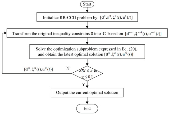
Figure 1.
The flowchart of the single-loop RB-CCD framework.
Step 1: Solve the CCD problem without considering the uncertainty of the plant design variables , and the solution values are assigned as the initial values for the RB-CCD problem.
Step 2: Transform the original inequality constraints into of Equation (18) based on . Note: starts from 1.
Step 3: Solve the optimization problem expressed in Equation (20), and obtain the latest .
Step 4: Calculate the SRI of and the values of inequality constraints ; if SRI and the values of satisfy the convergence condition in Equation (15), stop the solving process; otherwise, deliver to Step 2.
Step 5: Repeat Step 2 to Step 4 until the solution converges.
In the single-loop RB-CCD framework, the role of the random components is converting the probabilistic constraints into inequality constraints at MPP , and the role of the deterministic components is searching for the optimal plant design parameters with the inequality constraints . This means that is used to adjust the reliability-based design space of iteratively, and are located in the new reliability-based design space rather than the original feasible region. As the iterations in the RB-CCD framework proceed, the appropriate reliability-based design space is determined, and the deterministic components , as well as the control inputs , also are converged to optimal solutions and . At the same time, the main advantage of the single-loop RB-CCD framework is that it eliminates the repeated reliability analysis without increasing the number of design variables or adding equality constraints by calculating the approximate MPP of the random component via the KKT optimality conditions rather than the optimizing subproblem with the algebraic equality constraints and state equation equality constraints. Consequently, instead of performing nested design optimization and reliability loops, the single-loop RB-CCD framework solves an equivalent single-loop CCD problem, and dramatically increases the efficiency of the solution.
4. Numerical and Engineering Examples
The feasibility and effectiveness of the single-loop RB-CCD framework based on the modified RB-CCD model and SLA proposed in this work are demonstrated by two examples. The first example is a numerical case that includes two state equation equality constraints and one reliability constraint. The second example is an engineering example of the glider dynamic soaring system, which takes six state equation equality constraints, one algebraic inequality constraint, and three reliability constraints into consideration. Comparisons are made among deterministic optimization, the SORA formulation, and the single-loop RB-CCD framework. In those examples, the same convergence criterion is used, and is set as 0.001.
4.1. Example 1: A Numerical RB-CCD Example
Example 1 is a numerical RB-CCD problem containing two design variables, two state variables, and one control input; the mathematical model of this example can be described as follows:
where indicates the vector of design variables, assuming that , , , and ; means the vector of state variables, and the upper and lower bounds of are and , respectively; is control input and is limited in ; is the reliability index, and ; the initial time and final time , the initial value of is specified as when solving this RB-CCD problem by GPOPS-II [35]. In order to compare the efficiency and accuracy of the deterministic optimization for CCD, the SORA formulation and the single-loop RB-CCD framework for RB-CCD are both employed to optimize Example 1.
Firstly, the SORA formulation is utilized to decompose the modified formulation of this example into a two-level optimization structure with DO loop and RA loop. The DO loop can be formulated as
where the design variables are split into the deterministic components and the random components , and , . The state equation constraints are not only satisfied at the mean values of and , but also should be satisfied at all MPPs . , the MPPs of the random components , are calculated by the subproblem in the RA loop, and the subproblem is expressed as
where is the mapping variables of in the U-space. It is noteworthy to mention that the objective function is rather than , since the state variable is involved. The result of is a set of time series, and the inequality constraint is . Clearly, the maximum element of the set of time series is most likely to violate the inequality constraint. Hence, according to Section 3.1, is configured as the objective function to guarantee the set of time series satisfies the inequality constrain.
At the same time, the single-loop RB-CCD framework is also used to optimize this problem, and the iterative model is depicted as
where and are calculated by
where is the transformed form of the original inequality constrain , and generated by Equation (16) and Equation (17). The approximate gradient information of at point can be provided by the finite difference technique.
Table 1 compares the results of the deterministic optimization for CCD problem, the SORA formulation and the single-loop framework for RB-CCD problem of Example 1. In Table 1, the vector means the optimal design, is the value of the objective function, denotes the probability of failure, and indicates the solving time of those methods. It is worth noting that 100,000 samples are selected for the CCD and RB-CCD solutions by MCS to estimate the probability of failure for the probabilistic constraint. It is clear that the of the deterministic optimization solution is 31.90%, and the drops to 0.86% with the assistance of the SORA formulation and the single-loop framework, which demonstrate that the SORA formulation and the single-loop framework for RB-CCD can effectively improve the reliability of the dynamic system compared with the deterministic optimization. The values of the objective function are increased in the SORA formulation and the single-loop framework due to the uncertainty of the design variables considered. By comparing the results of the SORA formulation and the single-loop framework for RB-CCD, it can be observed that the single-loop framework has a slight disadvantage in terms of and , but it has considerably higher solving efficiency than the SORA formulation and significantly reduces the running time.

Table 1.
The results of CCD and RB-CCD for Example 1.
In attempting to graphically display the results of the MCS for the state trajectories of the solutions of the CCD and RB-CCD methods, 1000 samples are used to create the MCS plots in Figure 2, Figure 3 and Figure 4. Obviously, in Figure 2, a large number of trajectories of violate the inequality constraint, while only a small number of ones in Figure 3 and Figure 4 violate the inequality constraint. Meanwhile, the optimal control curves for the CCD and RB-CCD solutions are also plotted in Figure 5.
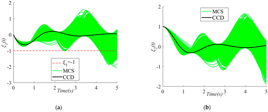
Figure 2.
MCS plots of state variables in the solution of CCD: (a) , (b) .
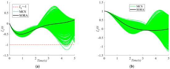
Figure 3.
MCS plots of state variables in the solution of SORA: (a) , (b) .
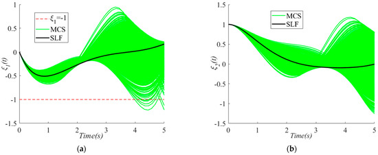
Figure 4.
MCS plots of state variables in the solution of SLF: (a) , (b) .
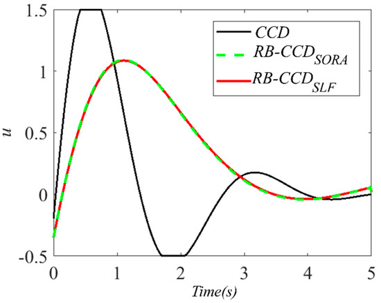
Figure 5.
The optimal control curves in CCD and RB-CCD.
4.2. Example 2: The RB-CCD Problem for the Glider Dynamic Soaring System
Dynamic soaring is the art of unpowered flight by exploiting wind gradients at high altitude. The glider dynamic soaring system is a multidisciplinary dynamic system involving physical design, aerodynamics, and control engineering. It is a classical complicated problem and has been extensively studied in a deterministic manner [36,37]. However, the uncertainty stemming from the stochastic design variables might have a negative influence on the performance of the glider dynamic soaring system. Thus, the RB-CCD problem for the glider dynamic soaring system deserves further study to improve the reliability of the glider dynamic soaring system.
In this work, the least-required wind gradient slope that can sustain an energy-neutral dynamic soaring flight is optimized in the deterministic and uncertain manners; i.e., the CCD problem and the RB-CCD problem of the glider soaring system are solved. In the control co-design of the glider soaring system, a point-mass model is adequate for reflecting the motion characteristics of the glider. Three-dimensional point-mass equations of motion for a generic glider can be derived as follows:
where and are computed by the following expression:
In the above, is the glider mass, denotes the (East, North) position, is the altitude, and stands for the airspeed. means the air-relative flight path angle, is the heading angle measured clockwise from the North, and means the glider bank angle. and are the wind component along the East direction and the time rate of change in the wind component, and is the average wind gradient slope. and are the lift force and drag force, respectively.
where is the lift coefficient, is the drag coefficient, is the parasitic drag coefficient, denotes the induced drag factor. means area of the trapezoidal wing calculated by the bases and the height , which are showed in Figure 6.
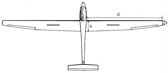
Figure 6.
The sketch of the glider: and are the bases, is the height of the trapezoidal wing.
4.2.1. The CCD Problem for the Glider Dynamic Soaring System
The objective of the CCD problem for the glider dynamic soaring system is to determine the least required slope of a linear wind gradient profile that can still sustain a powerless dynamic soaring flight, that is,
subject to the state equations in Equation (26) and the following constraints:
and the following boundary conditions:
where are design variables, the vector means the state variables, and is chosen as the vector of control inputs. The lower and upper bounds on the design parameters are and , The box bounds of the state variables and , the control inputs are limited by and , and . The maximum allowable area , the maximum aspect ratio , and the minimum allowable value for maximum height .
GPOPS-II is applied to solve the above CCD problem of the glider dynamic soaring system, the optimal values of the objective function and design variables are listed in Table 2, and the optimal state trajectories and control curves are exhibited in Figure 7 and Figure 8.
Table 2.
The results of CCD and RB-CCD for the glider dynamic soaring system.
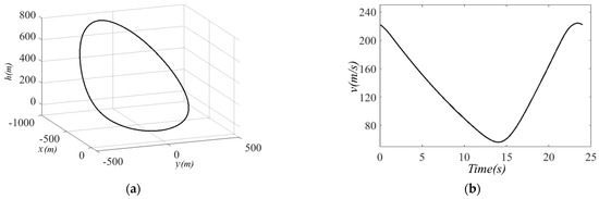
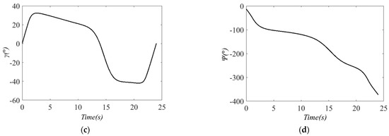
Figure 7.
The optimal state trajectories in CCD of the glider dynamic soaring system: (a) , (b) , (c) , (d) .
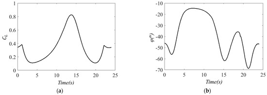
Figure 8.
The optimal control curves in CCD of the glider dynamic soaring system: (a) , (b) .
4.2.2. The RB-CCD Problem for the Glider Dynamic Soaring System
Differently from CCD, RB-CCD for the glider dynamic soaring system takes into account the uncertainty of the plant design variables , and assuming that the standard deviations of are , , and . More importantly, the RB-CCD problem for the glider dynamic soaring system subjects to the following reliability constraints given in Equation (32) rather than inequality constraints given in Equation (30):
To solve the above RB-CCD problem, the SORA method, and the single-loop framework based on the modified RB-CCD model and SLA proposed in this work, are employed. The subproblems of DO loop and RA loop in the SORA method to optimize this problem are expressed as follows:
where the plant design variables are split into the deterministic components and the random components , and . The state equation constraints are not only satisfied at the mean values of and , but also need to be met at all MPPs . Additionally, is obtained in the RA process of the previous cycle, the subproblem in the RA loop can be expressed as
where are known and delivered from the RA process of the previous cycle, are the mapping variables of in U-space.
Instead of solving the subproblem given in Equation (34), the single-loop framework adopts an approximate formula to search the MPP . Hence, can be calculated by
The results of the RB-CCD problem for the glider dynamic soaring system solved by the SORA method and the single-loop framework are also compared in Table 2. The physical design vector has been modified on average by 7.51% compared to the deterministic situation, while the objective value has changed by only 0.31% due to the control inputs, which have also adjusted accordingly to achieve the optimal objective value. Comparing the results of RB-CCD optimized by the SORA method and the single-loop framework, it is clear that the single-loop framework can provide a solution with the same accuracy as the SORA method while consuming less time.
At the same time, the probabilities of failure () for all performance measure functions in Equation (32) are benchmarked MCS with n = 100,000 samples, as listed in Table 3, it is quite apparent that the of the reliability constraints and , at 1.25% and 25.78%, drop 0.18% and 0.20% (and 0.38%), respectively, with the assistance of the SORA method and the single-loop framework, which demonstrates that the SORA method and the single-loop framework for RB-CCD can effectively improve the reliability of the glider dynamic system. According to Table 2 and Table 3, it is clear that the single-loop framework, the proposed approximate solving framework, significantly improves the solving efficiency with retaining the accuracy of the solution compared to SORA in the glider dynamic soaring system.
Table 3.
Probabilities of failure using MCS with n = 100,000 samples.
To intuitively demonstrate the optimal state trajectories and control curves of the RB-CCD problem for the glider dynamic soaring system solved by the SORA method and the single-loop framework, Figure 9 shows the trajectories of all state variables, and Figure 10 exhibits the curves of all control inputs. Finally, 1000 samples are used to create the MCS plots in Figure 11 to illustrate the MCS of the state trajectories in the solution of the single-loop framework. It can be observed that under uncertainty, states trajectories yielded by MCS of the system tend to deviate from the optimal states trajectories.
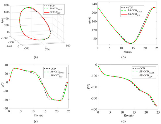
Figure 9.
The optimal state trajectories in RB-CCD optimized by SORA and SLF: (a) , (b) , (c) , (d) .
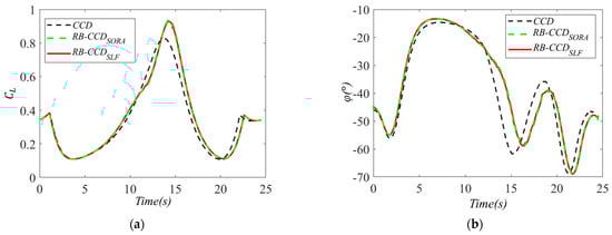
Figure 10.
The optimal control curves in RB-CCD optimized by SORA and SLF: (a) , (b) .
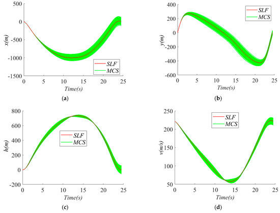
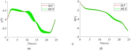
Figure 11.
MCS plots of state variables in the solution of the single-loop framework: (a) , (b) , (c) , (d) , (e) , (f) .
5. Conclusions
In attempting to eliminate the undesirable effect of the uncertainty stemming from the stochastic design variables on the performance of the dynamic system, this work investigates the RB-CCD problem. Firstly, the modified model for RB-CCD is deduced by introducing additional design variables and constraints (state equations and algebraic equality constraints) to transform the probabilistic constraint with state variables into inequality constraints. Then, a single-loop framework based on the modified RB-CCD model and SLA is proposed to enhance the efficiency of solving the RB-CCD problem by transforming the modified RB-CCD model into an equivalent single-loop deterministic CCD model. Theoretically, the presented single-loop framework performs better than the SORA method with respect to efficiency, since it adopts reliability information from the approximate method rather than the complex optimization subproblem. Finally, a numerical case and an engineering case validate the accuracy and efficiency of the single-loop framework in practice.
The contributions of this work mainly include the following:
- (a)
- It deduces the modified RB-CCD model to transform the probabilistic constraint into inequality constraints, and lays a cornerstone for solving the RB-CCD problem in which the probabilistic constraint contains plant design parameters, state variables, and control inputs.
- (b)
- It proposes a single-loop RB-CCD framework based on the modified model and SLA, which can convert the RB-CCD problem into an equivalent single-loop deterministic CCD problem to facilitate the optimization of RB-CCD.
- (c)
- It solves the RB-CCD problem in the glider dynamic soaring system with high efficiency, and significantly improves the reliability of the glider dynamic soaring system.
However, considering the effect of uncertainty stemming from the control input on the system is also a challenging task, due to the fact that the control input is the time-dependent curve rather than a fixed point. Thus, more efforts will be made in the future to perform uncertainty analysis on the control input.
Author Contributions
Methodology, Q.Z. and Y.W.; software, Q.Z. and P.Q.; writing—original draft, Q.Z.; and writing—review and editing, Y.W. and L.L. All authors have read and agreed to the published version of the manuscript.
Funding
This work was supported by the National Key Research and Development Program of China (Grant No. 2018YFB1700905) and National Natural Science Foundation of China (Grant No. 51575205).
Institutional Review Board Statement
Not applicable.
Informed Consent Statement
Not applicable.
Data Availability Statement
Researchers interested in this method can access the code through the corresponding author.
Conflicts of Interest
The authors declare no potential conflict of interest.
References
- Allison, J.T.; Herber, D.R. Multidisciplinary design optimization of dynamic engineering systems. AIAA J. 2014, 52, 691–710. [Google Scholar] [CrossRef]
- Zhang, Q.; Wu, Y.; Lu, L. A Novel Surrogate Model-Based Solving Framework for the Black-Box Dynamic Co-Design and Optimization Problem in the Dynamic System. Mathematics 2022, 10, 3239. [Google Scholar] [CrossRef]
- Herber, D.R.; Allison, J.T. Nested and Simultaneous Solution Strategies for General Combined Plant and Control Design Problems. J. Mech. Des. 2018, 141, 011402. [Google Scholar] [CrossRef]
- Betts, J.; Kolmanovsky, I. Practical Methods for Optimal Control using Nonlinear Programming. Appl. Mech. Rev. 2002, 55, B68. [Google Scholar] [CrossRef]
- Serrancolí, G.; Pàmies-Vilà, R. Analysis of the influence of coordinate and dynamic formulations on solving biomechanical optimal control problems. Mech. Mach. Theory 2019, 142, 103578. [Google Scholar] [CrossRef]
- García-Vallejo, D.; Font-Llagunes, J.M.; Schiehlen, W. Dynamical analysis and design of active orthoses for spinal cord injured subjects by aesthetic and energetic optimization. Nonlinear Dyn. 2015, 84, 559–581. [Google Scholar] [CrossRef]
- Allison, J.T.; Guo, T.; Han, Z. Co-Design of an Active Suspension Using Simultaneous Dynamic Optimization. J. Mech. Des. 2014, 136, 081003. [Google Scholar] [CrossRef]
- Haemers, M.; Ionescu, C.M.; Stockman, K.; Derammelaere, S. Optimal Hardware and Control Co-Design Applied to an Active Car Suspension Setup. Machines 2021, 9, 55. [Google Scholar] [CrossRef]
- Azad, S.; Behtash, M.; Houshmand, A.; Alexander-Ramos, M.J. PHEV powertrain co-design with vehicle performance considerations using MDSDO. Struct. Multidiscip. Optim. 2019, 60, 1155–1169. [Google Scholar] [CrossRef]
- Deshmukh, A.P.; Allison, J.T. Multidisciplinary dynamic optimization of horizontal axis wind turbine design. Struct. Multidiscip. Optim. 2015, 53, 15–27. [Google Scholar] [CrossRef]
- Du, X.; Chen, W. Sequential Optimization and Reliability Assessment Method for Efficient Probabilistic Design. J. Mech. Des. 2004, 126, 225–233. [Google Scholar] [CrossRef]
- Lu, L.; Wu, Y.; Zhang, Q.; Qiao, P. A Transformation-Based Improved Kriging Method for the Black Box Problem in Reliability-Based Design Optimization. Mathematics 2023, 11, 218. [Google Scholar] [CrossRef]
- Jeon, K.; Yoo, D.; Park, J.; Lee, K.D.; Lee, J.J.; Kim, C.W. Reliability-Based Robust Design Optimization for Maximizing the Output Torque of Brushless Direct Current (BLDC) Motors Considering Manufacturing Uncertainty. Machines 2022, 10, 797. [Google Scholar] [CrossRef]
- Li, X.; Zhu, H.; Chen, Z.; Ming, W.; Cao, Y.; He, W.; Ma, J. Limit state Kriging modeling for reliability-based design optimization through classification uncertainty quantification. Reliab. Eng. Syst. Saf. 2022, 224, 108539. [Google Scholar] [CrossRef]
- Li, M.; Wang, Z. Surrogate model uncertainty quantification for reliability-based design optimization. Reliab. Eng. Syst. Saf. 2019, 192, 106432. [Google Scholar] [CrossRef]
- Ghazaan, M.I.; Saadatmand, F. A new performance measure approach with an adaptive step length selection method hybridized with decoupled reliability-based design optimization. Structures 2022, 44, 977–987. [Google Scholar] [CrossRef]
- Li, F.; Liu, J.; Wen, G.; Rong, J. Extending SORA method for reliability-based design optimization using probability and convex set mixed models. Struct. Multidiscip. Optim. 2018, 59, 1163–1179. [Google Scholar] [CrossRef]
- Zhang, J.; Gao, L.; Xiao, M.; Lee, S.; Eshghi, A.T. An active learning Kriging-assisted method for reliability-based design optimization under distributional probability-box model. Struct. Multidiscip. Optim. 2020, 62, 2341–2356. [Google Scholar] [CrossRef]
- Cheng, G.; Xu, L.; Jiang, L. A sequential approximate programming strategy for reliability-based structural optimization. Comput. Struct. 2006, 84, 1353–1367. [Google Scholar] [CrossRef]
- Li, F.; Wu, T.; Hu, M.; Dong, J. An accurate penalty-based approach for reliability-based design optimization. Res. Eng. Des. 2009, 21, 87–98. [Google Scholar] [CrossRef]
- Zhang, X.; Lu, Z.; Cheng, K. Reliability index function approximation based on adaptive double-loop Kriging for reliability-based design optimization. Reliab. Eng. Syst. Saf. 2021, 216, 108020. [Google Scholar] [CrossRef]
- Chen, X.; Hasselman, T.; Neill, D. Reliability based structural design optimization for practical applications. In Proceedings of the 38th Structures, Structural Dynamics, and Materials Conference, Kissimmee, FL, USA, 7–10 April 1997. [Google Scholar] [CrossRef]
- Liang, J.; Mourelatos, Z.P.; Nikolaidis, E. A Single-Loop Approach for System Reliability-Based Design Optimization. J. Mech. Des. 2007, 129, 1215–1224. [Google Scholar] [CrossRef]
- Shan, S.; Wang, G.G. Reliable design space and complete single-loop reliability-based design optimization. Reliab. Eng. Syst. Saf. 2008, 93, 1218–1230. [Google Scholar] [CrossRef]
- Li, F.; Wu, T.; Badiru, A.; Hu, M.; Soni, S. A single-loop deterministic method for reliability-based design optimization. Eng. Optim. 2013, 45, 435–458. [Google Scholar] [CrossRef]
- Yang, M.; Zhang, D.; Jiang, C.; Han, X.; Li, Q. A hybrid adaptive Kriging-based single loop approach for complex reliability-based design optimization problems. Reliab. Eng. Syst. Saf. 2021, 215, 107736. [Google Scholar] [CrossRef]
- Hao, P.; Yang, H.; Yang, H.; Zhang, Y.; Wang, Y.; Wang, B. A sequential single-loop reliability optimization and confidence analysis method. Comput. Methods Appl. Mech. Eng. 2022, 399, 115400. [Google Scholar] [CrossRef]
- Cui, T.; Allison, J.T.; Wang, P. A Comparative Study of Formulations and Algorithms for Reliability-Based Co-Design Problems. J. Mech. Des. 2019, 142, 031104. [Google Scholar] [CrossRef]
- Azad, S.; Alexander-Ramos, M.J. A Single-Loop Reliability-Based MDSDO Formulation for Combined Design and Control Optimization of Stochastic Dynamic Systems. J. Mech. Des. 2020, 143, 021703. [Google Scholar] [CrossRef]
- Cui, T.; Allison, J.T.; Wang, P. Reliability-based control co-design of horizontal axis wind turbines. Struct. Multidiscip. Optim. 2021, 64, 3653–3679. [Google Scholar] [CrossRef]
- Ross, I.M.; Karpenko, M. A review of pseudospectral optimal control: From theory to flight. Annu. Rev. Control. 2012, 36, 182–197. [Google Scholar] [CrossRef]
- Li, M.; Peng, H. Solutions of nonlinear constrained optimal control problems using quasilinearization and variational pseudospectral methods. ISA Trans. 2016, 62, 177–192. [Google Scholar] [CrossRef] [PubMed]
- Betz, W.; Papaioannou, I.; Straub, D. Bayesian post-processing of Monte Carlo simulation in reliability analysis. Reliab. Eng. Syst. Saf. 2022, 227, 108731. [Google Scholar] [CrossRef]
- Du, X.; Huang, B. Reliability-based design optimization with equality constraints. Int. J. Numer. Methods Eng. 2007, 72, 1314–1331. [Google Scholar] [CrossRef]
- Patterson, M.A.; Rao, A.V. GPOPS-II: A MATLAB software for solving multiple-phase optimal control problems using hp-adaptive gaussian quadrature collocation methods and sparse nonlinear programming. ACM Trans. Math. Softw. 2014, 41, 1–37. [Google Scholar] [CrossRef]
- Bulirsch, R.; Nerz, E.; Pesch, H.J.; Von Stryk, O. Combining direct and indirect methods in optimal control: Range maximization of a hang glider. In Optimal Control; Bulirsch, R., Miele, A., Stoer, J., Well, K.H., Eds.; Volume 111 of International Series of Numerical Mathematics; Birkhäuser: Basel, Switzerland, 1993; pp. 273–288. [Google Scholar] [CrossRef]
- Zhao, Y.J. Optimal patterns of glider dynamic soaring. Optim. Control. Appl. Methods 2004, 25, 67–89. [Google Scholar] [CrossRef]
Disclaimer/Publisher’s Note: The statements, opinions and data contained in all publications are solely those of the individual author(s) and contributor(s) and not of MDPI and/or the editor(s). MDPI and/or the editor(s) disclaim responsibility for any injury to people or property resulting from any ideas, methods, instructions or products referred to in the content. |
© 2023 by the authors. Licensee MDPI, Basel, Switzerland. This article is an open access article distributed under the terms and conditions of the Creative Commons Attribution (CC BY) license (https://creativecommons.org/licenses/by/4.0/).