Article

PR-Alignment: Multidimensional Adaptive Registration Algorithm Based on Practical Application Scenarios

by
Wenxin Wang
1,2,*,†,‡,
Changming Zhao
1,2,†,‡ and
Haiyang Zhang
1,2,†
1
Key Laboratory of Photoelectronic Imaging Technology and System, Ministry of Education, Beijing 100081, China
2
Key Laboratory of Photonics Information Technology, Ministry of Industry and Information Technology, Beijing 100081, China
*
Author to whom correspondence should be addressed.
Current address: School of Optics and Photonics, Beijing Institute of Technology, Beijing 100081, China.
These authors contributed equally to this work.
Machines 2023, 11(2), 254; https://doi.org/10.3390/machines11020254
Submission received: 16 January 2023 / Revised: 7 February 2023 / Accepted: 7 February 2023 / Published: 8 February 2023
(This article belongs to the Section Robotics, Mechatronics and Intelligent Machines)

Abstract

:
In the present day, 3D point clouds are considered to be an important form of representing the 3D world. In computer vision, mobile robotics, and computer graphics, point cloud registration is a basic task, and it is widely used in 3D reconstruction, reverse engineering, among other applications. However, the mainstream method of point cloud registration is subject to the problems of a long registration time as well as a poor modeling effect, and these two factors cannot be balanced. To address this issue, we propose an adaptive registration mechanism based on a multi-dimensional analysis of practical application scenarios. Through the use of laser point clouds and RGB images, we are able to obtain geometric and photometric information, thus improving the data dimension. By adding target scene classification information to the RANSAC algorithm, combined with geometric matching and photometric matching, we are able to complete the adaptive estimation of the transformation matrix. We demonstrate via extensive experiments that our method achieves a state-of-the-art performance in terms of point cloud registration accuracy and time compared with other mainstream algorithms, striking a balance between expected performance and time cost.

1. Introduction

Among the many forms in which 3D data can be represented, depth images, polygonal meshes, and point clouds can be used to represent the real physical world [1,2]. In recent years, the maturity and widespread use of 3D point cloud data acquisition equipment, such as Lidar, as well as the improvement in computing capabilities, have led to the widespread use of point cloud data [3,4,5,6]. The point cloud data collected by different stations may have some deviations due to the differing angles and frames used to collect point cloud data, as shown in Figure 1. With point cloud alignment technology, it is possible to unify different frames of point clouds under the same coordinate system, which is an effective solution to this issue [7]. As an unstructured data form with occlusion [8], noise [9,10], and large amounts of data [11,12], point cloud registration has proven to be a challenging research direction in point cloud data processing. It needs to be performed precisely and quickly in order to achieve the desired results. In this paper, the main focus is on rigid registration of point clouds, which is the registration of point clouds by translation and rotation alone, without scaling or deformation. There are many applications of point cloud registration technology, such as simultaneous localization and mapping (SLAM) for mobile robots [13,14], high-quality map construction [15], environmental awareness for autonomous vehicles [16], forest structure parameter evaluation, city modeling, augmented reality (AR) scene detection, image synthesis for medical detection, construction monitoring, and as-built modeling, among others [17,18]. Alignment accuracy is often required in these application scenarios, as well as very fast alignment speeds in some cases.
The performance of these applications can be greatly enhanced by highly accurate and fast alignment algorithms. Currently, point cloud registration methods are categorized as either traditional non-learning alignment methods [19,20] or deep learning-based alignment methods [21,22,23]. The non-learning registration method, however, was found to have many problems during the implementation of the registration scheme, including an easy fall into local minima, poor generalization, time consumption, and the use of manual features for separating correspondences during the implementation phase. Moreover, the actual registration effect may be influenced by the designer’s experience and ability to adjust the parameters. There has been significant progress in deep learning in recent years, and more and more algorithms have improved their performance through deep learning, which has been widely applied to point cloud registration [24,25]. Speed improvements have been achieved by a large number of algorithms, and they have been shown to be robust to noise, low overlap, and occlusions. In the field of point cloud registration, learning-based methods have the potential to improve performance. While the deep learning method represented by PointNet improves the processing speed and robustness of the algorithm to a certain degree, it is often less mature than the non-learning method and is still primarily focused on simple object alignment. Furthermore, a number of issues also need to be considered, including the need for more computational resources, the difficulty of implementing it, the difficulty of interpreting it, and the need for extensive training.
Based on practical application requirements, this paper selects a more mature and easy-to-deploy non-learning approach as the research object. To overcome many of the problems associated with traditional methods, we propose an adaptive registration algorithm, PR-Alignment, that takes into account the actual application environment. By introducing laser point clouds and RGB image information, this method increases the dimensionality of the data. We use the NARF and FPFH methods to detect and describe 3D feature points in laser point clouds, establish a matching relationship between feature point pickup and local feature description, and create the geometric matching point set M g by ranking the matching points from strong to weak. For RGB images, the SIFT algorithm is used to detect and describe the two-dimensional feature points and to complete the matching between the source and target frames. Following this, the two-dimensional matching relationship is mapped to the three-dimensional space using bilinear interpolation. Based on the ranking of the matches from strong to weak, the photometric matching point set M p is generated. A mixed matching point set M c is generated by combining the environmental information by fusing M g and M p , and then a robust and effective estimation of the transformation matrix is achieved by combining a biased random sampling method and an adaptive evaluation criterion. Lastly, the registration process of 3D point clouds is completed by combining ICP. Through extensive validation experiments on the Semantic 3D dataset and our own collected dataset, we found that our proposed algorithm has significantly improved speed and accuracy.
Briefly, our contributions include:
  • Data collection of the scene point cloud is carried out by using the UAV-borne Lidar system, and the point cloud is then preprocessed before being used for analysis. The structure composition and working principle of the point cloud data acquisition system was studied, a calibration experiment for the point cloud data acquisition system was designed and completed, and the internal parameters and relative positional relationship between the color camera and laser radar were determined. An experiment to acquire 3D point clouds of the scene has been completed, and a colored point cloud has been produced. Moreover, for the pre-processing of scene point cloud, the efficient organization of point cloud data is realized based on the data structure of a K–D tree, and an adaptive voxel grid down-sampling method is proposed to ensure a good and stable down-sampling effect. The unreliable outliers are eliminated by statistical filtering, and the point cloud normal vector is estimated based on PCA.
  • An algorithm for coarse registration of point clouds based on improved RANSAC is studied. We use NARF and FPFH to detect, describe, and match 3D key points on 3D point clouds, along with the establishment of geometric homonym point pairs. For color images, SIFT is used to detect, describe, and match two-dimensional key points, and their values are obtained through bilinear interpolation, resulting in the establishment of photometric point pairs with the same name. Geometric matching and photometric matching are combined adaptively according to the judgment of the current scene category. Aiming at the deficiency of the traditional RANSAC algorithm, an improved RANSAC algorithm is proposed innovatively, which sets the bias of random sampling and establishes an adaptive hypothesis evaluation method, which shows that the validity and robustness of transformation matrix estimation are improved.
  • A scene classification algorithm is studied. A binary validity template is proposed to filter out invalid information from the local description of the luminosity texture features and geometric structure features of the scene by using the LBP and CLBP operators, and the scene feature vector is extracted by computing the normalized statistical histogram of the LBP and CLBP operators. For scene classification, a three-class SVM is used, and the labeled dataset is constructed by using a combination of self-built point cloud data and third-party data.

2. Related Work

In the course of this paper, there are three components that are worth noting: ICP-variants, point-set alignment, and feature point matching.
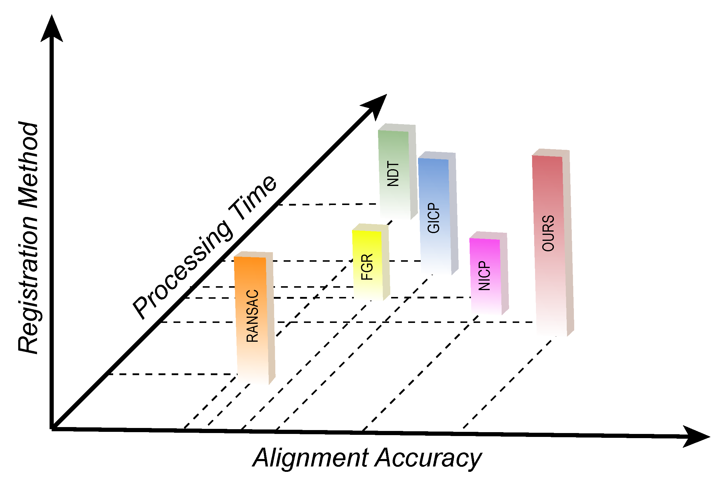
ICP-variants. The iterative closest point (ICP) is one of the most classical algorithms for registering point clouds. It estimates the transformation matrix by iteratively searching for corresponding points and minimizing their overall distance [26,27,28,29]. As a result of calculating the Euclidean distance between two point clouds, the algorithm determines the corresponding points between them, constructs a rotation and translation matrix based on these points, estimates the error function between the transformed source and target point clouds, and iterates until the error is less than the set threshold. As a result of iterative calculation, the ICP algorithm has relatively good accuracy, but it is relatively slow because of its iterative nature [30,31]. The algorithm is highly dependent on the initial positions of the two point clouds, and it may result in a local optimum for the objective function. Several variants based on the ICP algorithm have been developed in order to address this problem [32,33,34]. The GICP introduces probabilistic information (in the form of a covariance array) and proposes a model of ICP that addresses both point-to-point and point-to-surface ICP, as well as surface-to-surface ICP [35,36]. In addition to constraints on the distance between points, NICP adds constraints on the normal vector and curvature of the surface on which the point cloud is located [37,38]. A comparison of the registration effects between the different methods is shown in Figure 2. In this paper, we present an improved RANSAC in which the sampling bias for geometric matching and photometric matching can be adjusted depending on the environment and in which adaptive evaluation criteria can be applied to the evaluation process.
Point-set alignment. For the alignment of 3D point clouds, several methods are available. ICP, NDT algorithms, and their variants require that the point clouds are already roughly aligned or have a priori poses such as IMU, GNSS, odometry, etc. Otherwise, coarse alignment is required to provide an initial pose for them. In the subsequent work, much attention will be devoted to finding more robust correspondence, such as point-to-point, face-to-face, and feature-to-feature correspondence [39,40]. By utilizing these correspondences, alignment parameters are estimated, thereby improving the accuracy of point cloud alignment and reducing the reliance on the correct initial poses. Another method of coarse alignment is based on the allometric four-point-cloud set (4PCS) under rigid transformation, where the transformation of some points is also the transformation of all points, and the most accurate transformation is obtained by verifying multiple sets of allometric sets. There are, however, several problems associated with these alignment methods, including poor alignment, long alignment times, and manual settings. The use of additional ground real gestures may facilitate the learning of geometric characteristics from point clouds in some learning methods [41,42,43]. The process of collecting these basic and accurate annotations, however, is not straightforward. In recent years, unsupervised learning methods have been developed, such as UR & R [44] and BYOC [45], which strengthen the training of cross-view geometry and visual consistency before hidden supervision registration takes place. However, the features used for correspondence extraction are either directly based on RGB data or are trained by pseudo-correspondence tags in visual correspondence, where visual and geometric cues are usually extracted independently without effective use of their correlations. Moreover, the coarse-matching algorithm for point clouds based on local attributes includes the detection, description, and matching of key points as well as an estimation of the transformation matrix based on random sampling consistency (RANSAC). Generally, it is feasible to combine three-dimensional geometric characteristics with two-dimensional light characteristics, using RANSAC to generate the point clouds across continuous frames based on the richness of both types of information [46,47]. It is noteworthy, however, that traditional RANSAC cannot be applied to the matching relationship between combining different methods due to an unbalanced base of geometric matching and optical matching, thus ensuring that the transformation matrix estimation is stable and effective. Consequently, this problem will become even more acute as the overlapping area decreases. Based on the environment characteristics, we establish geometric and photometric matching point pair sets, which can optimize the alignment effect and enable adaptive parameter adjustment at the same time.
Feature point matching. The use of features for matching is an important method for achieving coarse point cloud registration. The point feature histogram (PFH), developed by Rusu et al.  [48], estimates surface conditions using the normal vector between neighboring point clouds and point cloud features [49,50,51]. As a result of the improved fast point feature histogram (FPFH), the computation time for feature points has been further reduced [52,53]. Guo et al. proposed a three-dimensional shape context (3DSC) [54,55]. A vector value is used to establish a correspondence between different surface points, and its shape characteristics are described based on the value of the vector. In this paper, we use NARF [56,57], FPFH, SIFT, and bilinear interpolation methods for key point detection and description.

3. Methodology

3.1. Overview

Our proposed adaptive registration algorithm is based on practical application scenarios in order to address the problems associated with traditional registration methods, such as poor results and long registration times. We introduce the principle of 3D point cloud alignment by combining theory with pictures to demonstrate that the most important part of this paper is the solution of the optimal transformation matrix T (Section 3.2).
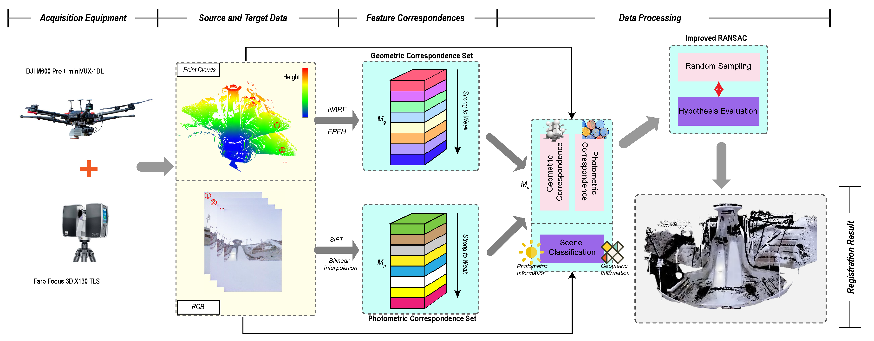
After point cloud data and RGB images have been extracted, geometric matching point pair sets M g , photometric matching point pair sets M p , and mixed matching point pair sets M c are generated (Section 3.3.1). Then, we classify the scene according to the characteristics of RGB image and point clouds (Section 3.3.2). An adaptive evaluation criterion and a biased random sampling method are then used to obtain an efficient and robust estimation of the transformation matrix (Section 3.3.3). The full pipeline is illustrated in Figure 3.

3.2. 3D Registration Model

As part of the registration, point clouds from different perspectives obtained are merged into the same three-dimensional coordinate system in order to obtain a complete geometric model [58,59,60,61], as shown in Figure 4. It is possible to represent the rigid transformation of the model in the space coordinate system using a rotation–translation matrix, referred to as T in this paper. For the dynamic point cloud P = p i , i = 1 , 2 , , N p and the static point cloud Q = q j , j = 1 , 2 , , N q to be registered, the optimal Euclidean transformation matrix T must be obtained between the two point clouds in order to make the corresponding points of the overlapping parts of the two point clouds completely coincide in the spatial coordinate system. There are six undetermined parameters in the transformation matrix, namely, the translation amounts T x , T y , T z along the three coordinate axes and the rotation angles α , β , γ around the three coordinate axes. The transformation matrix T can be expressed as follows without taking into account the size of the model:
T = R X R Y R Z S
For Equation
R X = 1 0 0 0 0 cos α sin α 0 0 sin α cos α 1 0 1 0 1
R Y = cos β 0 sin β 0 0 1 0 0 sin β 0 cos β 0 0 0 0 1
R Z = cos γ sin γ 0 0 sin γ cos γ 0 0 0 0 1 0 0 1 0 1
S = 1 0 0 0 0 1 0 0 0 0 1 0 T X T Y T Z 1
In an ideal situation, the distance between the point T p i obtained by transforming a point p i in P and its corresponding point q j in Q should be 0. As a matter of fact, their distance can be expressed as follows:
d i = T P i Q j 2 .
Nevertheless, because of measurement errors and noise, the distance between corresponding points cannot reach the ideal value of 0, so the registration problem is transformed into an optimization problem, namely, finding the optimal transformation matrix to minimize the Euclidean distance between T p i and q j :
E i ( T ) = min T T P i Q j .
In conjunction with the adaptive registration algorithm proposed in this paper, the optimal transformation matrix T is subsequently determined.

3.3. Adaptive 3D Registration for PR-Alignment

3.3.1. Feature Correspondences

Using a UAV-borne Lidar or TLS scanning systems, the object can be scanned with high-density 3D point clouds and color RGB images. For the pass-through filtering of point clouds, a reliable depth range should be selected. It is critical to detect and describe 3D key points using normal aligned radial features (NARF) and FPFH, establish the matching relationships between key points in accordance with the local feature description, and sort from strong to weak based on the geometric matching point pair set M g ’s geometric matching. RGB images represent the photometric texture information of the scene, while SIFT is used to detect and describe the two-dimensional key points and to match the RGB images of the source frame and the target frame. By means of bilinear interpolation, 3D information is obtained from key points, and the 2D matching relationship is translated into 3D space. Based on the matching relationship, the photometric matching point pair set M p is sorted from strong to weak, as shown in Figure 5.
In some instances, the geometric information and the photometric information of the scene are not balanced or rich. According to the relative richness of the two types of information, this experiment categorizes the scenes into three categories: scenes with richer photometric information, marked as −1; scenes with relatively balanced geometric information and photometric information, marked as 0; scenes with richer geometric information, marked as +1. Depending on the current scene category, the geometric matching point pair set M g and the photometric matching point pair set M p are combined differently. The combined mixed-matching point pair set M c can be expressed as follows:
M c = M cg + M cp = ceiling α M g + ceiling ( 1 α ) M p
In Equation (8): | · | is the base of the set; ceiling (·) is an up-integer function; M cg and M cp are subsets of geometric and photometric matching points in M c , respectively; and α is the combination coefficient corresponding to different scene categories. Based on Equation (8), the first matching point pairs of ceiling α M g of M g and ceiling ( 1 α ) M p of M p are selected to be merged into M c . Their respective values are 0.2, 0.5, and 0.8 when the scene category is −1, 0, and +1, as suggested by the literature [47,62]. It is recommended to select fewer geometric matches and more photometric matches in a sequence when facing a scene that contains richer photometric information; in situations where geometric information and photometric information are relatively equal, select geometric matching first followed by photometric matching; whenever a scene contains richer geometric information, more geometric matches are selected sequentially over fewer photometric matches. In particular, α = 0 and α = 1 represent two edge cases where M c can only be formed with full photometric or geometric matching.
As the object environment is often cluttered, occluding, repetitive, etc., and there is a certain non-overlapping area between keyframes, many false matches are encountered. In the event of mismatching in the transformation matrix, the RANSAC algorithm must be used in order to eliminate the mismatch and make an accurate estimation of the matrix. A traditional RANSAC algorithm is employed in the literature [63,64,65,66]. For each iteration, a number of matching point pairs are randomly sampled and used to solve the transformation matrix assumption T h and calculate the interior point number p h and interior point error e h . T h is considered to be an optimal candidate if p h is greater than p th , which is the threshold for a reasonable assumption of the transformation matrix. As soon as the iteration ends, the optimal candidate with the smallest e h is selected as the output of the estimation of the transformation matrix.
The M c subset is formed by merging the M g and M p subsets. The bases of M g and M g are mainly determined by the number of key points detected. Since NARF and SIFT have different algorithmic design and application objects, M g is often much smaller than M p . Therefore, for  M c in the random sampling stage, regardless of the scene category, geometric matching is always less likely to be obtained than photometric matching. In other words, when solving T h , the participation of the two matching types is not well adapted to differing classification results. In addition, since M g is much smaller than M p , M c will have a large difference when α takes different values. In order to take into account M c under a different α , it is necessary to set p th to a smaller value according to the situation of α = 0.8. But when α = 0.2 or α = 0.5, due to the significant increase in M c , a reasonable transformation matrix assumption needs the support of more interior points. Thus, the preset smaller p th does not guarantee the rationality of the optimal candidate, and the final transformation matrix estimation is not highly reliable. The purpose of this paper is to propose an adaptive registration algorithm based on practical application scenarios. On the basis of the original RANSAC algorithm, this method has been improved by adjusting the sampling weight for geometric and photometric matching according to the scene category, as well as by adopting an adaptive evaluation standard to achieve a robust and effective estimation of the transformation matrix.

3.3.2. Scene Classification

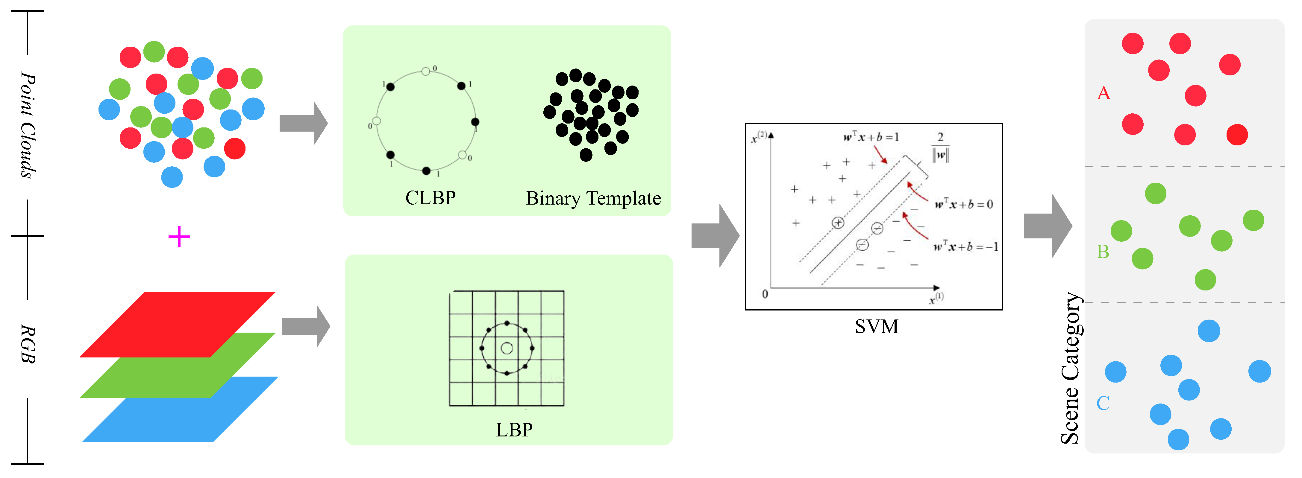
As shown in Figure 6, the flow of the algorithm for scene classification is illustrated. To extract the feature quantity of the current scene, a valid template is combined with the local binary pattern (LBP) operator and the curvature local binary pattern (CLBP) operator. The eigenvectors are input into the three-category support vector machine (SVM) to obtain the classification results.
Two-dimensional local texture features can be described using the LBP operator. It encodes the texture features of the local area by comparing the value of the central pixel of the grayscale image with its neighboring pixels. The improved LBP 8.1 ( riu 2 ) (the number of sampling points is 8, and the sampling radius is 1 pixel) is encoded in a uniform mode, which is invariant to rotation, descriptive, efficient, and robust. By taking g c as the value of the central pixel and g i ( i = 0 , , 7 ) as the value of neighboring pixels, the coded value v of LBP 8.1 ( riu 2 ) can be expressed as follows:
v = i = 0 7 s g i g c , if u 2 9 , otherwise
u = s g 7 g c s g 0 g c + i = 1 7 s g i g c s g i 1 g c
s ( x ) = 1 , x 0 0 , x < 0
In essence, CLBP approximates the local surface curvature using a second order differential to describe three-dimensional local structural features. The only difference between CLBP and LBP is that CLBP is a gradient magnitude map applied to the point cloud image. Consequently, CLBP 8.1 ( riv 2 ) can be obtained easily from LBP 8.1 ( riu 2 ) .
The scene classification algorithm uses LBP and CLBP to extract scene feature vectors. In the following description, only LBP and CLBP are referenced. In order to obtain the LBP image from the RGB image, the grayscale image must be converted, and each pixel must be encoded with LBP; the gradient magnitude image of the point cloud image is obtained using the Sobel operator, and the CLBP image is obtained by encoding each pixel with CLBP. As pixels in the dataset that are invalid or beyond the reliable depth range are considered unavailable, it is necessary to filter the LBP and CLBP images. This study constructs a binary validity template: first, the original template S i n i t with the same size as the point cloud image is established. The  S i n i t ( x , y ) value should be 0 if the pixel point ( x , y ) of the point cloud image is not available, otherwise S i n i t ( x , y ) should be 1. Since the calculation of LBP and CLBP is related to the neighboring pixels and CLBP acts on the gradient magnitude map of the point cloud image, S i n i t is corroded with a 5 × 5 convolution kernel to obtain the validity template S. The pixels of the LBP and CLBP maps must be scanned to generate the LBP and CLBP statistical histograms, and the pixels with S ( x , y ) = 0 must not be counted. As a result, the statistical histograms of both LBP and CLBP are normalized and simply connected, and the resulting 20-dimensional vector is used as the scene’s feature vector. Considering that there is still a large overlap between the source frame and the target frame, only the feature vector extracted from the source frame can be used to represent the scene features.
The scenes are classified using a three-class SVM in this study. The SVM is a supervised learning algorithm that must be trained on a labeled dataset in order to be used for classification purposes. Consequently, this paper employs category labeling for several frames in the self-constructed dataset and the Semantic 3D dataset to construct a dataset for training the classifier. For the constructed dataset, feature vectors are extracted using LBP and CLBP for SVM training and testing.

3.3.3. Random Sampling and Adaptive Evaluation

The method proposed in this paper employs a biased random sampling method and an adaptive evaluation criterion for estimating the transformation matrix for the mixed-matching point pair set M c .
At the random sampling stage, a random variable X is introduced that obeys a Bernoulli distribution whose parameter is α . Whenever X = 1, randomly select a pair of geometrically matched points from M cg ; when X = 0, randomly select a photometric matching point pair from M cp . In this case, the probability of selecting a geometric match is α and the probability of selecting a photometric match is 1− α . This means that the sampling bias of the two types of matching is appropriate for the scene category: when the scene category is −1, the luminosity matching will be more involved in the calculation of the transformation matrix assumption T h ; when the scene category is 0, the luminosity matching will be more involved in the calculation of the transformation matrix assumption T h , whereas geometric matching and photometric matching take part in the calculation of T h with the same probability, while geometric matching takes part in calculation more often when the scene category is +1.
In the hypothesis evaluation stage, the internal point number p best and the internal point error e best of the current optimal transformation matrix hypothesis T best are used as references, and the upper limit ratio parameter β ub and the lower limit ratio parameter β lb are introduced to form an adaptive evaluation standard 0 β ub 1 , 0 β lb 1 . The investigation of T h is divided into three levels based on the internal point number p h and the internal point error e h of T h . As p h > 1 + β ub p best is the acceptance domain, it is considered that there are quite a few p h , and accepting T h directly is therefore the current optimal solution. The 1 β lb p best < p h 1 + β ub p best field is the confirmation field, and it is considered that there are enough p h and that T h represents a reasonable assumption regarding the transformation matrix. However, further comparison between e h and e best is required to verify whether T h represents the current optimal transformation matrix. Using p h 1 β lb p best as the rejection domain, we will think that p h is too small and reject T h directly. In accordance with experience, this study will require β ub = β lb = 0.1 . Considering the fact that p best and e best are used as reference standards, the evaluation standard becomes self-adaptive when faced with M c formed from different combinations of variables. The introduction of β ub and β lb adds the following features. The investigation of any possible T h tends to compare the number of interior points. In order to increase the number of interior points of T best , when p best is small, the scope of confirmation domain is small. The scope of the investigation of T h tends to compare the number of interior points when p best is small. The confirmation domain is broader when p best is larger, and the investigation of T h is generally a composite comparison of the number of interior points and the number of interior point errors in order to reduce the interior point error of T best as long as sufficient interior point support is provided. As a result of such characteristics, T best retained at the end of the iteration has more interior points, which is a reasonable assumption of the transformation matrix and produces a smaller error in the interior points. In addition to being universal, this evaluation criterion also applies to the boundary cases of α = 0 and α = 1.
The pseudocode for the adaptive 3D registration method for PR-Alignment can be seen in Algorithm 1, and the process of iteration should begin after the initialization has been completed. A biased random sampling is performed on M c in one iteration, from steps 3 to 12, in order to generate a random pair of point pairs M r . Steps 13 to 15 involve the use of the singular value decomposition (SVD) algorithm to solve T h determined by M r , and to determine p h and e h . The aim of steps 16 to 22 is to determine whether T h is the current optimal transformation matrix with adaptive evaluation criteria. Iterations are terminated when the number of iterations reaches the preset upper limit or when e best is small enough. The final transformation matrix estimate is calculated by recalculating the transformation matrix determined by all interior points under T best in steps 25 to 26.
Algorithm 1 The pseudocode for the adaptive 3D registration method for PR-Alignment.
Require: Input the mix-and-match point-pair set M c
Ensure: Output the rotation–translation matrix T.
1:
Initialize T best I , p best 0 , e best , it 0 ;
2:
while  i t < i t max  and  e best e th do
3:
     X B E α ;
4:
     M r ϕ ;
5:
    while  M r < 3  do
6:
        if  X = 1  then
7:
           Make a random selection from M cg of correspondences;
8:
        else
9:
           Make a random selection from M cp of correspondences;
10:
        end if
11:
        put the correspondence into M r ;
12:
    end while
13:
    calculate T h for M r ;
14:
    transform the source keypoints in M c by T h ;
15:
    traverse M c and calculate p h and e h ;
16:
    if  p h > 1 + β ub p best  then
17:
         T best T h , p best p h , e best e h
18:
    else if  1 β lb p best < p h 1 + β ub p best  then
19:
        if  e h < e best  then
20:
            T best T h , p best p h , e best e h
21:
        end if
22:
    end if
23:
     i t i t + 1 ;
24:
end while
25:
calculate T for all the inliers of T best ;
26:
return  T
In contrast to the traditional RANSAC algorithm, the adaptive 3D registration method presented in this paper considers the particular composition of M c , provides two types of matching corresponding sampling weights based on scene category, and determines the optimal transformation matrix assumption using an adaptive evaluation standard to improve the robustness and effectiveness of the transformation matrix estimation.
As a result of the above initial registration of point clouds, the target and source point clouds have roughly coincided, but there is still a certain distance error between the two. The aim of this paper is to further improve the registration accuracy of point clouds by employing an iterative optimization algorithm, ICP, based on the principle of optimal matching. In order to minimize the overall distance between the matching points of the two sets of point clouds, the rigid body transformation matrix is calculated, and the relative pose is adjusted, thereby allowing the two sets of point clouds to be continuously estimated in terms of their corresponding point sets. Whenever the registration error is less than the preset value or the number of iterations reaches the preset value, the iteration ends, and the specific principle is as follows:
  • Perform coarse registration on the source point cloud P in order to obtain a new point cloud P T that needs to be registered. For each point p i T in P T , find the point qj closest to it in the target point cloud Q as the corresponding point pair p i T , q j .
  • Estimate the correspondence between corresponding point pairs in order to calculate the rigid body transformation matrix. Using the transformation matrix, we can obtain the average distance error D between the point in the transformed point cloud P 2 T and the corresponding point in the target point cloud Q.
    P 2 T = T × P T D = 1 n i = 1 n p i 2 T q i 2
  • In order to obtain the final rigid body transformation matrix, repeat the above steps until the set error threshold D th is reached or the maximum number of iterations I th is reached.

4. Experiments

The purpose of this section is to provide additional details regarding the implementation of the experiments and the datasets used in the experiments. An overview of the sources and information about the datasets used in the experiments is presented (Section 4.1), as well as metrics for evaluating the experimental results (Section 4.2). In addition, tables and images are presented as part of the presentation and discussion of the experimental results (Section 4.3).

4.1. Datasets and Experimental Conditions

4.1.1. Datasets

  • Self-built datasets. Three-dimensional scanning was conducted at the National Ski Jumping Center and Biathlon Ski Center for the 2022 Beijing Winter Olympics using existing airborne Lidar systems and ground-based Lidar systems (as shown in Figure 7). Laser point cloud data and RGB image sets were included in the collected data. According to the characteristics of the data and the collection environment, we have organized these data into four major categories and eight subcategories, with a total data volume of 43GB. In Table 1, we present the configuration parameters of the acquisition equipment that we used.
  • Third-party datasets. Additionally, in order to verify the universality of the method proposed in this paper, we selected the third-party database Semantic 3D for algorithm verification experiments. There are eight semantic classes that cover a wide range of urban outdoor scenes, such as churches, streets, railway tracks, squares, villages, football stadiums, and castles. Approximately four billion hand-labeled points have been evaluated, and the subversions are constantly being updated.

4.1.2. Experimental Conditions

The detailed software and hardware configurations for the performed verification experiment are shown in Table 2.

4.2. Evaluation Metrics

Methods are based on measuring the mean square error (MSE), root mean square error (RMSE), and mean absolute error (MAE) between the true and predicted values. In an ideal situation, all of these error metrics should be zero if the rigid alignment is flawless. Additionally, all angles in our results are measured in degrees.

4.3. Results and Analysis

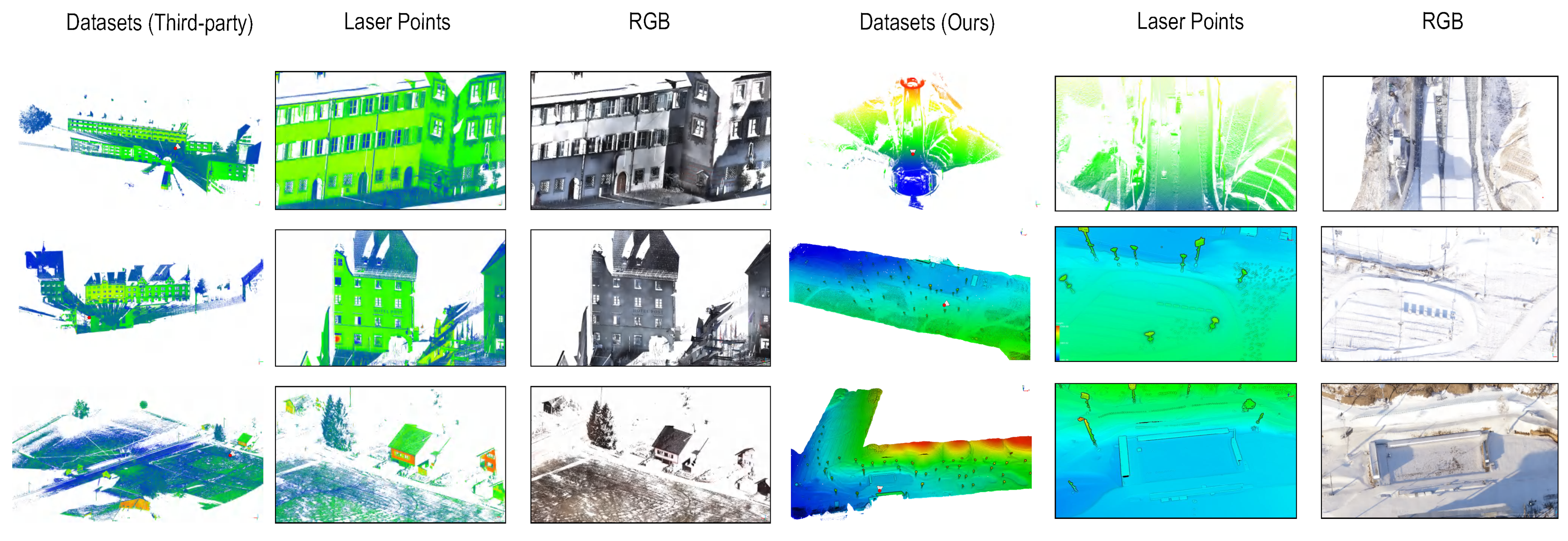
The experiment consisted of selecting three sets of data from the third-party dataset and our self-built dataset as the experimental objects. Accordingly, we selected birdfountain-station1-xyz-intensity-rgb (Bird), domfountain-station1-xyz-intensity-rgb (Dom), and sg27-station1-intensity-rgb (Sg27) from the third-party dataset. In our self-constructed dataset, we selected three-dimensional data from China’s National Ski Jumping Center (SJC), National Cross-Country Skiing Center (CSC), and National Biathlon Skiing Center (BSC). Several small samples of data from each group were selected from various perspectives as experimental objects due to the large amount of data in each group. A representation of the complete raw data, laser point cloud, and RGB information for each of the six sample sets are shown in Figure 8.
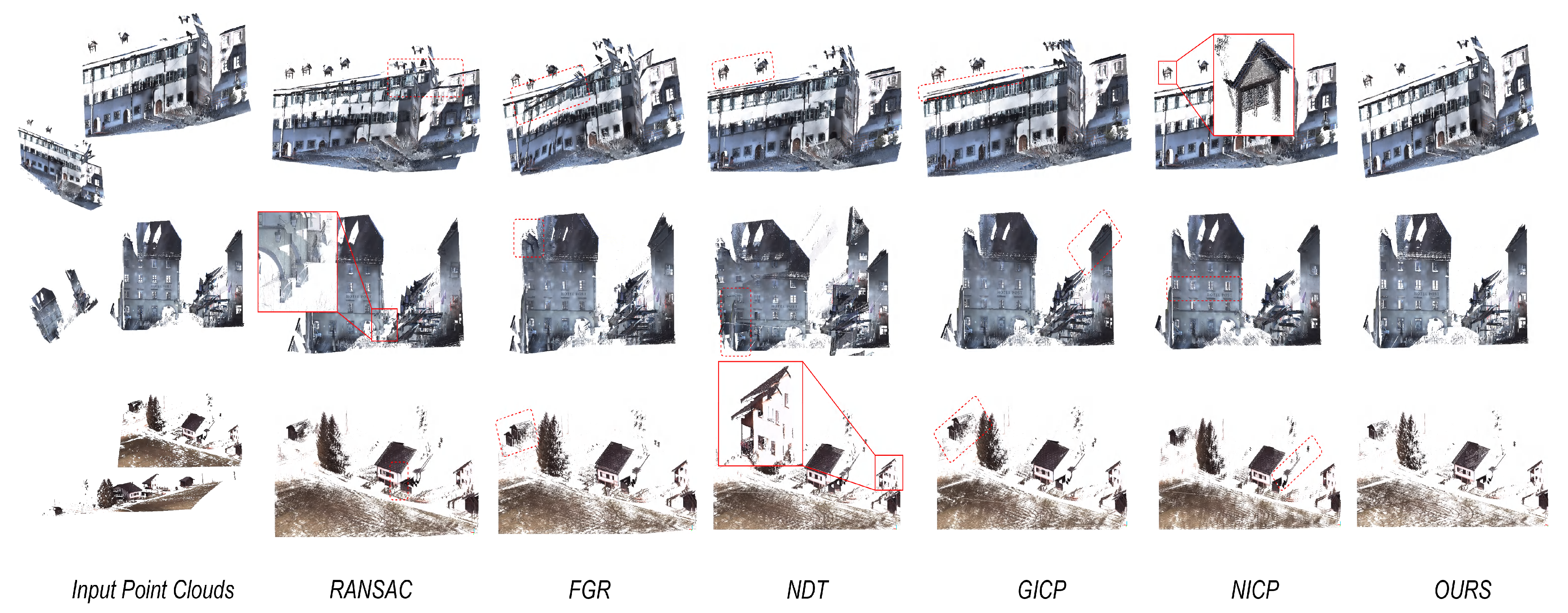
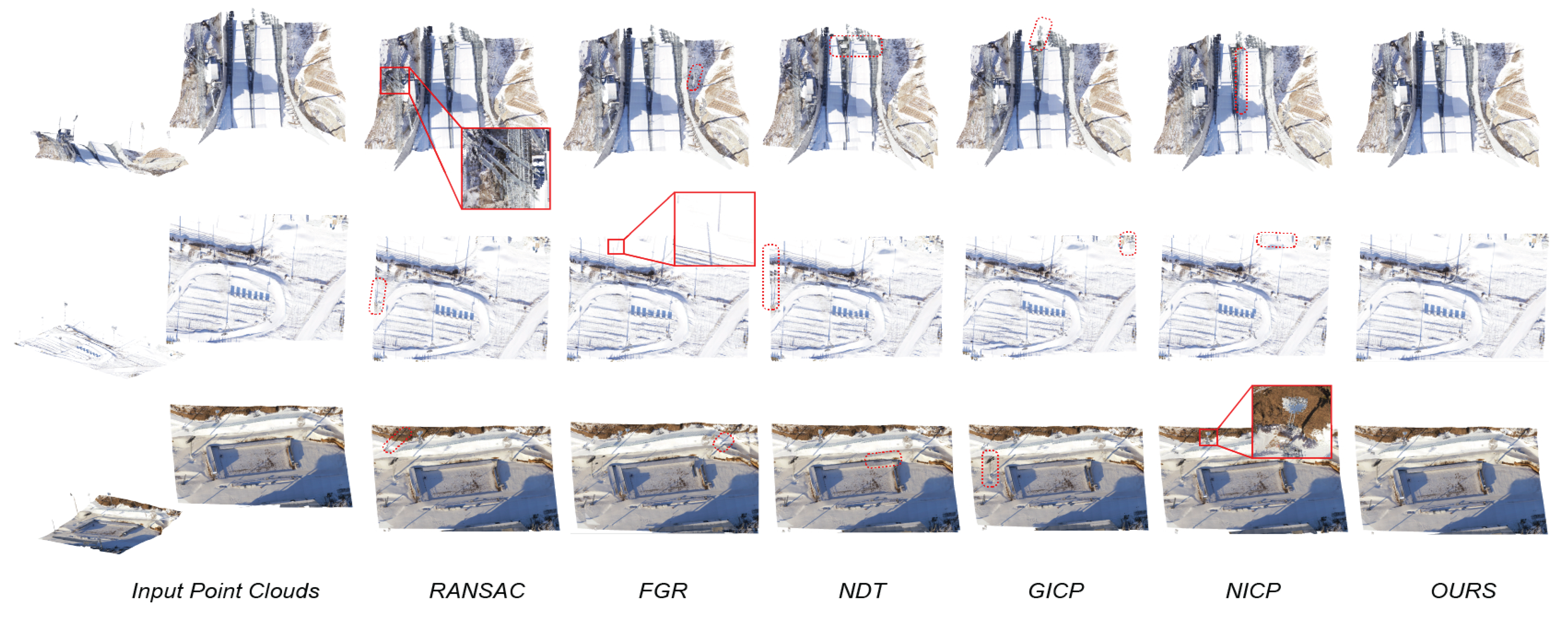
Our next step was to perform a registration test on Bird, Dom, and Sg27 in sequence in the third-party database. As part of the testing process, we used RANSAC [67], FGR [68], NDT [69], GICP [70], NICP [70], and our proposed method to test and verify the registration effect. As can be seen in Figure 9, a specific registration effect can be seen.
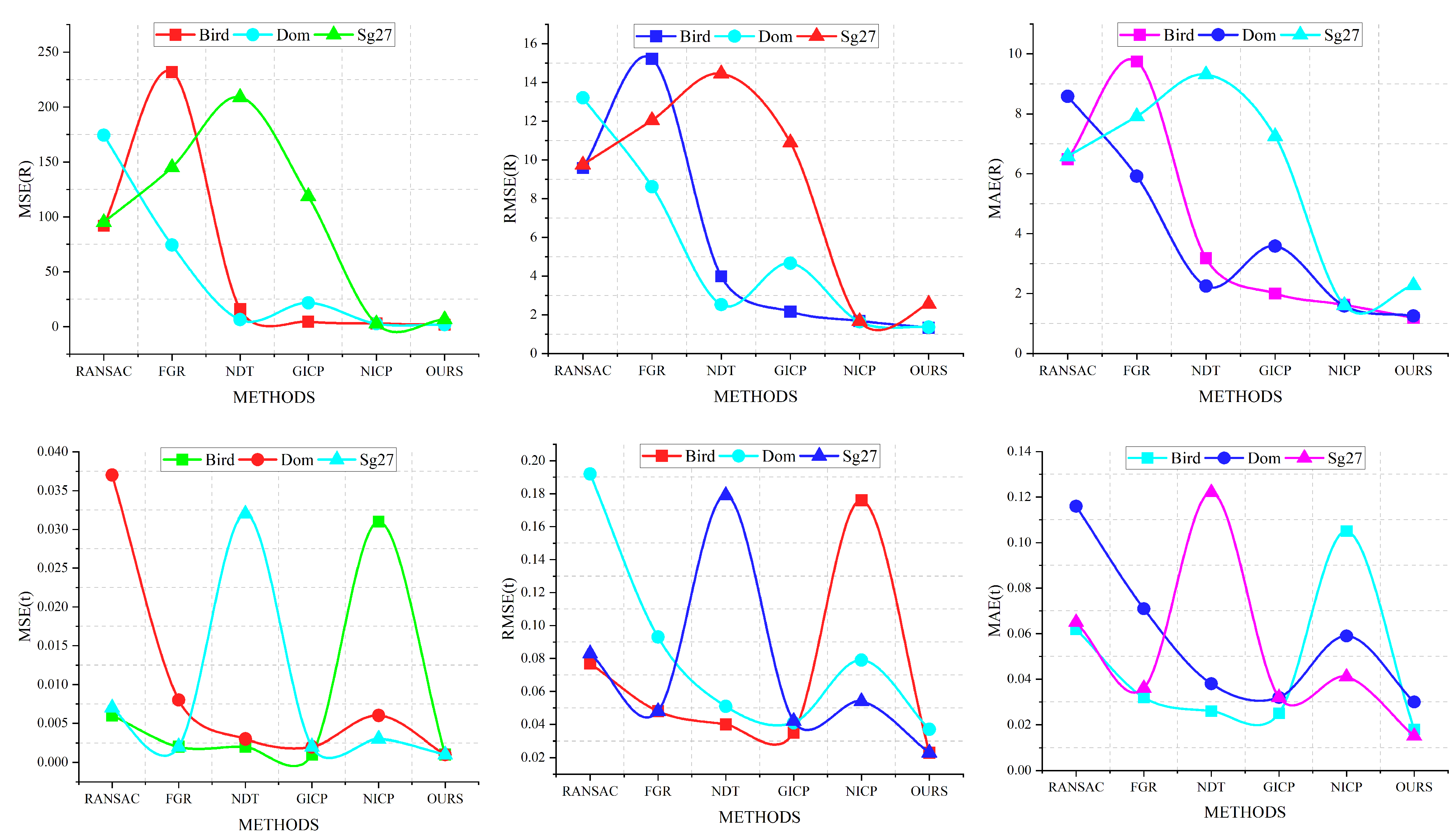
As shown in Figure 9, when using Bird data to test, FGR has the worst registration effect, followed by RANSAC, and our proposed method and NICP have excellent results. During testing with Dom data, RANSAC has the poorest registration performance, while the proposed method and NICP are still effective. Using Sg27 data, the overall registration effect is poor, and the NICP registration effect is the best, followed by the proposed method. To quantitatively assess the registration effect of each group, we use MSE, RMSE, and MAE as measurement standards, and Table 3 and Figure 10 provide evaluation results for Bird, Dom, and Sg27. We can conclude that RANSAC and FGR perform the worst, while the proposed method and NICP perform better. In light of the fact that these groups of point clouds selected as test data represent a small range of scenes, NICP demonstrates a stronger registration effect. As a result of various specific data, our method has always been able to maintain a high level of registration accuracy. According to the experimental results of this group, the method proposed in this paper has an optimal rate of 83.33% compared to other methods included in the study.
Additionally, we performed sequential registration tests on the self-built databases for SJC, CSC, and BSC. We tested and verified the registration effect using RANSAC, FGR, NDT, GICP, NICP, and our proposed method during the testing process. As shown in Figure 11, the specific registration effect is illustrated.
According to Figure 11, RANSAC performed the worst in the testing process on SJC data, while GICP and the proposed method performed relatively well. Our testing of the CSC data has shown that FGR and RANSAC have poor registration effects, while our method has the best results. As a result of testing on BSC data, the NICP algorithm performs the worst, while our method and GICP achieve good results. Together, our method achieves excellent performance when performed on SJC, CSC, and BSC datasets. The experimental results of each group were quantified and compared using quantitative statistics, as shown in Table 4 and Figure 12. As a result of our comparative analysis, we can conclude that the test results are similar to those of the third-party database. Among the six methods that participated in the test, the registration effect achieved by our proposed method was the best. The large range of scenes in these test sets of point clouds makes NICP’s registration performance unpredictable, whereas GICP is more stable. When comparing the experimental results of this group with other methods participating in the experiment, the method presented in this paper has a comprehensive optimal rate of accuracy close to 100%.
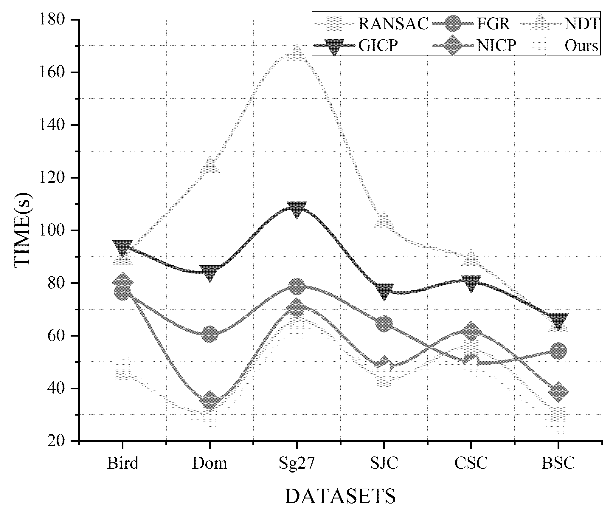
In addition to the registration effect, we also measured the effectiveness of each group of methods and calculated statistics and comparisons of the measurement results, as shown in Table 5 and Figure 13. From this, we can see that NDT and GICP have the longest processing times, which greatly reduces the efficiency of point cloud registration. RANSAC and our method have the shortest registration times. In the testing process of six groups of samples, our method takes the shortest time in 66.67% of the cases, compared to other methods.
In conclusion, compared with methods such as RANSAC, FGR, NDT, GICP, and NICP, our method balances the contradiction between registration effectiveness and processing time while maintaining good alignment performance when dealing with third-party datasets such as Bird, Dom, and Sg27, or self-built datasets such as SJC, CSC, and BSC.

5. Conclusions

Based on the type of application scenario, we propose an adaptive registration algorithm that addresses the problems of long registration times and poor modeling accuracy in the mainstream point cloud registration method. As a result of analyzing the laser point cloud, we are able to extract the geometric matching relationship of the target object, and we are also able to extract the photometric matching relationship of the target by processing the RGB image, thus increasing the dimension of the feature point data. In addition, we also added scene classification information, combined with geometric matching and photometric matching, to improve the RANSAC algorithm and complete the adaptive estimation of the transformation matrix.
We selected three samples from Semantic 3D and the self-built dataset (Bird, Dom, Sg27, SJC, CSC, BSC) for testing experiments in order to verify the effectiveness and robustness of our method. As well as comparing the accuracy of each group of algorithms in terms of MSE, RMSE, and MAE, we also compared the processing time for each group of algorithms for six samples. The results of our experiments indicate that the transformation matrix estimate calculated by our method can provide a useful initial value for the fine registration algorithm, allowing the algorithm to maintain high processing efficiency while achieving high precision.

Author Contributions

Conceptualization, W.W. and H.Z.; methodology, W.W. and C.Z.; software, W.W.; validation, W.W., C.Z. and H.Z.; formal analysis, W.W.; investigation, W.W.; resources, C.Z.; data curation, W.W.; writing—original draft preparation, W.W.; writing—review and editing, C.Z.; visualization, W.W.; supervision, C.Z. and H.Z.; project administration, C.Z.; funding acquisition, C.Z. All authors have read and agreed to the published version of the manuscript.

Funding

This research was funded by the National Key R&D Program of China, special project “Science and Technology Winter Olympics” (2018YFF0300802), and the National Natural Science Foundation of China (NSFC) (61378020, 61775018).

Data Availability Statement

Not applicable.

Acknowledgments

We thank the anonymous reviewers and members of the editorial team for their comments and contributions.

Conflicts of Interest

The authors declare no conflict of interest.

Abbreviations

The following abbreviations are used in this manuscript:
ICPIterative Closest Point
PFHPoint Feature Histogram
FPFHFast Point Feature Histogram
3DSCThree-dimensional Shape Context
T-ICPT-test-based Iterative Closest Point
ICAIndependent Component Analysis
LiDARLight Detection and Ranging
NARFNormal Aligned Radial Features
RGBRed, Green, Blue
2D and 3D2 Dimensions and 3 Dimensions
SIFTScale Invariant Feature Transform
RANSACRandom Sample Consensus
SVDSingular Value Decomposition
UAVUnmanned Aerial Vehicle
RMSERoot Mean Square Error

References

  1. Yu, J.; Zhang, C.; Wang, H.; Zhang, D.; Song, Y.; Xiang, T.; Liu, D.; Cai, W. 3d medical point transformer: Introducing convolution to attention networks for medical point cloud analysis. arXiv 2021, arXiv:2112.04863. [Google Scholar]
  2. Wang, Q.; Kim, M.K. Applications of 3D point cloud data in the construction industry: A fifteen-year review from 2004 to 2018. Adv. Eng. Inform. 2019, 39, 306–319. [Google Scholar] [CrossRef]
  3. Yang, S.; Hou, M.; Shaker, A.; Li, S. Modeling and Processing of Smart Point Clouds of Cultural Relics with Complex Geometries. ISPRS Int. J. Geo-Inf. 2021, 10, 617. [Google Scholar] [CrossRef]
  4. Zheng, S.; Zhou, Y.; Huang, R.; Zhou, L.; Xu, X.; Wang, C. A method of 3D measurement and reconstruction for cultural relics in museums. ISPRS Int. Arch. Photogramm. Remote Sens. Spat. Inf. Sci. 2012, 39, 145–149. [Google Scholar] [CrossRef]
  5. Durupt, A.; Remy, S.; Ducellier, G.; Eynard, B. From a 3D point cloud to an engineering CAD model: A knowledge-product-based approach for reverse engineering. Virtual Phys. Prototyp. 2008, 3, 51–59. [Google Scholar] [CrossRef]
  6. Urbanic, R.; ElMaraghy, H.; ElMaraghy, W. A reverse engineering methodology for rotary components from point cloud data. Int. J. Adv. Manuf. Technol. 2008, 37, 1146–1167. [Google Scholar] [CrossRef]
  7. Gupta, P.M.; Pairet, E.; Nascimento, T.; Saska, M. Landing a UAV in harsh winds and turbulent open waters. IEEE Robot. Autom. Lett. 2022, 8, 744–751. [Google Scholar] [CrossRef]
  8. Giordan, D.; Cignetti, M.; Godone, D.; Wrzesniak, A. Structure from motion multi-source application for landslide characterization and monitoring. Geophys. Res. Abstr. 2019, 21, 2364. [Google Scholar]
  9. Nguyen, T.; Pham, Q.H.; Le, T.; Pham, T.; Ho, N.; Hua, B.S. Point-set distances for learning representations of 3D point clouds. In Proceedings of the IEEE/CVF International Conference on Computer Vision, Montreal, BC, Canada, 11–17 October 2021; pp. 10478–10487. [Google Scholar]
  10. Han, X.F.; Jin, J.S.; Wang, M.J.; Jiang, W.; Gao, L.; Xiao, L. A review of algorithms for filtering the 3D point cloud. Signal Process. Image Commun. 2017, 57, 103–112. [Google Scholar] [CrossRef]
  11. Wang, W.; Zhao, C.; Zhang, H. Composite Ski-Resort Registration Method Based on Laser Point Cloud Information. Machines 2022, 10, 405. [Google Scholar] [CrossRef]
  12. Wang, W.; Zhao, C.; Zhang, H. A New Method of Ski Tracks Extraction Based on Laser Intensity Information. Appl. Sci. 2022, 12, 5678. [Google Scholar] [CrossRef]
  13. Żywanowski, K.; Banaszczyk, A.; Nowicki, M.R.; Komorowski, J. MinkLoc3D-SI: 3D LiDAR place recognition with sparse convolutions, spherical coordinates, and intensity. IEEE Robot. Autom. Lett. 2021, 7, 1079–1086. [Google Scholar] [CrossRef]
  14. Ćwian, K.; Nowicki, M.R.; Nowak, T.; Skrzypczyński, P. Planar features for accurate laser-based 3-D SLAM in urban environments. In Proceedings of the Advanced, Contemporary Control: Proceedings of KKA 2020—The 20th Polish Control Conference, Łódź, Poland, 22–25 June 2020; pp. 941–953.
  15. Musil, T.; Petrlík, M.; Saska, M. SphereMap: Dynamic Multi-Layer Graph Structure for Rapid Safety-Aware UAV Planning. IEEE Robot. Autom. Lett. 2022, 7, 11007–11014. [Google Scholar] [CrossRef]
  16. Petrlík, M.; Krajník, T.; Saska, M. LIDAR-based Stabilization, Navigation and Localization for UAVs Operating in Dark Indoor Environments. In Proceedings of the 2021 International Conference on Unmanned Aircraft Systems (ICUAS), Athens, Greece, 15–18 June 2021; pp. 243–251. [Google Scholar]
  17. Grilli, E.; Menna, F.; Remondino, F. A review of point clouds segmentation and classification algorithms. Int. Arch. Photogramm. Remote Sens. Spat. Inf. Sci. 2017, 42, 339. [Google Scholar] [CrossRef]
  18. Challis, J.H. A procedure for determining rigid body transformation parameters. J. Biomech. 1995, 28, 733–737. [Google Scholar] [CrossRef]
  19. Rusinkiewicz, S.; Levoy, M. Efficient variants of the ICP algorithm. In Proceedings of the Third International Conference on 3-D Digital Imaging and Modeling, Quebec City, QC, Canada, 28 May–1 June 2001; pp. 145–152. [Google Scholar]
  20. Olesik, J.W. Elemental analysis using icp-oes and icp/ms. Anal. Chem. 1991, 63, 12A. [Google Scholar] [CrossRef]
  21. Eggert, D.W.; Lorusso, A.; Fisher, R.B. Estimating 3-D rigid body transformations: A comparison of four major algorithms. Mach. Vis. Appl. 1997, 9, 272–290. [Google Scholar] [CrossRef]
  22. Livieratos, L.; Stegger, L.; Bloomfield, P.; Schafers, K.; Bailey, D.; Camici, P. Rigid-body transformation of list-mode projection data for respiratory motion correction in cardiac PET. Phys. Med. Biol. 2005, 50, 3313. [Google Scholar] [CrossRef]
  23. Besl, P.J.; McKay, N.D. Method for registration of 3-D shapes. In Proceedings of the Sensor Fusion IV: Control Paradigms and Data Structures, Boston, MA, USA, 12–15 November 1991; Volume 1611, pp. 586–606. [Google Scholar]
  24. Griffiths, D.; Boehm, J. SynthCity: A large scale synthetic point cloud. arXiv 2019, arXiv:1907.04758. [Google Scholar]
  25. Shen, W.; Ren, Q.; Liu, D.; Zhang, Q. Interpreting representation quality of dnns for 3d point cloud processing. Adv. Neural Inf. Process. Syst. 2021, 34, 8857–8870. [Google Scholar]
  26. Zhong, J.; Dujovny, M.; Park, H.K.; Perez, E.; Perlin, A.R.; Diaz, F.G. Advances in ICP monitoring techniques. Neurol. Res. 2003, 25, 339–350. [Google Scholar] [CrossRef] [PubMed]
  27. Deaton, A.; Aten, B. Trying to Understand the PPPs in ICP 2011: Why are the Results so Different? Am. Econ. J. Macroecon. 2017, 9, 243–264. [Google Scholar] [CrossRef]
  28. Vanhaecke, F.; Vanhoe, H.; Dams, R.; Vandecasteele, C. The use of internal standards in ICP-MS. Talanta 1992, 39, 737–742. [Google Scholar] [CrossRef] [PubMed]
  29. Sharp, G.C.; Lee, S.W.; Wehe, D.K. ICP registration using invariant features. IEEE Trans. Pattern Anal. Mach. Intell. 2002, 24, 90–102. [Google Scholar] [CrossRef] [Green Version]
  30. Tyler, G.; Jobin Yvon, S. ICP-OES, ICP-MS and AAS Techniques Compared; ICP Optical Emission Spectroscopy Technical Note; ICP: Taichung, Taiwan, 1995; Volume 5. [Google Scholar]
  31. Rusu, R.B.; Holzbach, A.; Beetz, M.; Bradski, G. Detecting and segmenting objects for mobile manipulation. In Proceedings of the 2009 IEEE 12th International Conference on Computer Vision Workshops, ICCV Workshops, Kyoto, Japan, 29 September–2 October 2009; pp. 47–54. [Google Scholar]
  32. Rusu, R.B.; Blodow, N.; Beetz, M. Fast point feature histograms (FPFH) for 3D registration. In Proceedings of the 2009 IEEE International Conference on Robotics and Automation, Kobe, Japan, 12–17 May 2009; pp. 3212–3217. [Google Scholar]
  33. Guo, Y.; Bennamoun, M.; Sohel, F.; Lu, M.; Wan, J.; Kwok, N.M. A comprehensive performance evaluation of 3D local feature descriptors. Int. J. Comput. Vis. 2016, 116, 66–89. [Google Scholar] [CrossRef]
  34. Mei, Q.; Wang, F.; Tong, C.; Zhang, J.; Jiang, B.; Xiao, J. PACNet: A High-precision Point Cloud Registration Network Based on Deep Learning. In Proceedings of the 2021 13th International Conference on Wireless Communications and Signal Processing (WCSP), Hunan, China, 20–22 October 2021; pp. 1–5. [Google Scholar]
  35. Liu, Y.; Li, Y.; Dai, L.; Yang, C.; Wei, L.; Lai, T.; Chen, R. Robust feature matching via advanced neighborhood topology consensus. Neurocomputing 2021, 421, 273–284. [Google Scholar] [CrossRef]
  36. Zhang, K.; Lu, J.; Lafruit, G. Cross-based local stereo matching using orthogonal integral images. IEEE Trans. Circuits Syst. Video Technol. 2009, 19, 1073–1079. [Google Scholar] [CrossRef]
  37. Ying, S.; Peng, J.; Du, S.; Qiao, H. A scale stretch method based on ICP for 3D data registration. IEEE Trans. Autom. Sci. Eng. 2009, 6, 559–565. [Google Scholar] [CrossRef]
  38. Zhao, H.; Tang, M.; Ding, H. HoPPF: A novel local surface descriptor for 3D object recognition. Pattern Recognit. 2020, 103, 107272. [Google Scholar] [CrossRef]
  39. Liu, C.; Wechsler, H. Independent component analysis of Gabor features for face recognition. IEEE Trans. Neural Netw. 2003, 14, 919–928. [Google Scholar]
  40. Qi, H.; Li, K.; Shen, Y.; Qu, W. An effective solution for trademark image retrieval by combining shape description and feature matching. Pattern Recognit. 2010, 43, 2017–2027. [Google Scholar] [CrossRef]
  41. Choy, C.; Dong, W.; Koltun, V. Deep global registration. In Proceedings of the IEEE/CVF Conference on Computer Vision and Pattern Recognition, Seattle, WA, USA, 13–19 June 2020; pp. 2514–2523. [Google Scholar]
  42. Gojcic, Z.; Zhou, C.; Wegner, J.D.; Guibas, L.J.; Birdal, T. Learning multiview 3d point cloud registration. In Proceedings of the IEEE/CVF Conference on Computer Vision and Pattern Recognition, Seattle, WA, USA, 13–19 June 2020; pp. 1759–1769. [Google Scholar]
  43. Choy, C.; Park, J.; Koltun, V. Fully convolutional geometric features. In Proceedings of the IEEE/CVF International Conference on Computer Vision, Seoul, Republic of Korea, 27 October–2 November 2019; pp. 8958–8966. [Google Scholar]
  44. El Banani, M.; Gao, L.; Johnson, J. Unsupervisedr&r: Unsupervised point cloud registration via differentiable rendering. In Proceedings of the IEEE/CVF Conference on Computer Vision and Pattern Recognition, Nashville, TN, USA, 20–25 June 2021; pp. 7129–7139. [Google Scholar]
  45. El Banani, M.; Johnson, J. Bootstrap your own correspondences. In Proceedings of the IEEE/CVF Conference on Computer Vision and Pattern Recognition, Nashville, TN, USA, 20–25 June 2021; pp. 6433–6442. [Google Scholar]
  46. Holz, D.; Ichim, A.E.; Tombari, F.; Rusu, R.B.; Behnke, S. Registration with the point cloud library: A modular framework for aligning in 3-D. IEEE Robot. Autom. Mag. 2015, 22, 110–124. [Google Scholar] [CrossRef]
  47. Kim, H.; Hilton, A. Influence of colour and feature geometry on multi-modal 3d point clouds data registration. In Proceedings of the 2014 2nd International Conference on 3D Vision, Tokyo, Japan, 8–11 December 2014; Volume 1, pp. 202–209. [Google Scholar]
  48. Rusu, R.B.; Blodow, N.; Marton, Z.C.; Beetz, M. Aligning point cloud views using persistent feature histograms. In Proceedings of the 2008 IEEE/RSJ International Conference on Intelligent Robots and Systems, Nice, France, 22–26 September 2008; pp. 3384–3391. [Google Scholar]
  49. Peng, K.; Chen, X.; Zhou, D.; Liu, Y. 3D reconstruction based on SIFT and Harris feature points. In Proceedings of the 2009 IEEE International Conference on Robotics and Biomimetics (ROBIO), Guilin, China, 13–19 December 2009; pp. 960–964. [Google Scholar]
  50. Luo, C.; Zhan, J.; Xue, X.; Wang, L.; Ren, R.; Yang, Q. Cosine normalization: Using cosine similarity instead of dot product in neural networks. In Proceedings of the International Conference on Artificial Neural Networks, Rhodes, Greece, 4–7 October 2018; pp. 382–391. [Google Scholar]
  51. Wang, Y.; Zheng, N.; Bian, Z. A Closed-Form Solution to Planar Feature-Based Registration of LiDAR Point Clouds. ISPRS Int. J. Geo-Inf. 2021, 10, 435. [Google Scholar] [CrossRef]
  52. Huang, L.; Da, F.; Gai, S. Research on multi-camera calibration and point cloud correction method based on three-dimensional calibration object. Opt. Lasers Eng. 2019, 115, 32–41. [Google Scholar] [CrossRef]
  53. Aldoma, A.; Marton, Z.C.; Tombari, F.; Wohlkinger, W.; Potthast, C.; Zeisl, B.; Rusu, R.B.; Gedikli, S.; Vincze, M. Tutorial: Point cloud library: Three-dimensional object recognition and 6 dof pose estimation. IEEE Robot. Autom. Mag. 2012, 19, 80–91. [Google Scholar] [CrossRef]
  54. Haneberg, W.C. Directional roughness profiles from three-dimensional photogrammetric or laser scanner point clouds. In Proceedings of the 1st Canada-US Rock Mechanics Symposium, Vancouver, BC, Canada, 27–31 May 2007. [Google Scholar]
  55. Vosselman, G.; Gorte, B.G.; Sithole, G.; Rabbani, T. Recognising structure in laser scanner point clouds. Int. Arch. Photogramm. Remote Sens. Spat. Inf. Sci. 2004, 46, 33–38. [Google Scholar]
  56. Steder, B.; Rusu, R.B.; Konolige, K.; Burgard, W. NARF: 3D range image features for object recognition. In Proceedings of the Workshop on Defining and Solving Realistic Perception Problems in Personal Robotics at the IEEE/RSJ International Conference on Intelligent Robots and Systems (IROS), Taipei, Taiwan, 18–22 October 2010; Volume 44, p. 2. [Google Scholar]
  57. Ohkawa, N.; Kokura, K.; Matsu-ura, T.; Obinata, T.; Konishi, Y.; Tamura, T.a. Molecular cloning and characterization of neural activity-related RING finger protein (NARF): A new member of the RBCC family is a candidate for the partner of myosin V. J. Neurochem. 2001, 78, 75–87. [Google Scholar] [CrossRef]
  58. Marion, B.; Rummel, S.; Anderberg, A. Current–voltage curve translation by bilinear interpolation. Prog. Photovoltaics Res. Appl. 2004, 12, 593–607. [Google Scholar] [CrossRef]
  59. Hurtik, P.; Madrid, N. Bilinear interpolation over fuzzified images: Enlargement. In Proceedings of the 2015 IEEE International Conference on Fuzzy Systems (FUZZ-IEEE), Istanbul, Turkey, 2–5 August 2015; pp. 1–8. [Google Scholar]
  60. Xia, P.; Tahara, T.; Kakue, T.; Awatsuji, Y.; Nishio, K.; Ura, S.; Kubota, T.; Matoba, O. Performance comparison of bilinear interpolation, bicubic interpolation, and B-spline interpolation in parallel phase-shifting digital holography. Opt. Rev. 2013, 20, 193–197. [Google Scholar] [CrossRef]
  61. Hwang, J.W.; Lee, H.S. Adaptive image interpolation based on local gradient features. IEEE Signal Process. Lett. 2004, 11, 359–362. [Google Scholar] [CrossRef]
  62. Villota, J.C.P.; da Silva, F.L.; de Souza Jacomini, R.; Costa, A.H.R. Pairwise registration in indoor environments using adaptive combination of 2D and 3D cues. Image Vis. Comput. 2018, 69, 113–124. [Google Scholar] [CrossRef]
  63. Schnabel, R.; Wahl, R.; Klein, R. Efficient RANSAC for point-cloud shape detection. Comput. Graph. Forum 2007, 26, 214–226. [Google Scholar] [CrossRef]
  64. Agüera-Vega, F.; Agüera-Puntas, M.; Martínez-Carricondo, P.; Mancini, F.; Carvajal, F. Effects of point cloud density, interpolation method and grid size on derived Digital Terrain Model accuracy at micro topography level. Int. J. Remote Sens. 2020, 41, 8281–8299. [Google Scholar] [CrossRef]
  65. Chen, Z.; Li, J.; Yang, B. A strip adjustment method of UAV-borne lidar point cloud based on DEM features for mountainous area. Sensors 2021, 21, 2782. [Google Scholar] [CrossRef]
  66. Łępicka, M.; Kornuta, T.; Stefańczyk, M. Utilization of colour in ICP-based point cloud registration. In Proceedings of the 9th International Conference on Computer Recognition Systems CORES, Wroclaw, Poland, 25–27 May 2015; pp. 821–830. [Google Scholar]
  67. Derpanis, K.G. Overview of the RANSAC Algorithm. Image Rochester NY 2010, 4, 2–3. [Google Scholar]
  68. Lin, D.; Jarzabek-Rychard, M.; Tong, X.; Maas, H.G. Fusion of thermal imagery with point clouds for building façade thermal attribute mapping. ISPRS J. Photogramm. Remote Sens. 2019, 151, 162–175. [Google Scholar] [CrossRef]
  69. Magnusson, M.; Lilienthal, A.; Duckett, T. Scan registration for autonomous mining vehicles using 3D-NDT. J. Field Robot. 2007, 24, 803–827. [Google Scholar] [CrossRef] [Green Version]
  70. Serafin, J.; Grisetti, G. NICP: Dense normal based point cloud registration. In Proceedings of the 2015 IEEE/RSJ International Conference on Intelligent Robots and Systems (IROS), Hamburg, Germany, 28 September–2 October 2015; pp. 742–749. [Google Scholar]
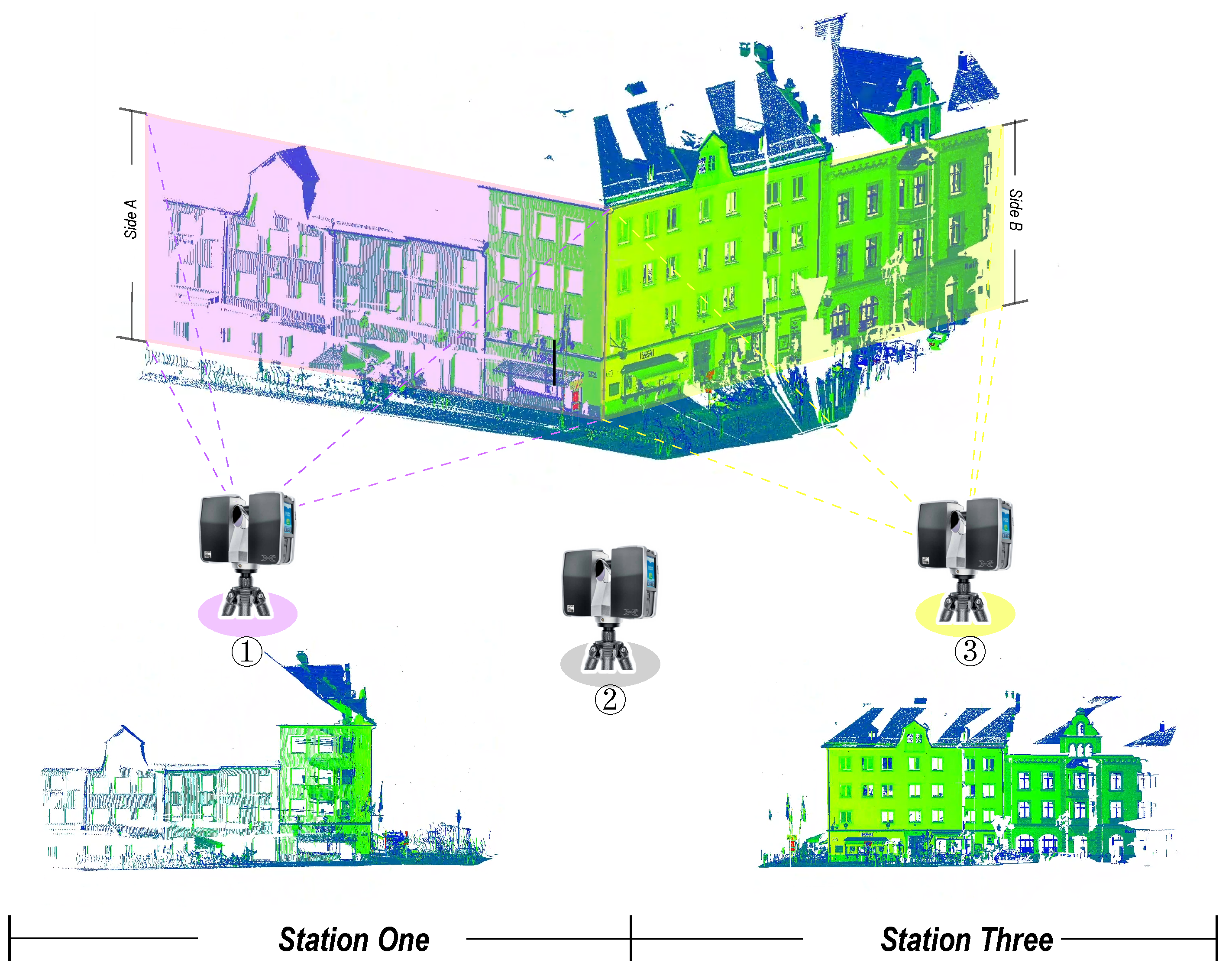
Figure 1. Datasets collected under different perspectives. Lidar systems are deployed at different sites to scan the same building, and datasets collected at each site are different. In general, the farther apart the sites are, the less overlap there is likely to be between the collected datasets.
Machines 11 00254 g001
Figure 2. Performance comparison of different algorithms. We conduct a comprehensive comparison of the different registration methods separately using processing time and alignment accuracy as the judging criteria. While some methods are faster in terms of processing time, others are more accurate. Collectively, our proposed approach achieves a balance between these two aspects and performs well in terms of both.
Machines 11 00254 g002
Figure 3. System workflow diagram. The system consists of four main components: (1) Data acquisition. As well as the drone-borne Lidar system and the TLS system, we also obtain data from third-party sources, such as Semantic 3D; (2) Data type. The data packages used include point cloud datasets and RGB image sets. There are different colors in the gradient bar (Machines 11 00254 i001) in the point cloud dataset that represent different altitudes; (3) Feature matching point pairs. A mixed feature pair point set is established through geometric matching and photometric matching; (4) Data processing. By optimizing random sampling and evaluation estimation, the RANSAC algorithm finally reaches target registration.
Machines 11 00254 g003
Figure 4. The whole process of 3D registration. The first step is to search and determine the respective feature points from the source and target point clouds based on their initial positions. According to the local features, the matching relationship between the feature points is further determined. Lastly, the feature points with the same name are transformed to the same position, and the point cloud is converted to the same coordinate system. (: Source Points, : Target Points, : Source Keypoints, : Target Keypoints, Machines 11 00254 i002: Correspondences).
Machines 11 00254 g004
Figure 5. Feature matching point set. The NARF and FPFH algorithms are used to extract 3D feature points from the laser point cloud data in the dataset, respectively, and the feature matching point pair set M g is established based on the local feature description method. The 3D feature points are then extracted using SIFT and the bilinear interpolation method for RGB images, which in turn generates the set of point pairs M p .
Machines 11 00254 g005
Figure 6. Scene classification. The main process and basic working principle of scene classification are introduced.
Machines 11 00254 g006
Figure 7. Acquisition system and on-site environment. (a) UAV-borne Lidar scanning system; (b) the location of the National Biathlon Ski Center for the Beijing Winter Olympics; (c) the collected color data.
Machines 11 00254 g007
Figure 8. Experimental sample selection. In addition to showing the full picture of the six sets of data, we also selected specific small samples for testing in the form of specific perspectives (Machines 11 00254 i003). Moreover, each small sample is displayed sequentially with laser point information and RGB image information. A gradient bar with a changing color based on the height is represented by Machines 11 00254 i004.
Machines 11 00254 g008
Figure 9. Comparison of registration effects of third-party data. On samples selected from third-party databases (Bird, Dom, and Sg27), we performed point cloud registration tests using RANSAC, FGR, NDT, GICP, NICP, and our proposed method. The dotted box represents the area of the image where there is an obvious deviation in registration, and the square represents the enlarged image of the local deviation.
Machines 11 00254 g009
Figure 10. Registration effect comparison. Bird, Dom, and Sg27 errors were measured with different methods using MSE, RMSE, and MAE as measurement indicators.
Machines 11 00254 g010
Figure 11. Comparison of registration effects for self-built data.On samples selected from self-built databases (SJC, CSC, and BSC), we performed point cloud registration tests using RANSAC, FGR, NDT, GICP, NICP, and our proposed method. There are two types of boxes in the figure: the dotted box represents the place where there is obvious registration deviation, and the solid rectangle represents an enlarged view of the local deviation.
Machines 11 00254 g011
Figure 12. Registration effect comparison. The errors of SJC, CSC, and BSC registered using different methods are measured using MSE, RMSE, and MAE metrics.
Machines 11 00254 g012
Figure 13. Registration time statistics. Time taken for different methods to process data.
Machines 11 00254 g013
Table 1. Lidar system parameters. In the process of acquisition, various parameters of the Lidar system are taken into consideration.
CategoryULSTLS
ModelDJI M600 pro+UAV-1 seriesFaro Focus 3D X130
Measuring Distance3–1050 m0.6–120 m
Scan Angle360°360° (horizontal), 300° (vertical)
Measurement Rate10–200 lines/s976,000 points/s
Angular Resolution0.006°0.009°
Accuracy±5 mm±2 mm
Ambient Temperature−10–+40 °C−5–+40 °C
Wavelength1550 nm1550 nm
Table 2. Platform configuration. A suitable test platform is selected whose software and hardware meet the requirements of the experiment.
CategoryConfiguration
SoftwareOperating SystemWin 11
Point Cloud Processing LibraryPCL 1.11.1
Support PlatformVisual Studio 2019
HardwareCPUIntel(R)Core(TM)i5-9400F
MemoryDDR4 32 GB
Graphics CardNvidia GTX 1080 Ti 11 GB
Table 3. Evaluation of results from third-party databases. Based on third-party test samples, we evaluated the performance of our method and other similar methods. (The ↓ indicates that the smaller the value, the better; bold indicates the best performance; underline indicates the second-best performance.)
MethodsMSE(R)↓RMSE(R)↓MAE(R)↓MSE(t) (× 10 2 )↓RMSE(t) (× 10 2 )↓MAE(t) (× 10 2 )↓
BirdDomSg27BirdDomSg27BirdDomSg27BirdDomSg27BirdDomSg27BirdDomSg27
RANSAC91.867174.33995.0759.58413.2039.7506.4838.5866.5800.0060.0370.0070.0770.1920.0830.0620.1160.065
FGR231.87974.285145.04915.2278.61812.0439.755.9197.9130.0020.0080.0020.0480.0930.0480.0320.0710.036
NDT15.9236.379208.8343.9902.52514.4513.1792.2539.3100.0020.0030.0320.0400.0510.1790.0260.0380.122
GICP4.70621.739118.7292.1694.66210.8962.0063.5867.2460.0010.0020.0020.0350.0410.0420.0250.0320.032
NICP2.8442.6992.7821.6861.6421.6681.6261.5861.6090.0310.0060.0030.1760.0790.0540.1050.0590.041
OURS1.7741.8596.5561.3321.3632.5611.1891.2532.2760.0010.0010.0010.0230.0370.0230.0180.0300.015
Table 4. Evaluation of the results of the self-built database. On the basis of our self-built test samples, we evaluated the performance of our method and other similar methods. (A smaller value indicates better performance, a bolded value indicates the best performance, and an underlined value indicates the second-best performance.)
MethodsMSE(R)↓RMSE(R)↓MAE(R)↓MSE(t) (× 10 2 )↓RMSE(t) (× 10 2 )↓MAE(t) (× 10 2 )↓
SJCCSCBSCSJCCSCBSCSJCCSCBSCSJCCSCBSCSJCCSCBSCSJCCSCBSC
RANSAC148.10776.56647.06212.1698.7506.8607.9865.9964.8900.1950.0660.0064.4132.5670.081.6420.7090.054
FGR41.707134.86632.8366.45811.6135.7304.6537.6634.2230.0398.4640.0021.98929.0930.0440.4452.4870.031
NDT17.8132.98616.4964.2211.7284.0613.3191.6773.2230.0320.0190.0011.7981.3940.0260.2020.2840.018
GICP2.94734.9332.5961.7165.9101.6111.6534.3301.5560.0040.0490.0010.6362.2070.0320.7590.5400.027
NICP9.8671.99363.9563.1411.4117.9972.6731.3285.5680.0120.0040.0341.0970.1760.1850.8150.1450.123
OURS1.6671.9302.4361.2911.3891.5611.0131.2961.5060.0010.0030.0010.0180.1790.0230.0040.1200.015
Table 5. Time consumption comparison. Various methods are used sequentially to register selected samples, record the respective time, and analyze the results. (There is an indication of the best performance in bold, while there is an indication of the second-best performance in underline.)
MethodsTime(s)
BirdDomSg27SJCCSCBSC
RANSAC46.29331.58465.79143.62655.41830.084
FGR76.57560.52778.61464.57150.00854.225
NDT89.402124.051166.569103.36688.62963.748
GICP94.03584.504108.60877.54780.64466.313
NICP80.22435.27170.54748.51461.52238.693
OURS48.66928.05362.18146.29648.15825.466
Disclaimer/Publisher’s Note: The statements, opinions and data contained in all publications are solely those of the individual author(s) and contributor(s) and not of MDPI and/or the editor(s). MDPI and/or the editor(s) disclaim responsibility for any injury to people or property resulting from any ideas, methods, instructions or products referred to in the content.