Article

A Multi-Task-Based Deep Multi-Scale Information Fusion Method for Intelligent Diagnosis of Bearing Faults

1
School of Information and Control Engineering, Jilin Institute of Chemical Technology, Jilin 132022, China
2
School of Science, Jilin Institute of Chemical Technology, Jilin 132022, China
3
School of Software, Jilin University, Changchun 130015, China
*
Author to whom correspondence should be addressed.
These authors contributed equally to this work.
Machines 2023, 11(2), 198; https://doi.org/10.3390/machines11020198
Submission received: 9 December 2022 / Revised: 10 January 2023 / Accepted: 11 January 2023 / Published: 1 February 2023
(This article belongs to the Special Issue Advances in Machinery Condition Monitoring, Diagnosis and Prognosis)

Abstract

:
The use of deep learning for fault diagnosis is already a common approach. However, integrating discriminative information of fault types and scales into deep learning models for rich multitask fault feature diagnosis still deserves attention. In this study, a deep multitask-based multiscale feature fusion network model (MEAT) is proposed to address the limitations and poor adaptability of traditional convolutional neural network models for complex jobs. The model performed multidimensional feature extraction through convolution at different scales to obtain different levels of fault information, used a hierarchical attention mechanism to weight the fusion of features to achieve an accuracy of 99.95% for the total task of fault six classification, and considered two subtasks in fault classification to discriminate fault size and fault type through multi-task mapping decomposition. Of these, the highest accuracy of fault size classification reached 100%. In addition, Precision, ReCall, and Sacore F1 all reached the index of 1, which achieved the accurate diagnosis of bearing faults.

1. Introduction

Rolling bearings play an important role in industrial equipment [1]. Failures in rolling bearings are usually characterized by abnormal vibrations caused by regular changes in the stiffness of the rotating system [2,3]. Bearing defects account for 40% of failures in large mechanical systems and 90% in small automated systems [4]. Rolling bearings control the risk of mechanical equipment failure, effectively improve the continuity and reliability of the regular operation of rotating bearings and mechanical equipment, and reduce operation and maintenance costs. There is an urgent need to conduct in-depth research on intelligent condition monitoring and fault diagnosis of rolling bearings, understand their degradation process, monitor the degree of failure and damage, and determine the damage location. Ultimately, this will serve as an essential basis for maintenance solutions.
The four main components of the rolling bearing fault diagnosis process are signal pre-processing, feature extraction, feature selection, and pattern classification [5]. Signal pre-processing can expand the fault features of small samples and reduce noise interference in the data acquisition process [6]. Feature extraction filters out useful critical information and removes invalid or redundant information such as noise, which is a crucial step in distinguishing the health of a diagnostic object [7]. Feature selection is to select the signal with strong fault expression capability by splicing and fusing the information after feature extraction [8]. Pattern classification obtains the classification results after feature selection using a classifier to derive the fault category information of rolling bearings [9]. Through research, the published literature now contains many bearing fault diagnosis techniques, which generally can be divided into model-driven and data-driven-based techniques [10].
Based on model-driven technology, it is necessary to extract the characteristic quantities of the health status of mechanical equipment with rich prior knowledge and then diagnose them according to the corresponding intelligent algorithm. For example, Lei et al. [11] used empirical modal decomposition to extract multi-order eigenmode function vectors. They then used the Hilbert transform to obtain spectral information to extract the features of normal and fault signals. Liu et al. [12] used multiple fractal detrending interrelation analysis and the EMD method to extract non-linear information from different fault states. This can obtain more fault information for rolling bearing fault diagnosis [13,14]. However, these techniques are too complex, require a lot of manual operations, and are only applicable to specific parameters of mechanical equipment, making them less universal and generalizable [15], thus hindering their widespread use in industry.
Data-driven techniques based on data can be used to map the relationship between data and fault types by mining the descriptive connections and information about the equipment from a large amount of historical data. This technique enables the extraction of fault feature information from complex vibration signals without excessive a priori knowledge and harrowing manual extraction [16]. Due to the advantages of flexible structural adjustment and firm performance in adaptive extraction of information, deep learning techniques have better representation than traditional pattern-driven extraction of features. Convolutional neural networks are currently widely used in deep learning. For example, Fuan W et al. [17] proposed a parameter adaptive CNN model and applied it to fault diagnosis, which can adaptively determine the main parameters in the network. Zhang et al. [18] used a convolutional neural network structure to design a WDCNN model to recognize the collected bearing vibration signals directly. The WDCNN model achieved 100% recognition rate for normal signals. Zhang D et al. [19] attempted to combine CNN with a migration learning approach for fault identification in rolling bearings. The CNN model was first trained using a grey-scale map, and the parameters from the original CNN were then passed to DCNN-TL to complete the fault diagnosis. Kumar A et al. [20] first subjected the vibration signal to a continuous wavelet transform and then used CNN to classify it, eventually achieving good recognition results.
From the existing literature on the application of convolutional neural networks to bearing fault diagnosis, it can be seen that it is difficult for a single CNN model to comprehensively extract fault feature information, and the use of a multi-scale CNN model structure can obtain comprehensive feature-sensitive information from different perspectives. The adoption of attention mechanism can dynamically adjust the weight distribution of different feature information, which makes the prediction accuracy of the model higher and more stable. Therefore, to meet the requirement of acquiring fault feature information accurately and effectively, this paper proposes an intelligent bearing fault diagnosis method based on a multi-tasking deep multi-scale information fusion model (MEAT). The proposed MEAT model is capable of capturing different levels of information from multi-scale CNNs and using attention mechanism to dynamically weight the obtained fault features and fuse the weighted features. Adding a multi-task disassembly strategy to the fault diagnosis process, the diagnosis of fault types and fault sizes can be done in parallel. In addition, the sub-models can be flexibly migrated and applied.
  • A training strategy of task splitting was proposed to achieve fault-type diagnosis and size localization simultaneously. By splitting fault diagnosis multi-tasking into fault size tasks and fault type tasks, the model can flexibly adjust the weights of subtasks to balance the convergence speed. In addition, it can also apply local models of subtasks to other research objects to enhance the models’ robustness while improving the models’ transferability.
  • Multi-scale convolution was used for feature extraction to obtain different levels of fault information. This allowed feature extraction of the original data from different perspectives, reducing the limitations of single-scale convolution for feature extraction of time-series data, and making the extracted features more comprehensive and conducive to the following information fusion step.
  • A multi-layer attention dynamic weight assignment strategy for multi-scale convolutional neural networks was proposed to weight and fuse the fault features. The system uses the first layer of attention to dynamically weight the feature vectors obtained by convolution at different locations, and the model can assign greater weights to necessary periods. In addition, since the first layer uses multi-scale convolution, the granularity of information obtained by different scale convolution is different. It is also important. Again, the second layer uses attention to weight the information extracted under different information granularity, thus significantly improving the model prediction capability.
  • A multi-block model structure was proposed to improve the model’s prediction accuracy. More extensive and complementary features are extracted within each block through feature transfer. At the same time, the model utilizes multi-layer attention to assign weights to elements through dynamic weight assignment and uses parameter sharing to pass the weighted feature matrix to the next block as hidden layer information. To achieve higher latitude of information extraction, the higher the freedom of information extraction, the better the prediction effect.
This paper is structured as follows. Section 2 and Section 3 describe the proposed method. Section 4 analyzes and discusses the experimental results of the proposed model on the CWRU-bearing dataset. Finally, Section 5 concludes the paper.

2. Related Works

2.1. Convolutional Neural Network

The CNN is a neural network with multiple feedforward layers, which has excellent learning and feature extraction capabilities, including a filtering stage and a classification stage. The filter stage can be used to extract features, while the classification stage can be used to classify the patterns of the extracted fault features [21]. The filter stage consists of convolutional layers, pooling layers, and other basic units, while the classification stage generally consists of fully connected layers.
In this experiment, we used the convolutional kernel scale of 2 as an example to illustrate the classical CNN structure. The input data of the convolutional model used in this paper was 8 × 9 × 5 , the dimension of the convolution layer was 8 × 9 × 64 , the dimension of the pooling layer was 4 × 4 × 64 , and the dimension of the fully connected layer was 1024. The model structure of the convolutional neural network is shown in Figure 1.
The convolutional layer performs feature extraction on the input one-dimensional time series signal. Convolutional kernels are used to perform convolutional operations on local regions of the input signal, and local features are extracted from the local regions by these kernel functions [22]. The specific convolutional layer operation is shown in the following equation,
y l ( i , j ) = K i l × X l ( r j ) = j = 0 W 1 K i l ( j ) X l ( j + j )
where y l ( i , j ) is the dot product of the kernel, and the local area, K i l ( j ) is the first weight of the convolution kernel in the first layer, X l ( r j ) is the first convolved local region in the first layer, and W is the width of the convolution kernel.
In this experiment, since time-series data were used, the convolution operation was also along the time-series direction. Its width was kept consistent with the vector dimension of the time-step mapping. Multi-scale convolution was adopted in the convolution layer, where separate convolution kernels of different sizes were used to convolve the original data.
The pooling layer was used to compress the extracted feature maps and keep the feature scale constant. Ref. [23] Mean pooling takes the mean value of the neurons in the perceptual domain as the output value, so mean pooling was weighted with equal weights. The following equation gives the mathematical description,
p l ( i , j ) = 1 W t = ( j 1 ) W + 1 j W a l ( i , t )
where a l ( i , t ) is the value of the t th neuron in i th framework of layer l and t ϵ [ ( j 1 ) W + 1 , j W ] , W is the width of the pooling size, and p l ( i , j ) is the corresponding value of the neuron in layer l of the pooling.
In this experiment, the traditional pooling layer was replaced with a hierarchical attention structure. The fusion process of attention is a weighted pooling process. It gives different weights according to the contribution of features extracted by different scales of convolution to the result, in order to enhance compelling features, weaken invalid or redundant features, and increase the accuracy of classification, as detailed in Section 3.2.
Fully connected layers were used for the integration of high-dimensional features. Its final layer was the output classification layer.

2.2. Batch Normalization

In training a neural network, normalizing the data can reduce the shift of internal covariates, thereby speeding up the training speed of the network and solving the problem of gradient dispersion. By stabilizing the mean and variance of the activation function’s input variables, the Batch Normalization layer can help relieve the pain of Internal Covariate Shift [24]. In addition, the neural network applying Batch Normalization has an excellent gradient flow in backpropagation. The initial and scale dependence of the neural network on the weights is reduced, making the learning more efficient and reducing the risk of non-convergence. The specific BN operation is shown in the following equation,
z l ( i , j ) = γ l ( i , j ) y ^ l ( i , j ) + β l ( i ) , y ^ l ( i , j ) = y l ( i , j ) μ σ 2 + ε
μ = 1 n i = 1 n y l ( i , j )
σ 2 = 1 n i = 1 n ( y l ( i , j ) μ ) 2
where z l ( i , j ) represents the output of a neuron, and γ l ( i ) and β l ( i ) are the scale and shift parameters to be learned, respectively, μ and σ 2 in normalized y ^ l ( i , j ) are the mean and variance of y l ( i , j ) ,   and   ε is a small constant to prevent invalid calculations when the variance is 0.

2.3. Attention Mechanism

The attention mechanism can be regarded as a general structure of Encoder-Decoder, while the attention function can be described as mapping a query and a set of key-value pairs to an output, where query, keys, values, and production are all vectors [25]. The essence of attention is to assign a weight coefficient to each part in the data sequence. If each component of the series is stored in (k, v), then attention completes the addressing by calculating the similarity between the query and keys. The attention score is the similarity derived by the question and the keys, which shows the relevance of the extracted data, i.e., the weight, and then the attention value is calculated by weighted summation [26].
We assumed that the input query’s dimension and the key were d k , and the size of values were d v . We then calculated the dot product of the query and each key, divided by d k and applied the Softmax function to calculate the weights [27]. In the actual operation process, the question, keys, and values were processed as matrices Q , K , V , respectively, and the output matrix was obtained as:
A t t e n t i o n ( Q , K , V ) = s o f t m a x ( Q K T d k ) V
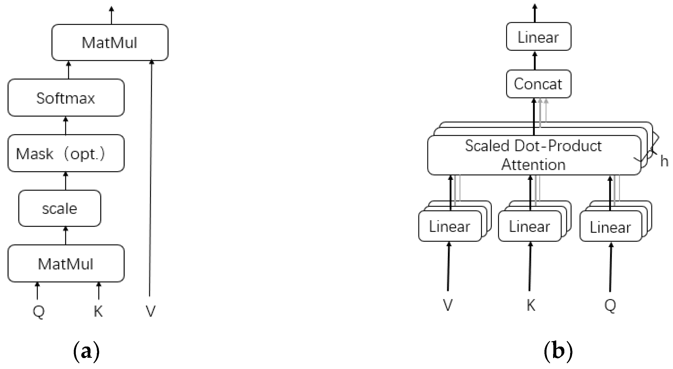
The attention in the proposed model adopted multi-head attention. In the single attention mechanism, due to the existence of the mean-taking operation, the representation information in different subspaces at different locations was discarded by the model, and the single attention only performed attention operations on K , Q , and V . Multi-head attention can combine the information learned from different head parts, which can be effectively obtained by multiple linear mapping of each dimension of K , Q , and V . It can also be regarded as stacking of scaled dot-product attention.
Scaled dot-product attention is our commonly used attention that uses dot product for similarity calculation, except that one more d k (the dimension of K ) is adjusted so that the inner product is not too large [28]. Figure 2a shows the structure of scaled dot-product attention.
The multi-head attention structure is shown in Figure 2b. Q , K , and V were first fed into a linear transformation and then input to the deflated dot product attention, and after repeatedly performing h attention operations, the obtained results were spliced and the value obtained by another linear transformation was used as the result of multi-head attention [29]. Here the hyperparameter h was the number of heads, and its embedding dimension was partitioned into h copies, and h heads represented h different representation subspaces, and different meanings were learned by different representation subspaces. Moreover, the parameters W were not shared for each linear transformation of Q , K , and V . Using a multi-head attention model can jointly pay attention to the representation information of different representation subspaces at different locations,
M u l t i H e a d ( Q , K , V ) = C o n c a t ( h e a d 1 , , h e a d h ) W O
w h e r e   h e a d i = A t t e n t i o n ( Q W i Q , K W i K , V W i V )
where the matrices are W i Q d m o d e l × d k , W i K d m o d e l × d k , W i V d m o d e l × d v and W i O h d v × d m o d e l .
In this experiment, we used parallel attention layers or heads with h = 10. For the data of different segmentation lengths L obtained from different sliding windows for each head (head) in the experiment, the scale of each head (head) was determined by s c a l e = s p r t ( L / / h ) .

3. The Proposed Method

3.1. Feature Extraction Based on Single-Layer Attention

The attention mechanism is a series of attention allocation coefficients, which can identify the essential parts of the current output from the complex input information, which is simply weighted. In terms of the model, attention is generally used in CNN and LSTM. The convolution operation of ordinary CNN can extract essential features, but the convolutional field is local, and it needs to expand the field of view by stacking multiple convolutional areas [30]. In contrast, the attention operation between convolutions can expand the perceptual lot of the convolutional layers, which makes the local saliency information have a higher weight.
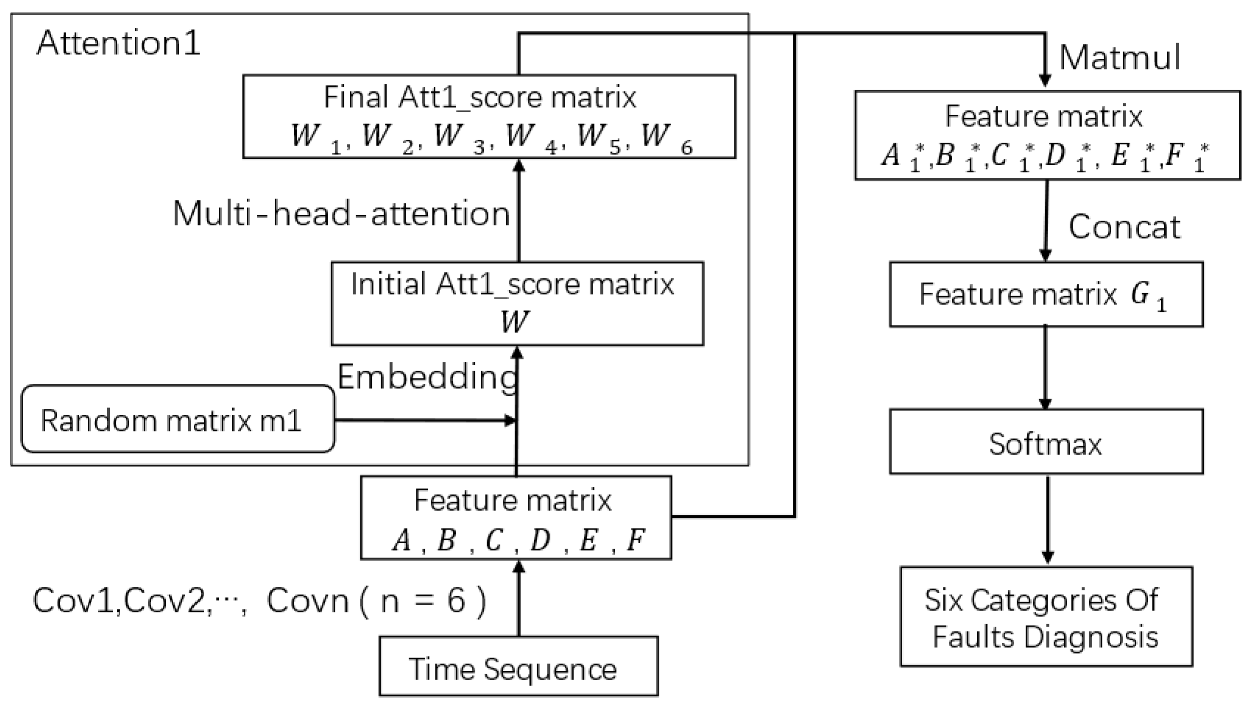
This research used multi-scale convolution as the primary model for bearing fault diagnosis. The model structure for feature extraction by the single-layer attention convolution model (SLAT) is shown in Figure 3. First, the time series dataset preprocessed by the data was convolved by six convolutional layers of different scales to achieve feature extraction of the original data, where the size of the convolutional kernel was 1, 2, 3, 4, 5, 6, and the corresponding six feature matrices ( A , B , C , D , E ,   F ) were obtained after convolution, and then the initial attention score matrix w   was obtained by embedding a model randomly generated weight matrix m 1 . Secondly, the weighted attention matrices ( w 1 , w 2 , w 3 , w 4 , w 5 , w 6 ) were weighted by the multi-head attention mechanism, and the weighted feature matrices ( A   * , B   * , C   * , D *   , E   * , F   * ) were obtained by multiplying them with the six initial feature matrices, and the dimension of the matrix was 8 × 1 × 100 . Finally, the weighted feature matrix was stitched by Concat to get the feature matrix G 1 , the dimension of the matrix was 8 × 6 × 100 , and the diagnosis results were obtained by direct classification in the Softmax layer.
The model aimed to extract valuable features by giving different weights to the features extracted by convolution at different scales according to different attention angles. The pseudocode of the algorithm is shown below:
Algorithm 1: Feature Extraction Based on Single-Layer Attention.
Input Parameters: FeatureMatrix (A, B, C, D, E, F); RandomMatrix (m1); HidDim (Dim); Head (h)
Result: FeatureMatrix (G1)
W = Att1_scoreMatrix (m1)
For I in FeatureMatrix (A, B, C, D, E, F);
   q = Linear (Dim);
   K = Linear (Dim);
   v = Linear (Dim);
   Scale = sqrt (Dim//h)
   Q = q (I).view (m1.shape [0], −1, h, Dim//h).permute(0, 2, 1, 3);
   K = k (I).view (m1.shape [0], −1, h, Dim//h).permute(0, 2, 1, 3);
   V = v (I).view (m1.shape [0], −1, h, Dim//h).permute(0, 2, 1, 3);
   FinalAtt1_scoreMatrix (W1, W2, W3, W4, W5, W6) = Q * KT/scale;
   x = matmul (softmax (FinalAtt1_scoreMatrix), V);
   FeatureMatrix (A1 *, B1 *, C1 *, D1 *, E1 *, F1 *) = x. permute (0, 2, 1, 3).view (m1.shape [0], −1, h * Dim//h);
FeatureMatrix (G1) = Concat. FeatureMatrix (A1 *, B1 *, C1 *, D1 *, E1 *, F1 *)
end

3.2. Feature Fusion Based on Multi-Layer Attention

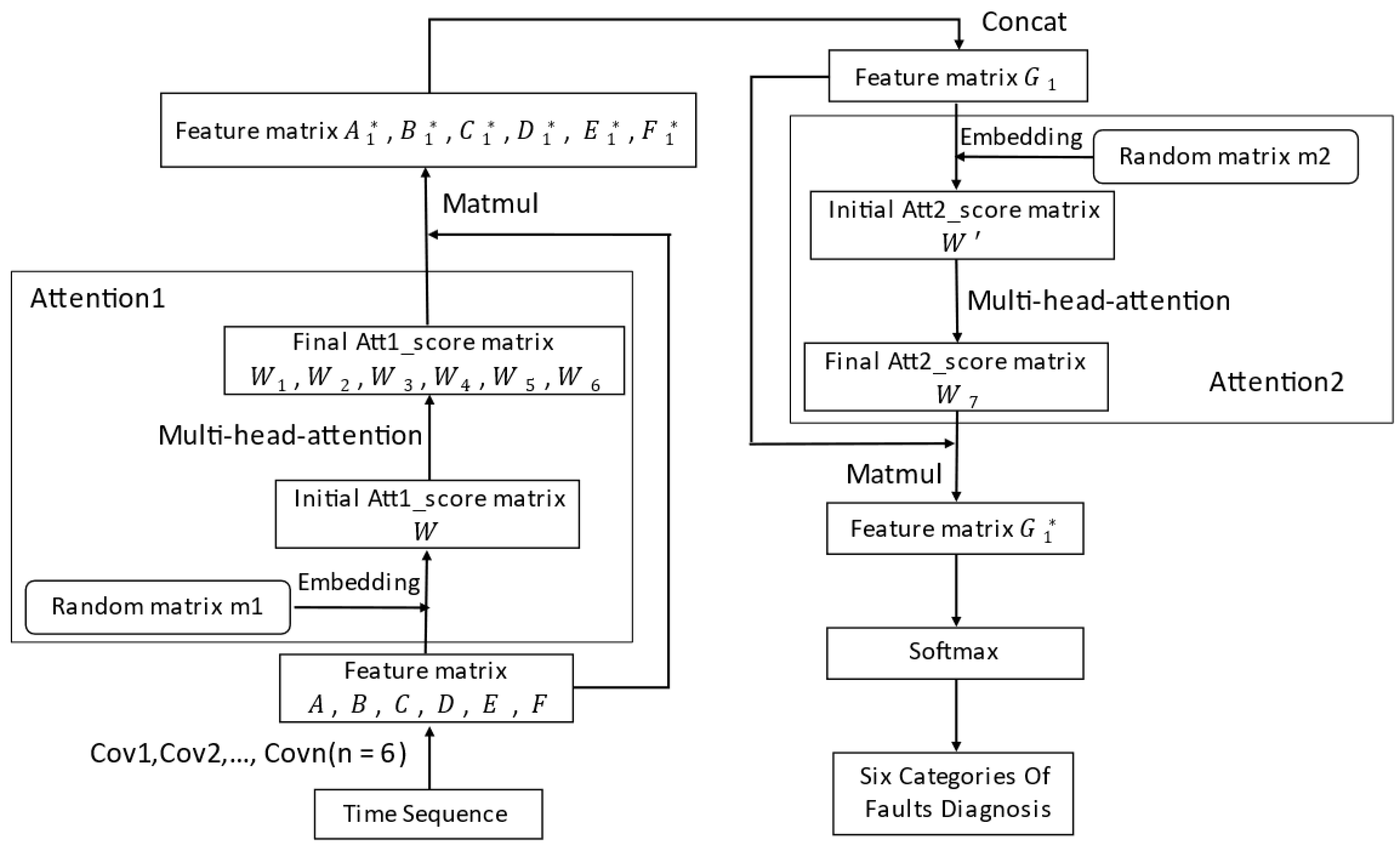
The multi-layer attention convolution model (MLAT) improves the single-layer attention convolution model (SLAT). MLAT uses a multi-layer multi-head attention mechanism in the model framework and performs attention-weighted fusion after the SLAT has been extracted by convolution at different scales. The parameters of each layer of attention are independent of each other. Since the size of the convolution kernels used in SLAT varies, and the convolution results contribute differently to the model, attention weighting was again used in the model for feature fusion. The structure of the MLAT model for feature fusion is shown in Figure 4. The initial attention score matrix w’ was obtained by first embedding the feature matrix G 1 in the SLAT model with a model randomly generated weight matrix m 2 , and then the score matrix was processed by the multi-head attention mechanism to obtain the weighted attention score matrix w 7 , and finally the score matrix w 7 and the feature matrix G 1 were multiplied to obtain the feature matrix G 1   * , the dimension of the matrix was 8 × 1 × 100 , which was then directly classified by the Softmax layer to obtain the diagnosis results. The MLAT model addressed such problems as the existence of certain differences in the merits of features after convolution at different scales. The spliced feature matrix was then further weighted by the second layer of the multi-head attention mechanism for feature fusion, and compared with the feature matrix G. The final resulting feature matrix G* deflated the effective and redundant features in the fused information once again, so that the model identified the features with a stronger ability to characterize faults in the weighted fusion process.

3.3. Multi-Tasking Pattern Classification

Single-task learning refers to simple top-to-bottom control flow execution and may ignore information that helps optimize a metric. Multi-task learning allows our model to generalize the original task better by sharing representational information between related jobs. Multi-task learning is also a transfer learning algorithm that trains multiple tasks in parallel using shared symbolic information. The primary goal is to improve generalization by exploiting domain-specific information implicit in the training signals of various related studies [31].
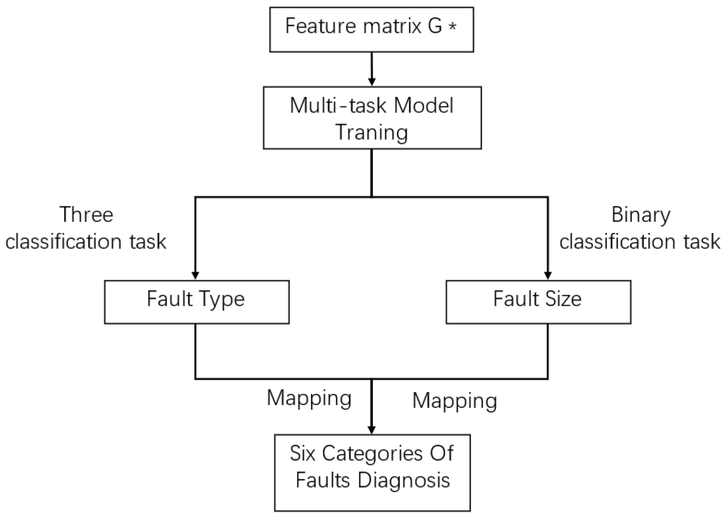
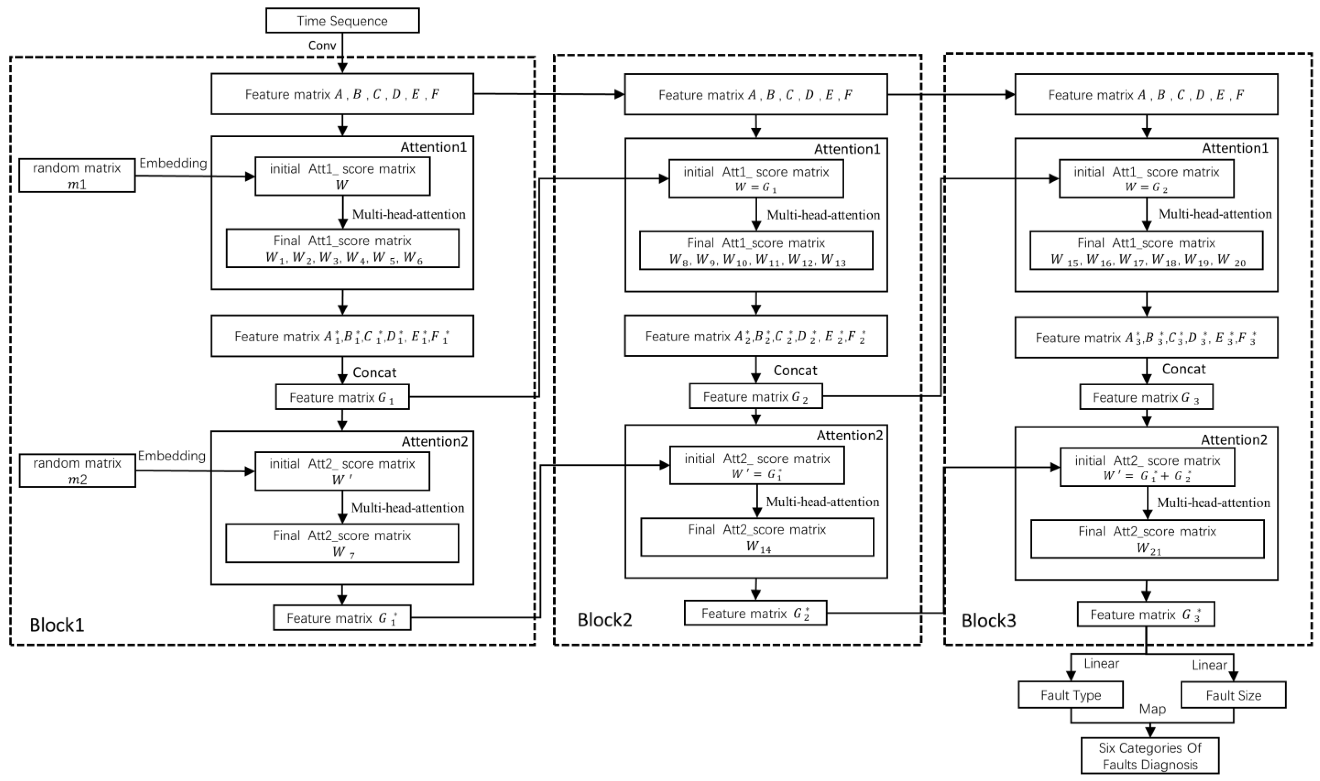
The single task convolution model (STAT) referred to the direct six classifications after obtaining the feature matrix G* by Softmax. The multi-task convolution model (MTAT) structure is shown in Figure 5. The feature matrix G* in MTAT was not directly classified by Softmax and was divided into two sub-tasks for execution. The subtasks were a fault type for a triple classification task and a fault size for the binary classification task. After the two subtasks had been predicted and classified, the experimental results were mapped back to complete the fault diagnosis six-classification task. For example, in our experiments, two subtasks diagnosed bearing faults as B, I, O, and 7, 14 respectively, and the mapping to the six classifications of bearing faults after completing the predictive classification of the two subtasks was B7, B14, I7, I14, O7, O14. In addition, MTAT also reduced the amount of training data required as well as improved the generalization ability of the model by migrating some or all of its knowledge to a related task after completing one of the subtasks.

3.4. Multi-Block Learning Structure

In Section 3.2, this paper proposes a multi-layer attention convolution (MLAT) based model to achieve better classification by learning the weights by itself. This model structure is a single-block structure. Inside the single block, different feature information is extracted from the time series dataset by multi-scale convolution at the beginning of each period. Then the convolved features are weighted by the first layer multi-head attention mechanism. The feature matrix G is obtained by stitching and fusion using Concat, which amplifies the practical features and reduces the useless features. The fused feature matrix G is then weighted by the second layer multi-head attention mechanism for the results extracted from the different convolution scales. The feature matrix G* is obtained by feature selection of the fused features. The weighted feature matrix G* is the final feature matrix of the single-layer block. If only one block layer is used, this feature matrix can be used as the classification matrix.
This sub-section of the paper describes a 3-layer block structure for data processing, where the feature information from the block in the previous layer was input to the block in the next layer. Firstly, the feature matrices A, B, C, D, E, and F from the previous block after multi-scale convolution were used as input to the next layer. Secondly, the initial score matrices w   and   w of the two layers of attention in the first block were obtained by embedding initialization. In contrast, the initial score matrix of the multi-layer attention in the second layer block was obtained from the result w = G 1 and w = G 1   * of the attention in the first layer block. The initial score matrix of the multi-layer attention in the third-layer block was obtained from the results of attention w = G 2 and w = G 1   * + G 2   * in the first and second-layer blocks. We demonstrated experimentally that this model of progressively passing parameters to the next layer allows for greater access to more abstract and valid information. The multi-block structure is shown in Figure 6.
This section illustrates how multi-block works with a 3-layer block; Block1, Block2, and Block3 are related by name.

4. Experimental Verification

4.1. Datasets Introduction

The experimental data used were obtained from the Case Western Reserve University (CWRU) Bearing Data Centre [32]. The test stand collected vibration signals at a rate of 12,000 samples per second from sensors mounted on the drive and fan side of the motor. In this dataset, four types of faults were provided by machining different fault sizes at different locations on the inner ring, outer ring, and ball body. The fault data were recorded at a sampling frequency of 12 kHz and a speed of 30 Hz. Six test conditions were considered, containing three different fault modes and two different fault sizes, which are described in Table 1. The six fault categories are named B7, I7, O7, B14, I14, and O14, and the data for each fault type contained 120,000 data points.
In the data pre-processing process, samples with different cut lengths were obtained by changing the size of the sliding window to get other data point numbers. Nine data samples with varying cut lengths, of 100, 200, 300, 400, 500, 600, 800, 1000, and 1200, were selected for the experiment. The sample data were combined into a data matrix, and the data samples were then divided equally into three parts. Two parts were used as the training sets and one part as the test set, and the experiments were conducted using the tri-fold cross-validation method. The original time and frequency signals of the six fault categories listed in Table 1 were subjected to FFT processing to obtain the time-frequency diagrams, as shown in Figure 7, for the ball fault B7 with 0.007 mil damage.

4.2. Ordinary Convolutional Model vs. Single-Layer Attention Convolutional Model

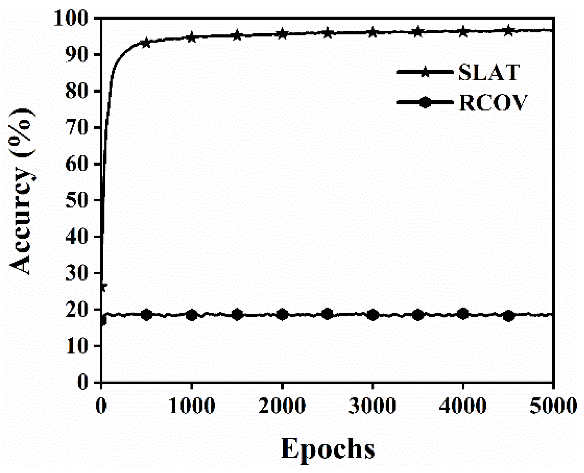
When predicting classification results based on the ordinary convolutional model (RCOV), a single-layer attention convolutional model (SLAT) was constructed for feature extraction after the convolutional results were weighted by the attention mechanism to improve the neural network’s ability to express the model. From Table 2, it can be seen that the highest accuracy was achieved when the cut length was 1200, so this was determined as the optimal SLAT cut length. From Figure 8, it can be seen that the highest accuracy (acc) of the ordinary convolutional model (RCOV) without attention weighting was 23.3%. The highest accuracy (acc) of the single-layer attention convolutional model (SLAT) with the optimal cut length of 1200 was 97.5%. The model’s accuracy reached 90% for the first time in the 223rd round. Compared with the RCOV model, the SLAT model had high accuracy and high-speed model fitting, effectively extracting features with strong characterization performance and eliminating redundant features by attention weighting. Moreover, the accuracy of the test set was higher than the accuracy of the training set, and the model had better generalization ability.

4.3. Comparison of Single-Layer Attention Convolution Model and Multi-Layer Attention Convolution Model

To improve the model prediction classification results, the multi-layer attention convolution model (MLAT) proposed in this paper was obtained by improving on the single-layer attention convolution model (SLAT). Six classification experiments were conducted on this model, and 3-fold cross-validation was taken to get the final prediction results.
From Table 3, it can be seen that the cut length of sample data affected the model’s performance. The cut length with the highest accuracy in both SLAT and MLAT was 1200, and it can be seen from the data in the table, that the longer the sample cut length was, the higher the accuracy of the model and the more robust it was.
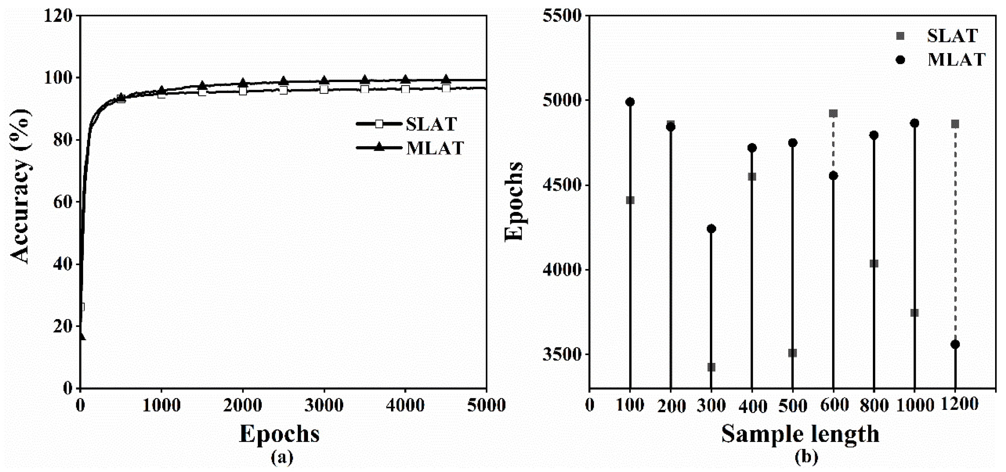
From Figure 9a,b it can be seen that the highest accuracy (acc) of the SLAT model was 97.5% under the optimal cut length of 1200, and the optimal result was reached at the 4860th round; the highest accuracy (acc) of the MLAT model was 99.66%, and the optimal outcome was achieved at the 3560th round. Compared with the SLAT model, the MLAT model had higher accuracy. The feature fusion using the multi-layer attention convolution model made the model fit faster and improved the generalization ability of the model.
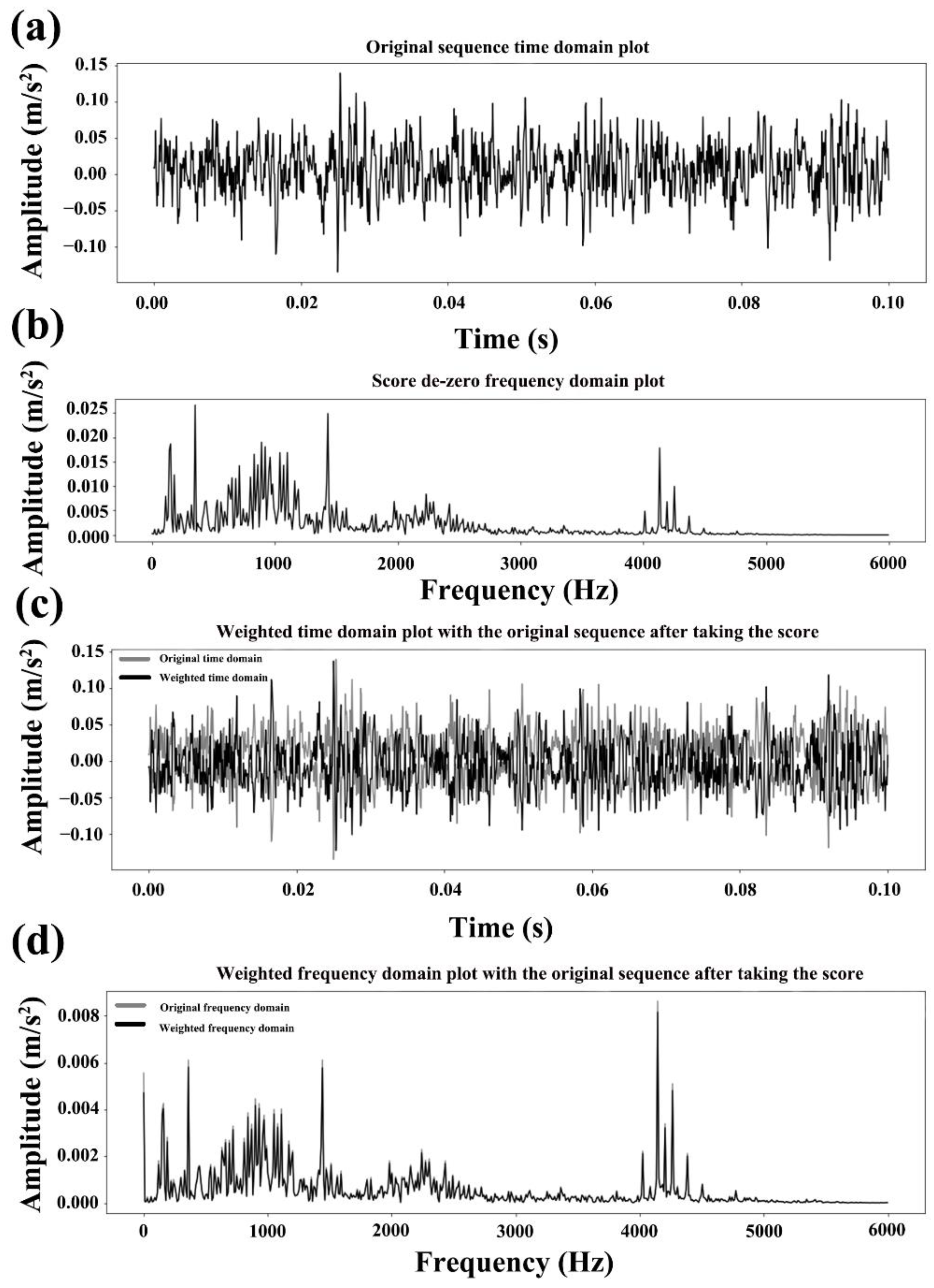
This paper shows in Section 4.1 the time-frequency domain features of fault signals obtained by Fast Fourier Transform (FFT). We verify the model classification accuracy by comparing the time-frequency domain features of faults obtained by signal processing methods and model classification methods. To visualize the process of model weighting, the inverse weights of the trained model were explored. The weighting results of the first layer of attention under the corresponding convolution were obtained.
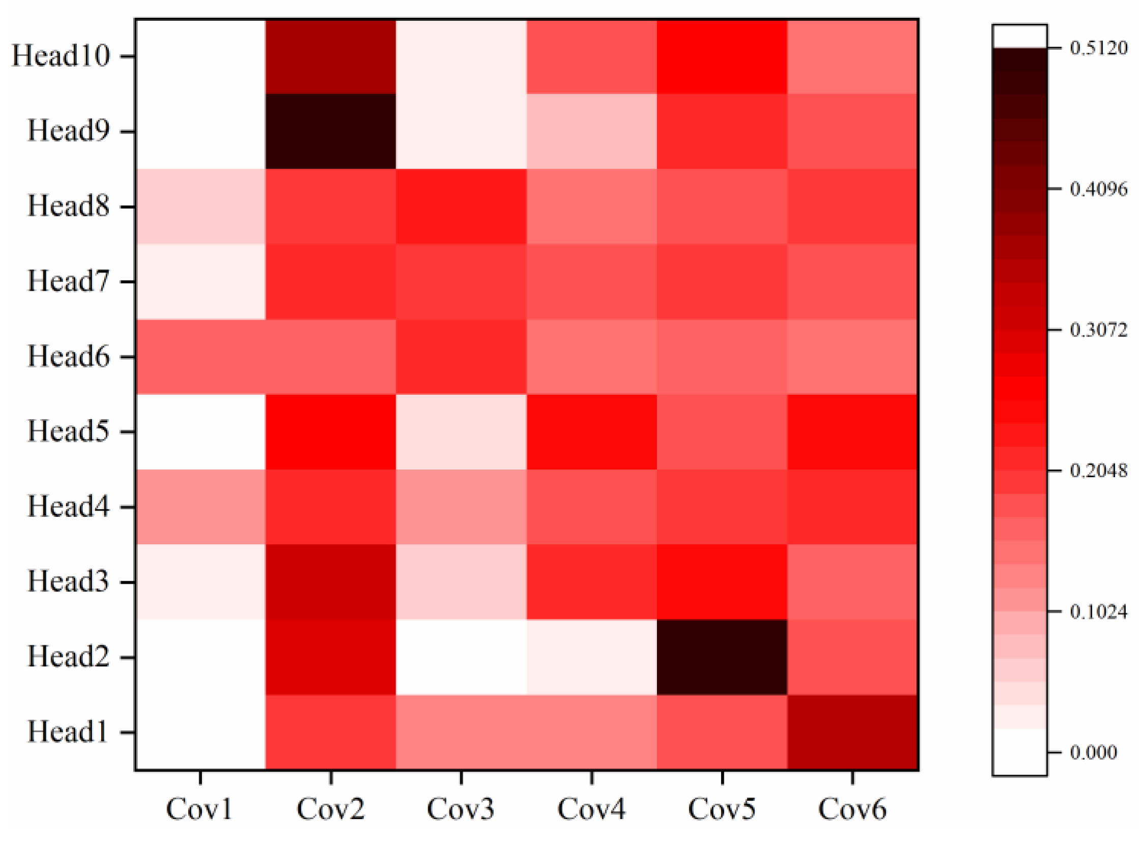
Firstly, the weight values of the second layer attention were extracted, and the second layer attention resulted in a matrix of 10 × 6, where 10 denotes the multi-headed attention mechanism’s 10 heads (10 different attention angles), and 6 represents the convolutional scales of 1, 2, 3, 4, 5, and 6, respectively; the results are shown in Figure 10. From the figure, it can be seen that the darker the color block, the greater the weight value. The results of 10 heads are averaged in the last row to obtain the results with the enormous weights containing convolutional scales of 2, 5, and 6. For the 3-scale convolution, although the average result is not high, three heads took the maximum weight; therefore, further exploration was conducted.
The optimal weights were obtained from the second layer weight results under the convolution scale of 2, 3, 5, and 6; therefore, the weight results of the first layer attention under the corresponding convolution were obtained in turn, and the first layer attention weight results were obtained as a discounted graph. Take the convolution scale equal to 2 as an example, as shown in Figure 11. The optimal weights were generally the group with the most prominent peak in the folded graph, and the optimal weight results were selected for exploration. According to Figure 11, it can be seen that the group with the most significant peak fluctuation was the 4th head, and the group with the most significant peak fluctuation was the 10th head, so the optimal weight under the 2 scales was the 4th head.
The development of the 4th head of the optimal weight under the 2 scales in the single-layer attention convolution model was extracted. The score was calculated by the inverse of the formula ln ( 1 / ( x 1 ) . The score result was weighted to the original sequence, and the result is shown in Figure 12.
After the frequency domain transformation of the weights, the maximum frequency bands of the frequency domain results of the score removed from 0 and the original sequence were concentrated in 0–2000 Hz and 4000 Hz–5000 Hz, indicating that the size of the weights was closely related to the validity of the features in the feature weights given by the model. The consequences were deflated for the features based on the abstract information in the original data. According to Figure 12, after the weighting of the score and the original sequence, and the original sequence was compressed to the same interval, the time-domain and frequency-domain plots matched. The weighted frequency-domain results fluctuated less, indicating that the weight allocation ratio and the fault location search model were based on the original data, which corresponded entirely to the search results.

4.4. Single-Task vs. Multi-Task Comparison of Multi-Layer Attention Convolution Models

The multi-task convolutional model (MTAT) proposed in this paper was obtained by improving based on the single-task convolutional model (STAT) to improve pattern classification accuracy. Two subtasks were composed from the perspective of fault type and fault size to complete the model prediction classification process. Compared with the traditional single-task convolutional model (STAT) for direct six-classification tasks, the multi-task convolutional model (MTAT) pattern classification was transformed into a fault type three-classification task and a fault size two-classification task.
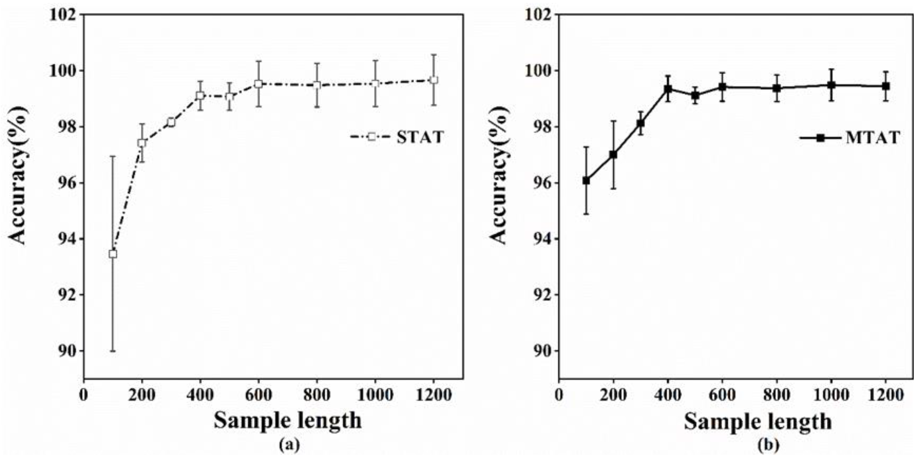
From Table 4, the cut length with the highest accuracy in MTAT was 1200; therefore, 1200 was determined as the optimal cut length in MTAT. From Table 4, and Figure 13a,b, the highest accuracy (acc) of the single-task model was 99.67%, and the average accuracy (acc) of the single-task model was 98.38%; the highest accuracy (acc) of the multi-task model was 99.49%, and the average accuracy (acc) of the multi-task model was 98.60%. The difference between the maximum accuracy of single-task and multi-task was minimal. However, the average accuracy of the multi-task model was higher, the deviation of each group of data from the overall data mean was smaller, the model was more stable, and the fitting speed was faster.
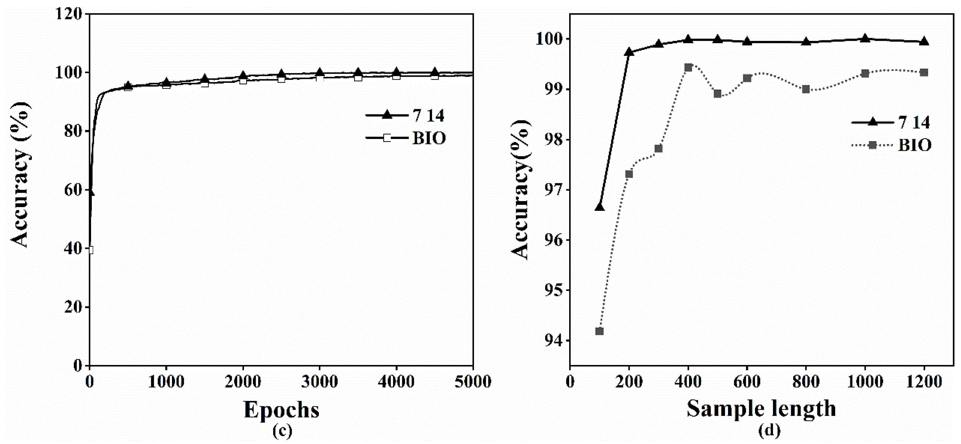
From Table 5, and Figure 13c,d, the two subtasks in the multi-task model achieved high classification accuracy under the optimal cut length of 1000 and the model’s performance under different subtasks was very superior. The highest precision (acc) was 99.43% for the fault type task (BIO) and 100% for the fault size task (7, 14) for the subtasks at different sample lengths, and the two subtasks were parallel and independent. Both can be used as fault type or size diagnosis, so the model is more practical. In addition, the sub-tasks of the multi-task model were transferable, the model had robust scalability, and the generalization ability was more vital, which can be flexibly applied to other different research objects and models.

4.5. Multi-Task Single-Block vs. Multi-Block for Multi-Layer Attention Convolutional Models

The model structures described in the previous sections are single-block structures. To further improve the model prediction classification accuracy, the multi-block convolution model proposed in this paper was obtained by improving the single-block convolution model. Specifically, the 2-block and 3-block models were obtained. Six classification experiments were conducted on this model, and 3-fold cross-validation was taken to achieve the final prediction results.
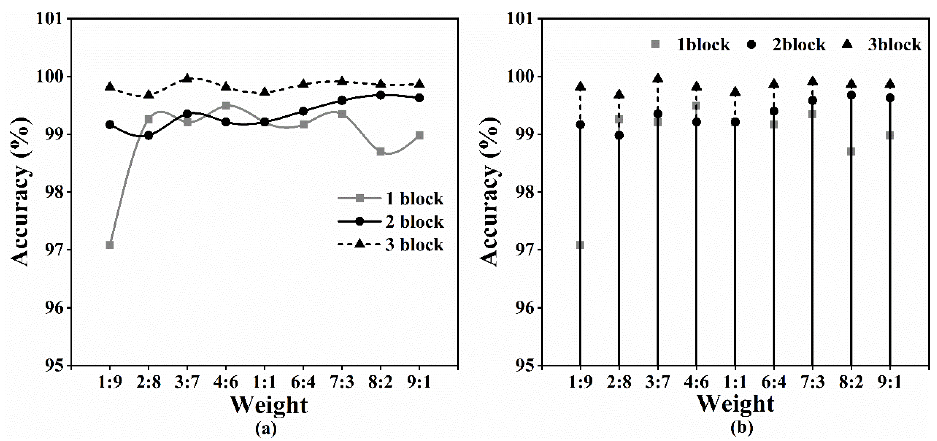
From Table 6 and Figure 14a, the highest accuracy (acc) of the single-block convolutional model under the optimal sample length of 1000 was 99.49%, and the average accuracy (acc) under different weights was 98.94%; the highest accuracy (acc) of the 2-block convolutional model was 99.68%, and the average accuracy (acc) under different weights was 99.36%; the highest accuracy (acc) of the 3-block convolutional model was 99.95%, with an average accuracy (acc) of 99.83% under different weights. Compared with the single-block convolutional model, the multi-block convolutional model had higher accuracy, faster model fitting, and better generalization ability.
The different weight ratios of multi-task also affected the model’s performance. As seen in Figure 14b, the different weight ratios of both multi-task single block and multi-block under the optimal cut-off length of 1000 affected the classification effect, reflecting the better independence and robustness of the two sub-task models.

4.6. Analysis of Multiple Evaluation Indicators of Diagnostic Results

We chose Precision, ReCall_sn, ReCall_sp, and Sacore F1, which reflect the classification of various fault types, as the evaluation metrics for the experiments to verify the performance of the model by reflecting the proportion of each type of fault being classified correctly and the level of integration. We selected the results of a multi-task single block of the multi-layer attentional convolutional model with an optimal cut length of 1000, and obtained Precision, ReCall_sn, ReCall_sp, and Sacore F1 values of the model after tri-fold cross-validation experiments on the validation set. We also took the mean values of the results of the tri-fold validation cross-validation, and looked for the minimum, maximum, and average values found from the results of 5000 rounds of experiments. From Table 7, we can see that the maximum values of Precision, ReCall_sn, ReCall_sp, and Sacore F1 of the model all reached 1, and the average values were 0.99, 0.99, 1, and 0.99, respectively, which resulted in higher values, a higher degree of equilibrium, and better diagnosis.

4.7. Comparisons with Other Works

In this section, the results of the method proposed in this paper are compared with those of the existing literature to demonstrate the advantages of the technique. The methods in the current literature are usually reached in terms of two aspects: feature extraction and fault classification. Existing methods have different fault characteristics for feature extraction and fault classification methods, and include traditional machine learning or neural networks. The comparative analysis is shown in Table 8.
It can be seen that the accuracy of the method proposed in this paper is higher than that of existing methods presented in the literature. In Ref. [33], SNN was used to encode the feature information extracted from the original vibration signal by local mean decomposition (LMD) into spike signals with an accuracy of 99.17%. In Ref. [5], A new loss function was designed and optimized with an accuracy of 96.13% using a deep self-coding method incorporating multiple fault-type discriminatory information. In Ref. [34], A multi-channel convolutional neural network (MCNN) combined with a multi-scale shear fusion (MSCF) data enhancement technique was used to achieve 99.7% classification accuracy. In Ref. [35], ESSM was used to test the performance of sparse feature extraction, sparse model construction, and its interaction mechanism with an accuracy of 96.67%. In Ref. [36], a multi-task convolutional neural network with information fusion was used to simultaneously perform both fault diagnosis and localization tasks with an accuracy of 96.04%.
The comparison results show that the method in this paper has a higher test accuracy than the multi-task CNN method and the MIMTNet method in the multi-task classification of the same CWRU dataset. It can also be seen from the different categories of fault classification that the method in this paper and the ESSM method can both do the same sample data six classification task. In contrast, the test accuracy in this paper is 3.28% higher. The results from the CWRU dataset show that the method has a high level of solid robustness and strong fault classification performance.

5. Conclusions

This paper proposes a fault diagnosis method for innovative bearings based on a multi-task deep multi-scale information fusion model (MEAT). The multi-task model performs parallel classification work to achieve accurate fault diagnosis of rolling bearings in complex practical situations. The method is validated with the vibration data from the bearing test stand of Western Reserve University. The following conclusions can be drawn from the experimental results:
(1)
The multi-task model splits the fault diagnosis six-task into a fault size dichotomous task and a fault type trichotomous task, simultaneously achieving fault-type diagnosis and size localization. The experimental results show that the model is efficient and transferable, and its robustness and generalization performance is significantly improved.
(2)
The multi-layer attention convolution model can weight and fuse bearing fault features. Compared with the standard multi-scale convolutional model and single-layer attention convolutional model, the proposed multi-layer attention convolutional model has significant advantages in fitting speed and classification accuracy.
(3)
In the multi-block model structure, each block internally extracts a broader range of complementary features through feature transfer and can obtain more abstract feature information. The experimental results show that the prediction accuracy of the multi-block model structure is significantly improved compared with that of the single-block.
(4)
To improve the interpretability of the model, we verified whether the absolute failure frequency and the model-weighted failure frequency were consistent by reverse weight exploration. The experimental results show that the model’s matching of weights and the search for fault locations were based on the original data and corresponded perfectly to the search results.
In future research, we will work on extending the proposed model to domain adaptation problems. In addition, different types of optimization algorithms can be introduced in the multi-task model to improve the overall task classification accuracy.

Author Contributions

Conceptualization, X.F.; Methodology, C.Y. and X.F.; Validation, F.M.; Formal analysis, C.Y.; Investigation, T.W.; Data curation, F.M.; Writing—original draft, R.X.; Writing—review and editing, T.W.; Project administration, R.X. All authors have read and agreed to the published version of the manuscript.

Funding

This research is supported by the Science and Technology Project of the Education Department of Jilin Province (JJKH20220245KJ, JJKH20220226SK), the National Natural Science Foundation of China Joint Fund Project (U19A200496).

Data Availability Statement

The data used in this study is a public dataset from Western Reserve University, the link to the dataset is: http://csegroups.case.edu/bearingdatacenter/pages/download-data-file, accessed on 8 December 2022. And the experimental results and code generated in the study have been uploaded.

Acknowledgments

This work is supported by the Science and Technology Project of the Education Department of Jilin Province (JJKH20220245KJ, JJKH20220226SK), the National Natural Science Foundation of China Joint Fund Project (U19A200496). In addition, we are grateful to the two anonymous reviewers for their constructive comments on this article, which enriched the experimental results.

Conflicts of Interest

The authors declare no conflict of interest.

References

  1. Zhao, M.; Kang, M.; Tang, B.; Pecht, M. Deep Residual Networks With Dynamically Weighted Wavelet Coefficients for Fault Diagnosis of Planetary Gearboxes. IEEE Trans. Ind. Electron. 2018, 65, 4290–4300. [Google Scholar] [CrossRef]
  2. Shi, H.T.; Bai, X.T. Model-based uneven loading condition monitoring of full ceramic ball bearings in starved lubrication. Mech. Syst. Signal Process. 2020, 139, 106583. [Google Scholar] [CrossRef]
  3. Li, X.; Li, J.; Zhao, C.; Qu, Y.; He, D. Gear pitting fault diagnosis with mixed operating conditions based on adaptive 1D separable convolution with residual connection. Mech. Syst. Signal Process. 2020, 142, 106740. [Google Scholar] [CrossRef]
  4. Zhang, Y.; Randall, R.B. Rolling element bearing fault diagnosis based on the combination of genetic algorithms and fast kurtogram. Mech. Syst. Signal Process. 2009, 23, 1509–1517. [Google Scholar] [CrossRef]
  5. Mao, W.; Feng, W.; Liu, Y.; Zhang, D.; Liang, X. A new deep auto-encoder method with fusing discriminant information for bearing fault diagnosis. Mech. Syst. Signal Process. 2021, 150, 107233. [Google Scholar] [CrossRef]
  6. Azamfar, M.; Singh, J.; Bravo-Imaz, I.; Lee, J. Multisensor data fusion for gearbox fault diagnosis using 2-D convolutional neural network and motor current signature analysis. Mech. Syst. Signal Process. 2020, 144, 106861. [Google Scholar]
  7. Xu, G.; Hou, D.; Qi, H.; Bo, L. High-speed train wheel set bearing fault diagnosis and prognostics: A new prognostic model based on extendable useful life. Mech. Syst. Signal Process. 2021, 146, 107050. [Google Scholar] [CrossRef]
  8. Cui, L.; Huang, J.; Zhang, F.; Chu, F. HVSRMS localization formula and localization law: Localization diagnosis of a ball bearing outer ring fault. Mech. Syst. Signal Process. 2019, 120, 608–629. [Google Scholar] [CrossRef]
  9. Zhao, X.; Jia, M. A novel unsupervised deep learning network for intelligent fault diagnosis of rotating machinery. Struct. Health Monit. 2019, 19, 1745–1763. [Google Scholar] [CrossRef]
  10. Cai, B.; Zhao, Y.; Liu, H.; Min, X. A Data-Driven Fault Diagnosis Methodology in Three-Phase Inverters for PMSM Drive Systems. IEEE Trans. Power Electron. 2017, 32, 5590–5600. [Google Scholar] [CrossRef]
  11. Ming, Z.; Jiang, Z.; Feng, K. Research on variational mode decomposition in rolling bearings fault diagnosis of the multistage centrifugal pump. Mech. Syst. Signal Process. 2017, 93, 460–493. [Google Scholar]
  12. Liu, H.; Zhang, J.; Cheng, Y.; Lu, C. Fault diagnosis of gearbox using empirical mode decomposition and multi-fractal detrended cross-correlation analysis. J. Sound Vib. 2016, 385, 350–371. [Google Scholar] [CrossRef]
  13. Zhang, G.; Wang, H.; Zhang, T.Q. Stochastic resonance of coupled time-delayed system with fluctuation of mass and frequency and its application in bearing fault diagnosis. J. Cent. South Univ. 2021, 28, 2931–2946. [Google Scholar] [CrossRef]
  14. Ma, Y.; Huang, Q.; Zhang, Z.; Cai, D. Application of Multisynchrosqueezing Transform for Subsynchronous Oscillation Detection Using PMU Data. IEEE Trans. Ind. Appl. 2021, 57, 2006–2013. [Google Scholar] [CrossRef]
  15. Wen, L.; Li, X.; Gao, L.; Zhang, Y. A New Convolutional Neural Network-Based Data-Driven Fault Diagnosis Method. IEEE Trans. Ind. Electron. 2017, 65, 5990–5998. [Google Scholar] [CrossRef]
  16. Hu, Z.X.; Wang, Y.; Ge, M.F.; Liu, J. Data-driven Fault Diagnosis Method based on Compressed Sensing and Improved Multi-scale Network. IEEE Trans. Ind. Electron. 2020, 67, 3216–3225. [Google Scholar] [CrossRef]
  17. Fuan, W.; Hongkai, J.; Haidong, S.; Wenjing, D.; Shuaipeng, W. An adaptive deep convolutional neural network for rolling bearing fault diagnosis. Meas. Sci. Technol. 2017, 28, 095005. [Google Scholar] [CrossRef]
  18. Zhang, W.; Peng, G.; Li, C.; Chen, Y.; Zhang, Z. A new deep learning model for fault diagnosis with good anti-noise and domain adaptation ability on raw vibration signals. Sensors 2017, 17, 425. [Google Scholar] [CrossRef]
  19. Zhang, D.; Zhou, T. Deep convolutional neural network using transfer learning for fault diagnosis. IEEE Access 2021, 9, 43889–43897. [Google Scholar] [CrossRef]
  20. Kumar, A.; Zhou, Y.; Gandhi, C.; Kumar, R.; Xiang, J. Bearing defect size assessment using wavelet transform based Deep Convolutional Neural Network (DCNN). Alex. Eng. J. 2020, 59, 999–1012. [Google Scholar] [CrossRef]
  21. Lecun, Y.; Bengio, Y.; Hinton, G.J.N. Deep learning. Nature 2015, 521, 436–444. [Google Scholar] [CrossRef]
  22. Hao, X.; Zhang, G.; Ma, S.J.I.J.o.S.C. Deep learning. Int. J. Semant. Comput. 2016, 10, 417–439. [Google Scholar] [CrossRef] [Green Version]
  23. Liu, W.; Wen, Y.; Yu, Z.; Yang, M. Large-Margin Softmax Loss for Convolutional Neural Networks. arXiv 2016, arXiv:1612.02295, 137–164. [Google Scholar]
  24. Li, Y.; Wang, N.; Shi, J.; Liu, J.; Hou, X. Revisiting Batch Normalization For Practical Domain Adaptation. Pattern Recognit. 2016, 80, 3203. [Google Scholar]
  25. Xu, Z.; Li, C.; Yang, Y. Fault diagnosis of rolling bearings using an Improved Multi-Scale Convolutional Neural Network with Feature Attention mechanism. ISA Trans. 2020, 110, 379–393. [Google Scholar] [CrossRef] [PubMed]
  26. Lai, T.; Cheng, L.; Wang, D.; Ye, H.; Zhang, W. RMAN: Relational multi-head attention neural network for joint extraction of entities and relations. Appl. Intell. 2021, 52, 3132–3142. [Google Scholar] [CrossRef]
  27. Hackel, T.; Usvyatsov, M.; Galliani, S.; Wegner, J.D.; Schindler, K. Inference, Learning and Attention Mechanisms that Exploit and Preserve Sparsity in Convolutional Networks. Int. J. Comput. Vis. 2020, 128, 656. [Google Scholar] [CrossRef]
  28. Wang, H.; Xu, J.; Yan, R.; Sun, C.; Chen, X. Intelligent Bearing Fault Diagnosis Using Multi-Head Attention-Based CNN. Procedia Manuf. 2020, 49, 112–118. [Google Scholar] [CrossRef]
  29. Vaswani, A.; Shazeer, N.; Parmar, N.; Uszkoreit, J.; Jones, L.; Gomez, A.N.; Kaiser, L.; Polosukhin, I. Attention is All You Need. Adv. Neural Inf. Process. Syst. 2017, 1–15. [Google Scholar]
  30. Shao, H.; Xia, M.; Han, G.; Zhang, Y.; Wan, J. Intelligent fault diagnosis of rotor-bearing system under varying working conditions with modified transfer CNN and thermal images. IEEE Trans. Ind. Inform. 2020, 17, 3488–3496. [Google Scholar] [CrossRef]
  31. Xie, Z.; Chen, J.; Feng, Y.; Zhang, K.; Zhou, Z. End to end multi-task learning with attention for multi-objective fault diagnosis under small sample. J. Manuf. Syst. 2022, 62, 301–316. [Google Scholar] [CrossRef]
  32. Keskar, N.S.; Socher, R. Improving generalization performance by switching from adam to sgd. arXiv 2017, arXiv:1712.07628. [Google Scholar]
  33. Zuo, L.; Zhang, L.; Zhang, Z.H.; Luo, X.L.; Liu, Y. A spiking neural network-based approach to bearing fault diagnosis. J. Manuf. Syst. 2021, 61, 714–724. [Google Scholar] [CrossRef]
  34. Bai, R.X.; Xu, Q.S.; Meng, Z.; Cao, L.X.; Xing, K.S.; Fan, F.J. Rolling bearing fault diagnosis based on multi-channel convolution neural network and multi-scale clipping fusion data augmentation. Measurement 2021, 184, 109885. [Google Scholar] [CrossRef]
  35. Zhang, F.; Yan, J.; Fu, P.; Wang, J.; Gao, R.X. Ensemble sparse supervised model for bearing fault diagnosis in smart manufacturing. Robot. Comput.-Integr. Manuf. 2020, 65, 101920. [Google Scholar] [CrossRef]
  36. Guo, S.; Zhang, B.; Yang, T.; Lyu, D.; Gao, W. Multitask Convolutional Neural Network With Information Fusion for Bearing Fault Diagnosis and Localization. IEEE Trans. Ind. Electron. 2020, 67, 8005–8015. [Google Scholar] [CrossRef]
  37. Wang, Y.; Yang, M.; Li, Y.; Xu, Z.; Wang, J.; Fang, X. A multi-input and multi-task convolutional neural network for fault diagnosis based on bearing vibration signal. IEEE Sens J. 2021, 21, 10946–10956. [Google Scholar] [CrossRef]
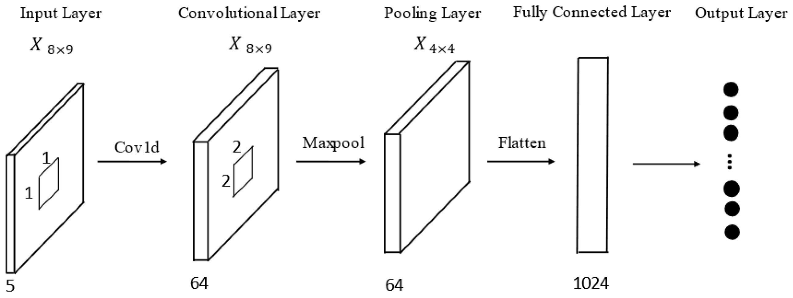
Figure 1. Typical CNN model.
Machines 11 00198 g001
Figure 2. (a) Scaled dot-product attention. (b) Multi-head attention.
Machines 11 00198 g002
Figure 3. The single-layer attention convolution model.
Machines 11 00198 g003
Figure 4. The multi-layer attention convolution model.
Machines 11 00198 g004
Figure 5. Multi-task flowchart.
Machines 11 00198 g005
Figure 6. Multiblock Learning.
Machines 11 00198 g006
Figure 7. (a) Original sequence time-domain plot; (b) frequency-domain plot.
Machines 11 00198 g007
Figure 8. Accuracy comparison between RCOV and SLAT.
Machines 11 00198 g008
Figure 9. (a) Accuracy comparison between SLAT and MLAT; (b) Comparison of rounds of SLAT and MLAT to achieve optimal results.
Machines 11 00198 g009
Figure 10. Heat map of second layer attention weighting results.
Machines 11 00198 g010
Figure 11. First layer attention weight results discounted graph.
Machines 11 00198 g011
Figure 12. (a) Original sequence time-domain plot; (b) frequency-domain plot; (c) Weighted frequency domain plot with the original sequence after taking the score; (d) Weighted frequency domain plot with the original sequence after taking the score.
Machines 11 00198 g012
Figure 13. (a) Accuracy of the STAT; (b) accuracy of the MTAT; (c) Accuracy of subtasks under optimal sample length; (d) Accuracy of subtasks with different sample lengths.
Machines 11 00198 g013aMachines 11 00198 g013b
Figure 14. (a) Accuracy comparison of Single-block models and Multi-block models; (b) Accuracy of three blocks under different weight ratios.
Machines 11 00198 g014
Table 1. Test conditions and descriptions.
Type of FaultOuter Ring FaultOuter Ring FaultInner Ring FaultInner Ring FaultBall FaultBall Fault
Fault size7 mils14 mils7 mils14 mils7 mils14 mils
NamedO 7O 14I 7I 14B_7B_14
Table 2. Experimental results of SLAT under different sample lengths.
Sample Length10020030040050060080010001200
Eval_acc (%)73.6884.0389.6293.2094.1795.3396.8596.7197.50
Train_acc (%)70.9781.6987.4791.4093.0694.2996.7097.1197.97
Best result epochs441048563425455035094922403737464860
90% of the epochs---309235204196204223
Table 3. Experimental results of MLAT under different sample lengths.
Sample Length10020030040050060080010001200
Eval_acc (%)93.4797.4398.1599.1199.0799.5399.4899.5499.67
Train_acc (%)91.9797.0997.9698.7399.0799.3599.4899.4499.72
Best result epochs499048424242471947494555479448653560
90% of the epochs205126116113152141154228252
Table 4. Accuracy of STAT and MTAT under different sample lengths.
Sample Length10020030040050060080010001200
STAT Eval_acc (%)93.4797.4398.1599.1199.0799.5399.4899.5499.67
MTAT Eval_acc (%)96.0897.0098.1399.3599.1299.4299.3799.4999.44
Table 5. Accuracy of subtasks.
Sample Length10020030040050060080010001200
Fault Type
Eval_acc (%)
94.1897.3197.8299.4398.9199.2299.0099.3199.33
Fault Size
Eval_acc (%)
96.6499.7399.8999.9899.9899.9499.9310099.94
Table 6. Experimental results under different weight ratios of a single block and multiple blocks.
Weight1:92:83:74:65:56:47:38:29:1
1 block
Eval_acc (%)
97.0899.2699.2199.4999.2199.1799.3598.798.98
2 block
Eval_acc (%)
99.1798.9899.3599.2199.2199.4099.5899.6899.63
3 block
Eval_acc (%)
99.8199.6899.9599.8199.7299.8699.9199.8699.86
Table 7. Experimental results under different evaluation indexes.
IndicatorsPrecisionReCall_snReCall_spSacore F1
Minimum value0.030.200.990.58
Maximum value1111
Average value0.990.9910.99
Table 8. Comparative analysis of CWRU dataset.
MethodsInput TypeClassesSamples LengthAccuracy (%)
SNN [33]Raw signalFault classification 412099.17
SDIAE [5]Raw signalFault classification 910096.13
MCNN [34]Raw signalFault classification 1011099.7
ESSM [35]Raw signalFault classification 630096.67
Multi-task CNN [36]Raw signalFault classification 1070096.04
MIMTNet [37]Raw signalFault Size 3
Fault Type 3
442599.96
99.22
MEAT
(Our method)
Raw signalFault Size 2
Fault Type 3
Mapping Fault classification 6
1000100
99.4
99.95
Disclaimer/Publisher’s Note: The statements, opinions and data contained in all publications are solely those of the individual author(s) and contributor(s) and not of MDPI and/or the editor(s). MDPI and/or the editor(s) disclaim responsibility for any injury to people or property resulting from any ideas, methods, instructions or products referred to in the content.