Article

On the Use of a Genetic Algorithm for Determining Ho–Cook Coefficients in Continuous Path Planning of Industrial Robotic Manipulators

1
ADRIA-ELECTRONIC Ltd., Andrije Kačića Miošića 13, 51000 Rijeka, Croatia
2
Department of Automation and Electronics, Faculty of Engineering, University of Rijeka, Vukovarska 58, 51000 Rijeka, Croatia
*
Author to whom correspondence should be addressed.
These authors contributed equally to this work.
Machines 2023, 11(2), 167; https://doi.org/10.3390/machines11020167
Submission received: 23 December 2022 / Revised: 13 January 2023 / Accepted: 22 January 2023 / Published: 25 January 2023
(This article belongs to the Special Issue Modeling, Sensor Fusion and Control Techniques in Applied Robotics)

Abstract

:
Path planning is one of the key steps in the application of industrial robotic manipulators. The process of determining trajectories can be time-intensive and mathematically complex, which raises the complexity and error proneness of this task. For these reasons, the authors tested the application of a genetic algorithm (GA) on the problem of continuous path planning based on the Ho–Cook method. The generation of trajectories was optimized with regard to the distance between individual segments. A boundary condition was set regarding the minimal values that the trajectory parameters can be set in order to avoid stationary solutions. Any distances between segments introduced by this condition were addressed with Bezier spline interpolation applied between evolved segments. The developed algorithm was shown to generate trajectories and can easily be applied for the further path planning of various robotic manipulators, which indicates great promise for the use of such algorithms.

1. Introduction

The most significant element in the application of industrial robotic manipulators on realistic tasks is the path planning process [1]. This process determines the trajectory of the joint movements—their positions, speeds, and accelerations—allowing the robotic manipulator to perform operations within its environment [2]. The goal of path planning is to calculate paths that satisfy the preset conditions that have to be fulfilled in order to accomplish the task. There are two main paradigms of trajectory determination: point-to-point and continuous path planning [3,4]. Point-to-point planning concerns itself with generating paths between two points in space and is commonly used for operations such as the pick-and-place transfer of objects [5]. Continuous path planning, on the other hand, takes into account the movement not just between the initial and final points in space but also the positions and speeds between them. Such an approach is commonly used for tasks such as welding or painting objects in space [6]. Multiple deterministic methods can be used to perform the path planning of industrial robotic manipulators continuously: Ho–Cook [7], Taylor’s polynomial approach [8], or interpolation between trajectory points [9]. While these algorithms perform well, they can be computationally complex and, depending on the mode of application, error-prone. Evolutionary computing is a branch of artificial intelligence that deals with the study of algorithms that imitate natural processes [10]. The basic algorithm in this area is the so-called genetic algorithm, which, by its design, imitates the natural process of evolution [11]. Evolutionary computing algorithms have been shown to have many uses in robotics [12].
Shukla et al. (2021) [13] demonstrated the use of evolutionary computing for robotic grasp manipulation. The authors applied EC algorithms to assist in training deep learning models, in an approach known as hybrid models. They managed to achieve high-precision models with this approach. Ferigo et al. (2021) [14] applied evolutionary computing algorithms for evolving sensory apparatus in soft computing applications. Kim et al. (2021) [15] demonstrated the application of evolutionary computing for the issue of quadruped robot gait optimization. The authors utilized GA to create paths for mobile robots’ legs to achieve a more controlled gait. Liu et al. (2022) [16] created a digital twin, which is a virtualized copy of a real robot. The authors then demonstrated the ability to apply GA for the path planning of such a robot, which they managed to successfully transfer to a real robot. Li et al. (2021) [17] addressed another important issue in robotics: task allocation through the application of a differential evolution algorithm. The authors managed to achieve state-of-the-art results on a multitask optimization problem. Task allocation was also addressed by Martin et al. (2021) [18]. In this paper, the authors specifically used GA to distribute the tasks amongst robots based on the nonlinear branching criteria. Path planning for robots was also addressed by Hao et al. (2021) [19]. The authors utilized GA to optimize a path concerning the possible collision risks, achieving paths that are capable of avoiding obstructions in the space. A similar approach was demonstrated by Rahmaniar and Rakhmania (2022) [20] for mobile robots. The authors demonstrated that GA-optimized paths are capable of achieving smoother paths when compared to classical methods. Tuning the paths based on Bezier splines can also be achieved using evolutionary computing algorithms, as demonstrated by Song et al. (2021) [21], who applied particle swarm optimization to determine the parameters of the splines. Li et al. (2022) [22] demonstrated the subgoal hybrid planning for the path smoothing of paths obtained with forward search optimization in contrast to Djikstra, A*, D*, and D*-lite algorithms. The authors compared the performance of forward search optimization and the newly developed subgoal-based hybrid path planning algorithm, demonstrating that smooth global paths can be achieved with such an approach. A similar approach to the one presented in this paper, where a deterministic algorithm A* is combined with an evolutionary approach, namely the coevolutionary algorithm, was adapted by Garcia et al. (2023) [23]. The authors demonstrated that such an approach has a high enough performance for applications on edge nodes, and performs well in conditions where alternatives such as M* or WHCA would fail to generate valid paths. Yu et al. (2023) [24] applied the artificial bee colony to optimize a multi-objective path planning issue. The authors demonstrated that such an algorithm can be successfully applied to multi-objective problems, namely path efficiency and path security. Another nature-inspired algorithm was shown by Wu et al. [25], who applied the ant colony algorithm to the path planning of the mobile robot. The modified version of the ant colony algorithm that the authors developed shows a significant improvement in comparison to the state-of-the-art methods. Lou et al. (2023) [26] applied a graphical computing method for the problem of continuous path planning for welding. The simulations performed by the authors on the generated paths demonstrate the possibility of applying the investigated method in real-word applications. Another industrial production application, namely surface grinding, was discussed by Li et al. (2023) [27]. The authors applied a revised Levenberg–Marquardt and differential evolution hybrid algorithm, with real-world validation on the problem of grinding titanium blades.
While the state-of-the-art research shows many applications of evolutionary computing and GA in the area of robotics and path planning, none address the combination of algorithms such as Ho–Cook with GA or similar evolutionary algorithms.
The Ho–Cook algorithm was selected in particular as the topic of the research due to several advantages that it possesses compared to similar algorithms: mainly the ability to manually select as many points as desired (allowing for the granular control of the trajectory precision) and the fact that it includes the orientation of the tool, by design—as will be shown in Section 2. Due to the lack of previous research focusing on the Ho–Cook algorithm parameter tuning with evolutionary algorithms, the authors selected GA as the second focus of the research. GA is the basic evolutionary algorithm, which means that it should serve as a good indicator of performance for more advanced algorithms [28,29]. The gene setup that was developed and is presented in Section 2.2 of this manuscript is also novel, and customized to the Ho–Cook problem. This chromosome encoding describes the Ho–Cook parametrization and may be used as the basis for the further research of additional, more advanced evolutionary algorithms, as most algorithms of this kind will require this encoding to be performed in the same manner [12,30].
The goal of this paper was to test whether the process of path planning in a continuous environment, based on the Ho–Cook algorithm, can be simplified through the application of the GA. In addition, the parameters of GA that provide the best performance were also determined. In this approach, the common issues in continuous path planning are addressed through the Ho–Cook algorithm, whose shortcoming is the analytical complexity of the coefficient determination, as will be shown in Section 2.

2. Materials and Methods

This section will serve to present the basic idea of the Ho–Cook path planning process to point out which part of it will be tuned using the GA-based approach. Then, the process of GA development will be described.

2.1. Ho–Cook Path Planning

The Ho–Cook path planning algorithm is a continuous path planning algorithm. It is based on determining n points that will be the elements of the trajectory. In the case of the obstacles being present in the tool space inside of which the path planning is being performed, the aforementioned points should be placed in such a way that obstacles are not present, as obstacle avoidance is not a built-in feature of the Ho–Cook method [31]. Due to the Ho–Cook method having to pass through the points defined initially, as they are starting/ending points of the segments, the movement from the source to the destination is guaranteed. The Ho–Cook method works by interpolating between the aforementioned points of the desired trajectory to achieve the shortest possible path through the calculation of in-between segments. Higher-order polynomials (4th and 3rd) are used to assure the smoothness of the final trajectory. Then, the n 1 segments between the points are interpolated using the polynomials given as [32]:
q k ( t ) = B 0 k + B 1 k t + B 2 k t 2 + B 3 k t 3 + B 4 k t 4
for the first and the last segments, whereas the other segments are interpolated using:
q k ( t ) = B 0 k + B 1 k t + B 2 k t 2 + + B 3 k t 3
The speeds and accelerations can be derived from the above. For the first and the last segment, they are given as:
q k ( t ) ˙ = B 1 k + 2 B 2 k t + 3 B 3 k t 2 + 4 B 4 k t 3 ,
and
q k t ¨ = 2 B 2 k + 6 B 1 k t + 12 B 4 k t 2
respectively. The speed and acceleration for the other segments are given similarly with:
q k ( t ) ˙ = B 1 k + 2 B 2 k t + 3 B 3 k t 2 ,
and
q k t ¨ = 2 B 2 k + 6 B 1 k t + 12 B 4 k t 2 .
In the above equations, the symbols used are as follows:
  • k—the trajectory point;
  • m—the total number of trajectory points, and
  • B—coefficients of the interpolation polynomials.
For each of the segments, a number of coefficients need to be determined. They can be defined within the matrix of the shape k × n , where n is the polynomial degree (third or fourth) and k is the number of the joints of the robotic manipulator. In the presented research, the number of joints was assumed to be six, since this is a common number of degrees of freedom for industry-standard articulated robots [33].
To determine the above, the Dennavit–Hartenberg (D-H) algorithm was performed. First, the simplified kinematic schematic with the noted rotation axes was designed for the robot that is being modeled. An example of the ABB IRB 120 robot can be seen in Figure 1. On the schematic, the joints of the robot have orthonormal coordinate systems adjoined, with the orientation dependent on the rotation axes of the robot in question [34].
This will allow us to determine the kinematic properties of the robot, which can be read from the schematic: joint distance d, joint angle θ , link length a, and link rotation angle α [35]. The obtained kinematics properties for the robot in question are given in Table 1.
The next step is to obtain the kinematic transformation matrix, T 0 6 , which is the product of each individual joint transformation matrix [35]:
T 0 6 = Π k = 1 6 c o s θ k c o s α k s i n θ k s i n α k s i n θ k a k c o s θ k s i n θ k c o s α k c o s θ k s i n α k cos θ k a k s i n θ k 0 s i n α k c o s α k d k 0 0 0 1
Inserting the values from Table 1 into the above equation yields the following equation that describes the transformation matrix:
T 0 6 = [ [ 1.0 ( ( s i n ( q 1 ) s i n ( q 4 ) + c o s ( q 1 ) c o s ( q 4 ) c o s ( q 2 + q 3 ) ) c o s ( q 5 ) s i n ( q 5 ) s i n ( q 2 + q 3 ) c o s ( q 1 ) ) c o s ( q 6 ) + 1.0 ( s i n ( q 1 ) c o s ( q 4 ) 1.0 s i n ( q 4 ) c o s ( q 1 ) c o s ( q 2 + q 3 ) ) s i n ( q 6 ) , 1.0 ( ( s i n ( q 1 ) s i n ( q 4 ) + c o s ( q 1 ) c o s ( q 4 ) c o s ( q 2 + q 3 ) ) c o s ( q 5 ) + s i n ( q 5 ) s i n ( q 2 + q 3 ) c o s ( q 1 ) ) s i n ( q 6 ) + 1.0 ( s i n ( q 1 ) c o s ( q 4 ) 1.0 s i n ( q 4 ) c o s ( q 1 ) c o s ( q 2 + q 3 ) ) c o s ( q 6 ) , 1.0 ( s i n ( q 1 ) s i n ( q 4 ) + c o s ( q 1 ) c o s ( q 4 ) c o s ( q 2 + q 3 ) ) s i n ( q 5 ) 1.0 s i n ( q 2 + q 3 ) c o s ( q 1 ) c o s ( q 5 ) , 0.072 s i n ( q 1 ) s i n ( q 4 ) s i n ( q 5 ) 0.072 s i n ( q 5 ) c o s ( q 1 ) c o s ( q 4 ) c o s ( q 2 + q 3 ) 0.072 s i n ( q 2 + q 3 ) c o s ( q 1 ) c o s ( q 5 ) 0.302 s i n ( q 2 + q 3 ) c o s ( q 1 ) + 0.29 c o s ( q 1 ) c o s ( q 2 ) + 0.07 c o s ( q 1 ) c o s ( q 2 + q 3 ) ] , [ 1.0 ( ( s i n ( q 1 ) c o s ( q 4 ) c o s ( q 2 + q 3 ) s i n ( q 4 ) c o s ( q 1 ) ) c o s ( q 5 ) s i n ( q 1 ) s i n ( q 5 ) s i n ( q 2 + q 3 ) ) c o s ( q 6 ) 1.0 ( s i n ( q 1 ) s i n ( q 4 ) c o s ( q 2 + q 3 ) + c o s ( q 1 ) c o s ( q 4 ) ) s i n ( q 6 ) , 1.0 ( ( s i n ( q 1 ) c o s ( q 4 ) c o s ( q 2 + q 3 ) + s i n ( q 4 ) c o s ( q 1 ) ) c o s ( q 5 ) + s i n ( q 1 ) s i n ( q 5 ) s i n ( q 2 + q 3 ) ) s i n ( q 6 ) 1.0 ( s i n ( q 1 ) s i n ( q 4 ) c o s ( q 2 + q 3 ) + c o s ( q 1 ) c o s ( q 4 ) ) c o s ( q 6 ) , 1.0 ( s i n ( q 1 ) c o s ( q 4 ) c o s ( q 2 + q 3 ) + s i n ( q 4 ) c o s ( q 1 ) ) s i n ( q 5 ) 1.0 s i n ( q 1 ) s i n ( q 2 + q 3 ) c o s ( q 5 ) , 0.072 s i n ( q 1 ) s i n ( q 5 ) c o s ( q 4 ) c o s ( q 2 + q 3 ) 0.072 s i n ( q 1 ) s i n ( q 2 + q 3 ) c o s ( q 5 ) 0.302 s i n ( q 1 ) s i n ( q 2 + q 3 ) + 0.29 s i n ( q 1 ) c o s ( q 2 ) + 0.07 s i n ( q 1 ) c o s ( q 2 + q 3 ) + 0.072 s i n ( q 4 ) s i n ( q 5 ) c o s ( q 1 ) ] , [ 1.0 ( s i n ( q 5 ) c o s ( q 2 + q 3 ) + s i n ( q 2 + q 3 ) c o s ( q 4 ) c o s ( q 5 ) ) c o s ( q 6 ) + 1.0 s i n ( q 4 ) s i n ( q 6 ) s i n ( q 2 + q 3 ) , 1.0 ( s i n ( q 5 ) c o s ( q 2 + q 3 ) + s i n ( q 2 + q 3 ) c o s ( q 4 ) c o s ( q 5 ) ) s i n ( q 6 ) + 1.0 s i n ( q 4 ) s i n ( q 2 + q 3 ) c o s ( q 6 ) , 1.0 s i n ( q 5 ) s i n ( q 2 + q 3 ) c o s ( q 4 ) 1.0 c o s ( q 5 ) c o s ( q 2 + q 3 ) , 0.29 s i n ( q 2 ) + 0.072 s i n ( q 5 ) s i n ( q 2 + q 3 ) c o s ( q 4 ) 0.07 s i n ( q 2 + q 3 ) 0.072 c o s ( q 5 ) c o s ( q 2 + q 3 ) 0.302 c o s ( q 2 + q 3 ) + 0.29 ] , [ 0 , 0 , 0 , 1 ] ]
The above matrix defines the equations that may be used to calculate the position [ x y z ] and orientation [ ϕ θ ψ ] . These equations are given as:
x = 0.072 · s i n ( q 1 ) · s i n ( q 4 ) · s i n ( q 5 ) 0.072 · s i n ( q 5 ) · c o s ( q 1 ) · c o s ( q 4 ) · c o s ( q 2 + q 3 ) 0.072 · s i n ( q 2 + q 3 ) · c o s ( q 1 ) · c o s ( q 5 ) 0.302 · s i n ( q 2 + q 3 ) · c o s ( q 1 ) + 0.29 · c o s ( q 1 ) · c o s ( q 2 ) + 0.07 · c o s ( q 1 ) · c o s ( q 2 + q 3 ) ,
y = 0.072 · s i n ( q 1 ) · s i n ( q 5 ) · c o s ( q 4 ) · c o s ( q 2 + q 3 ) 0.072 · s i n ( q 1 ) · s i n ( q 2 + q 3 ) · c o s ( q 5 ) 0.302 · s i n ( q 1 ) · s i n ( q 2 + q 3 ) + 0.29 · s i n ( q 1 ) · c o s ( q 2 ) + 0.07 · s i n ( q 1 ) · c o s ( q 2 + q 3 ) + 0.072 · s i n ( q 4 ) · s i n ( q 5 ) · c o s ( q 1 ) ,
z = 0.29 · s i n ( q 2 ) + 0.072 · s i n ( q 5 ) · s i n ( q 2 + q 3 ) · c o s ( q 4 ) 0.07 · s i n ( q 2 + q 3 ) 0.072 · c o s ( q 5 ) · c o s ( q 2 + q 3 ) 0.302 · c o s ( q 2 + q 3 ) + 0.29 ,
for the linear coordinates in the tool space, whereas the orientation is defined by:
ϕ = 1.0 · ( s i n ( q 1 ) · s i n ( q 4 ) + c o s ( q 1 ) · c o s ( q 4 ) · c o s ( q 2 + q 3 ) ) · s i n ( q 5 ) 1.0 · s i n ( q 2 + q 3 ) · c o s ( q 1 ) · c o s ( q 5 ) ,
θ = 1.0 · ( s i n ( q 1 ) · c o s ( q 4 ) · c o s ( q 2 + q 3 ) + s i n ( q 4 ) · c o s ( q 1 ) ) · s i n ( q 5 ) 1.0 · s i n ( q 1 ) · s i n ( q 2 + q 3 ) · c o s ( q 5 ) ,
and
ψ = 0.072 · s i n ( q 1 ) · s i n ( q 5 ) · c o s ( q 4 ) · c o s ( q 2 + q 3 ) 0.072 · s i n ( q 1 ) · s i n ( q 2 + q 3 ) · c o s ( q 5 ) 0.302 · s i n ( q 1 ) · s i n ( q 2 + q 3 ) + 0.29 · s i n ( q 1 ) · c o s ( q 2 ) + 0.07 · s i n ( q 1 ) · c o s ( q 2 + q 3 ) + 0.072 · s i n ( q 4 ) · s i n ( q 5 ) · c o s ( q 1 )
The above equations can be transformed in order to obtain the joint values for the given position and orientation. This is how the Ho–Cook trajectory planning process is capable of taking into account the orientation and the position, as the points that are defined as the points of the trajectory involve orientation as well as the position [ x y z ϕ θ ψ ] [31]. The process of defining the Ho–Cook trajectory can then be followed by defining the following relation:
q 2 ˙ q 3 ˙ q m 2 ˙ q m 1 ˙ 3 t 2 + 2 t 3 t 4 0 0 0 1 t 3 2 · ( t 3 + t 4 ) t 5 0 0 0 t 3 2 · ( t 4 + t 5 ) 0 0 0 0 0 t m 1 0 0 0 0 2 · ( t m 2 + t m 1 ) t t m 1 0 0 0 t m 2 2 t m 1 + 3 t m = 6 t 2 ( q 2 q 1 ) + 3 t 3 2 ( q 3 q 2 ) 3 t 3 t 4 [ t 3 2 ( q 4 q 3 ) + t 4 2 ( q 3 q 2 ) ] 3 t 4 t 5 [ t 4 2 ( q 5 q 4 ) + t 5 2 ( q 4 q 3 ) ] 6 t m 2 t m 1 [ t m 2 2 ( q m 1 q m 2 ) + t m 1 2 ( q m 2 q m 3 ) ] 6 t m 2 ( q m q m 1 ) + 3 t m 1 2 ( q m 1 q m 2 )
Finally, the segment coefficients of the Ho–Cook trajectories are then calculated using three different equation sets. The first segment coefficients are calculated as:
[ B 1 0 B 1 1 B 1 2 B 1 3 B 1 4 ] = [ q 1 q 2 q 1 ˙ q 2 ˙ ] · 1 0 0 4 t 2 3 3 t 2 4 0 0 0 4 t 2 3 3 t 2 4 0 0 0 0 0 0 0 0 1 t 2 2 1 t 2 3 .
The segments between the first and the last one can be calculated using:
[ B k 0 B k 1 B k 2 B k 3 ] = [ q k q k + 1 q k ˙ q k + 1 ˙ ] · 1 0 3 t k + 1 2 2 t k + 1 3 0 0 3 t k + 1 2 2 t k + 1 3 0 1 2 t k + 1 1 t k + 1 2 0 0 1 t k + 1 1 t k + 1 2 .
The final segment of the interpolated trajectory can then be defined as:
[ B m 1 0 B m 1 1 B m 1 2 B m 1 3 B m 1 4 ] = [ q m 1 q m q m 1 ˙ q m ˙ ] · 1 0 6 t m 2 8 t m 3 3 t m 4 0 0 6 t m 2 8 t m 3 3 t m 4 0 0 3 t 2 3 t 2 2 1 t 2 3 0 0 0 0 0
These equations also allow for the calculation of the joint positions and speeds if the coefficients are known, which will be the focus of the paper going forward. The motion of the robot is only limited by the natural limitations of the robotic manipulator at hand (for ABB IRB 120, first joint in range <−2.88, 2.88> [rad], second joint <−1.92, 1.92> [rad] third joint <−1.22, 1.92> [rad], fourth joint <−2.79, 2.79> [rad], fifth joint <−2.09, 2.09> [rad], and <0, 6.28> [rad] for the final joint) [36], or other robot positional issues, such as singularities [37]. These issues can be addressed within the GA by artificially lowering the fitness of the solutions that are outside of the bonds.

2.2. Genetic Algorithm

A genetic algorithm (GA) is an optimization algorithm based on the natural evolution process [38]. The algorithm works by generating a population of randomly selected potential solutions [28]. Then, each of these solutions is evaluated individually according to a pre-defined function: the so-called fitness function [39]. The iterating process of the GA then starts by randomly selecting the potential solutions and performing the evolutionary operations on them, which generates a new solution set [40]. This process will repeat until a satisfactory solution is achieved [16]. The process is based on the evolutionary operations, of which, there are three in GA: crossover, mutation, and reproduction. Crossover was performed on two of the randomly selected potential solutions, and they were combined into a new solution [41]. This process allows for the newly generated solutions, and when the initial random selection process is performed by weighting it towards the better-performing solutions, previous research shows that newly generated solutions tend toward the optimal solution [42]. Still, there are two issues that the crossover operation can introduce: the convergence into local optima, and the loss of quality solutions [28]. The first one was addressed by introducing the mutation operation, which will randomly modify a single randomly selected solution. This allows us to check a wider area within the possible solutions [43]. The loss of quality solutions refers to the phenomena in which a good solution is, through the application of crossover and mutation, replaced with a worse one. To address this, the reproduction operation simply transferred a quality solution into the next solution set [44]. From the above, it can be concluded that multiple values need to be defined or tested to define how the GA will be applied:
  • Shape of the potential solutions;
  • The way in which the crossover and mutation will be applied;
  • The probabilities with which the evolutionary operations will occur;
  • The fitness function that will evaluate the solutions;
  • The number of iterations (generations) of the algorithm;
  • The number of candidate solutions in the algorithm;
  • The manner of the solution selection for the operations.
Each of these elements, in the context of the paper’s goal, will be further discussed.

2.2.1. Solution Construction

The shape of the individual solutions first needs to be determined, as it is the basis for defining the remaining elements of GA. In the discussed problem, it was decided that a six-point trajectory would be used; in other words, five segments need to be generated in the shape of the vectors B 1 , B 2 , B 3 , B 4 , B 5 . According to the previous subsection, B 1 and B 5 consist of five elements and the remaining ones consist of four elements. For simplicity, all of these elements were joined in a single vector that can be used for the evolutionary computation operations as:
B = [ B 1 0 B 1 1 B 1 2 B 1 3 B 1 4 B 2 0 B 2 1 B 2 2 B 2 3 B 3 0 B 3 1 B 3 2 B 3 3 B 4 0 B 4 1 B 4 2 B 4 3 B 5 0 B 5 1 B 5 2 B 5 3 B 5 4 ] .
Each of the initial population candidate solutions were uniformly randomly filled with values in the range of [ 5 , 5 ] . Trajectory points were set randomly.

2.2.2. Application of Evolutionary Computing Operations

The three aforementioned operations—crossover, mutation, and reproduction—need to be defined, as their manner of implementation is an important element. Each of the operations also has a probability of occurring, with the previous research in the area indicating that the probability of the crossover occurring should be very high (>80%), whereas the mutation should be low (<5%), with the remaining iterations being fulfilled with the reproduction [45]. Reproduction is the simplest, as it only copies the potential solution between the generations. Its occurrence was set to 7%. The manner in which the crossover was implemented was the so-called random crossover. As shown in Equation (19), each of the segments has an individual set. The algorithm of crossover was then performed on two candidate solutions. For each of the five segments, one of the two candidate solutions was selected, and its segment was inserted into the new solution. This process is shown in Figure 2. This yields a solution that is the combination of segments from previous solutions.
The crossover operation was performed with the 90 % probability. Finally, the mutation needs to be performed. The mutation will randomly replace an entire segment of the randomly selected solution, as shown in Figure 3. Without this mechanic, due to how the crossover operation is performed, only the initially generated segments are present in all of the generations of the algorithm. The occurrence rate of this operation was set to 3 % .

2.2.3. The Fitness Function

To determine the quality of the solution, a fitness function needs to be determined. Such a function should be simple to calculate to allow for a fast calculation and execution of the algorithm while providing a realistic metric of the agent performance [46]. As can be seen in the previous Figure 2 and Figure 3, the segments generated by the GA are not continuous with each other. This is one of the main points that need to be addressed when trajectory planning is performed, and, as such, this was selected to represent the measure of quality for the candidate solution. An illustration of these distances is given in Figure 4.
To calculate this, the sum of all of the vertical distances between the segments was considered and calculated. In other words, if the last value of segment B k is given as B k [ i ] and the first value of the following segment B k + 1 is given as B k + 1 [ 0 ] , the fitness function F can be defined as:
F = k = 0 4 | B k [ i ] B k + 1 [ 0 ] | .
Due to this being a minimization problem, the lower value of the fitness function indicates a higher-quality solution. It is important to note that boundary conditions need to be set. The initial testing showed that, when allowing the GA to minimize the distance completely, solutions will tend to a stationary trajectory, without any movement amongst the segments. In other words, the elements of the matrix given in Equation (19) will converge to zero. As this is not the desired outcome, the boundary condition was introduced. The boundary condition stated defines that all candidate solutions must have a total sum of the trajectory parameters equal to or higher than a certain value, which will be determined through testing. All of the candidate solutions that do not satisfy this condition will be removed from the population, and replaced with another randomly generated solution that does satisfy the aforementioned condition.

2.2.4. Candidate Solution Selection

To achieve an improvement across the generations of the GA, the candidate solutions selected for the application of evolutionary operations need to be selected wisely. Only if the solutions selected are of high quality can the improvement in the overall population fitness be expected. To achieve this, a fitness proportionate selection was used. This refers to the type of randomized selection in which fitness is of a higher quality. The type of fitness proportional selection used in the presented work was the so-called roulette wheel selection. In this type of selection, the probability of selecting a certain candidate solution is equal to its ratio to the overall fitness. If the total fitness is F t o t a l and the individual fitness of candidate solution A is F A , then the probability of selecting it would be equal to:
p A = F A F t o t a l .
Since, in the presented case, the smaller fitness indicates the better solution, the above method can be applied to calculating a vector that determines the probability of each candidate solution, sorted in descending order. The candidate solution’s probabilities are then sorted in reverse order and the individual probability is assigned to each. This process is illustrated in Figure 5.
With all of these elements defined, it can be stated that the GA used in this research is the GA based on crossover and mutation with the roulette-wheel type selection and fixed fitness function [47].

2.3. Interpolation

Previously, when discussing the fitness value used during the presented research, it was mentioned that the lower bound needed to be set on the fitness that the solutions can achieve in order to prevent the stationary solutions. This approach yields solutions that will, even when optimized fully to the extent of the GA possibility, have vertical gaps between segments, meaning that a trajectory generated in such a manner cannot be considered as continuous. To address this, an interpolation technique was introduced. As the length of each segment is defined as 1 [s], the starting and ending 0.1 [s] of each segment were deleted. The first and final segments only had their final or initial 0.1 [s] element removed, respectively. This yields four missing segments, with a length of 0.2 s that need to be interpolated.
Interpolation was performed using second-degree Bezier splines [48], defined as [49]:
B i , k ( x ) = x t i t i + k t i B i , k 1 ( x ) + t i + k + 1 x t i + k + 1 t i + 1 B i + 1 , k 1 ( x ) ,
and
B i , 0 ( x ) = 1 , x [ t i , t i + 1 > 0 , o t h e r w i s e .
In the equations, t is the number of Bezier spline nodes, c is the coefficient of the spline determined based on the values of segments being connected, and k is the spline degree, equal to 2. An example of the result concerning the spline is given in the following section.

3. Results and Discussion

In this section, the results of the applied methodology will be discussed. The results in the process determination of boundary conditions for the obtained matrices will be demonstrated and commented on, followed by the results of GA parameter testing.

3.1. Determining the Optimal Boundary Condition

As mentioned previously, the boundary conditions were set as the minimal value of the sum of all elements of the candidate solution vector as given in Equation (19). Five different values of the bound were tested: no boundary conditions, 0.2, 0.1, 0.05, and 0.005. For the testing of the bound, the population size of the candidate solutions and the number of generations were both set to 10. While these parameter values are too small to achieve any significant results, as shown by further testing, they perform well enough to indicate the performance of the boundary condition tested without requiring too much execution time. For each of the tests performed, the results will be given as a visualization of the best-performing candidate solution at the end of the optimization process (joint positions, speeds, and accelerations given), along with a graph showing the change in the fitness of the best solution through the optimization process.
The first test was performed without any boundary condition set, and the results are shown in Figure 6. As can be seen, there are minimal movements of the robotic manipulator present, with the joint movement ranging from 0.1 to −0.25.
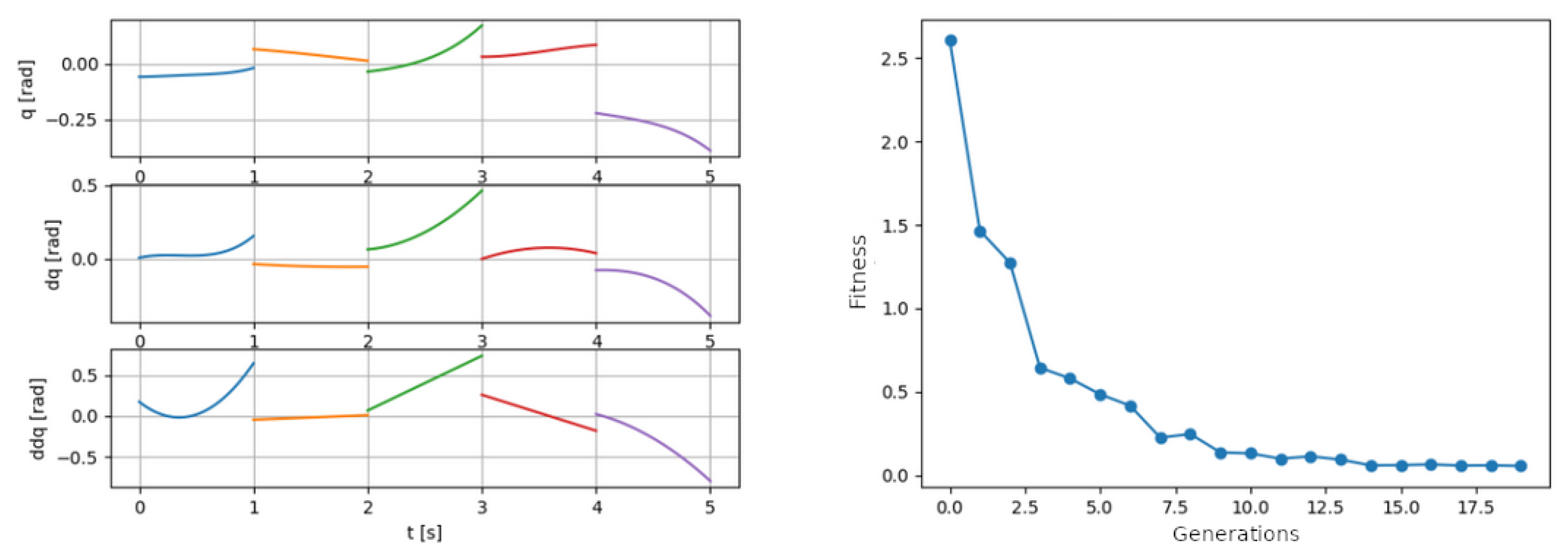
The first introduced boundary condition has a value of 0.2 and the results are shown in Figure 7. Here, it can be seen that the range of movement is higher, but, observing the graph of fitness through generations, we can see that the value to which the algorithm converges is very high.
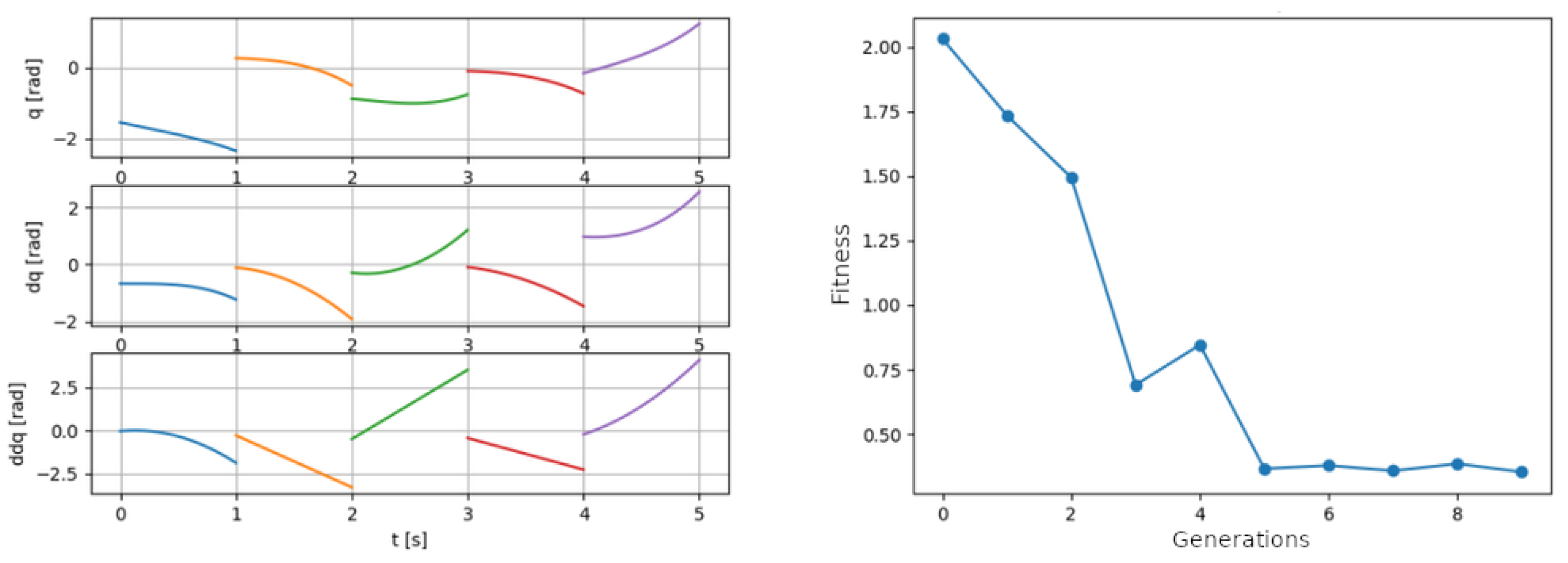
Similar but slightly improved results are achieved with the bound set to 0.1, seen in Figure 8. The range of the movement is kept, but the algorithm converges to a better overall solution. The improved results achieved by setting this value indicate the need to continue testing lower values.
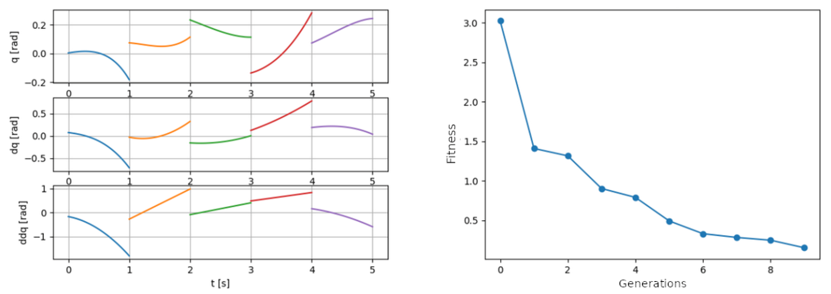
When the boundary condition is set to the value of 0.05, the graphs given in Figure 9 indicate that the movement range is kept with a further improvement in the convergence value of optimization, with the distances between segments below 0.05 [rad] and the range of motion above 1.0 [rad].
The final value for the boundary condition tested was 0.005, as demonstrated in Figure 10. This value shows a similar behavior to the configuration in which no boundary condition is set. This indicates that values this low should not be considered.
The tests performed indicate that lowering the boundary condition improves the results of the GA, as long as the condition is not set too low. When the condition is set too low, the GA performs in the same manner as it does when no condition is set. For this reason, the boundary condition of 0.05 was selected for further testing.

3.2. Determining the GA Parameters

After the boundary condition was determined and set to 0.05, the main parameters of the GA—the population size and the number of generations that the algorithm will run for—needed to be determined. Three separate configurations were tested:
  • Population size of 100 executed for 100 generations;
  • Population size of 1000 executed for 50 generations;
  • Population size of 10,000 executed for 20 generations.
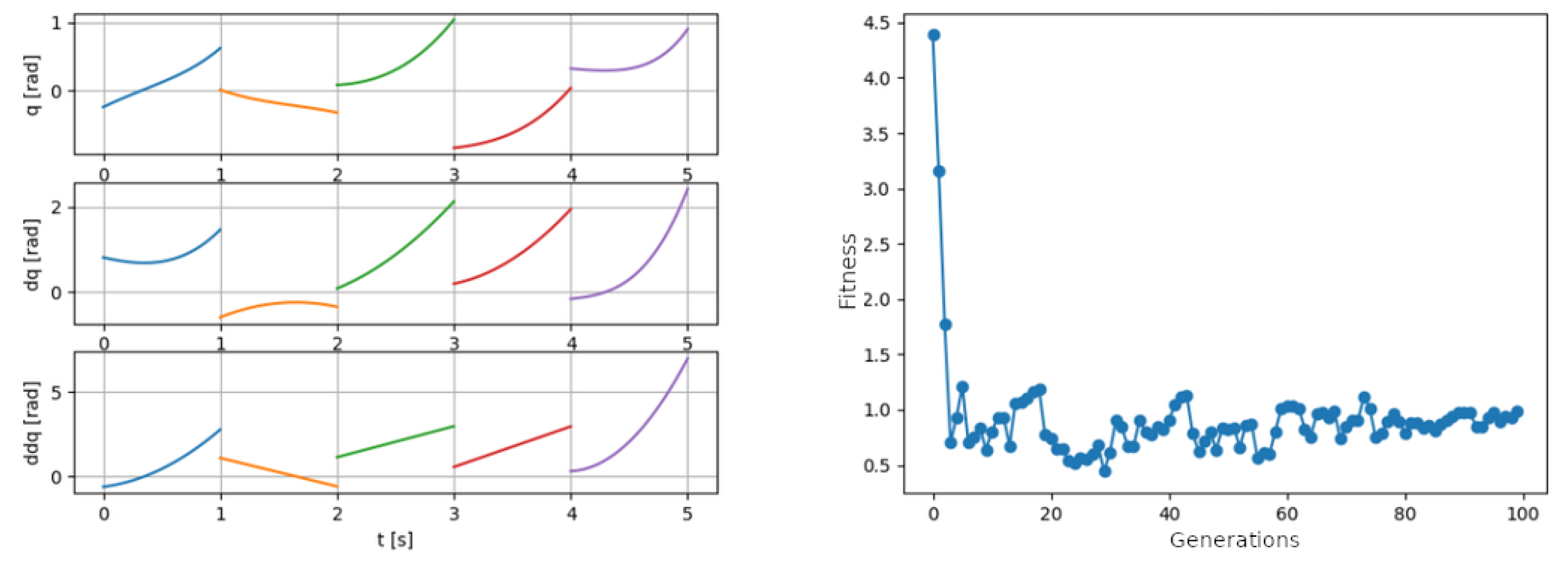
The first configuration, with 100 candidate solutions and 100 generations, is the least memory-intensive and computationally complex due to the fact that it has the lowest population value. It is shown to achieve a fitness function of 1.001, which is not satisfactory in the context of the problem. The achieved solution shows the large distances between multiple sections of the trajectory. The results are presented in Figure 11.
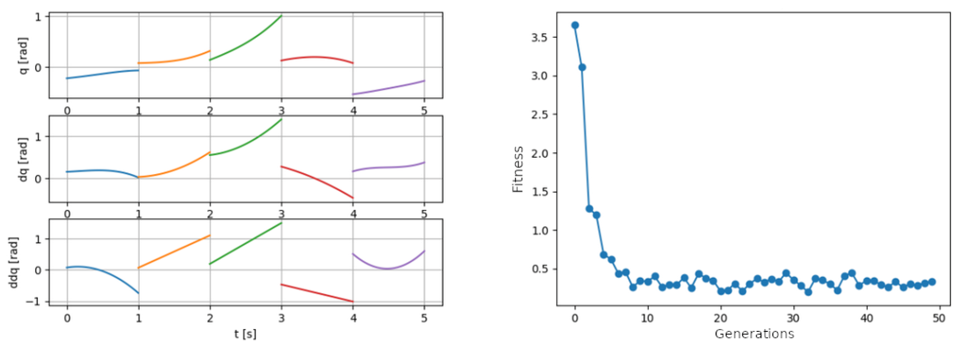
An increase in the population size to 1000 yields a significant increase in performance, even with the lower generation bound of 50. As shown in Figure 12, the lower number of generations does not negatively affect the performance, as the algorithm is shown to converge significantly before the fiftieth generation. The lowest achieved fitness function value is 0.33, which may be considered satisfactory.
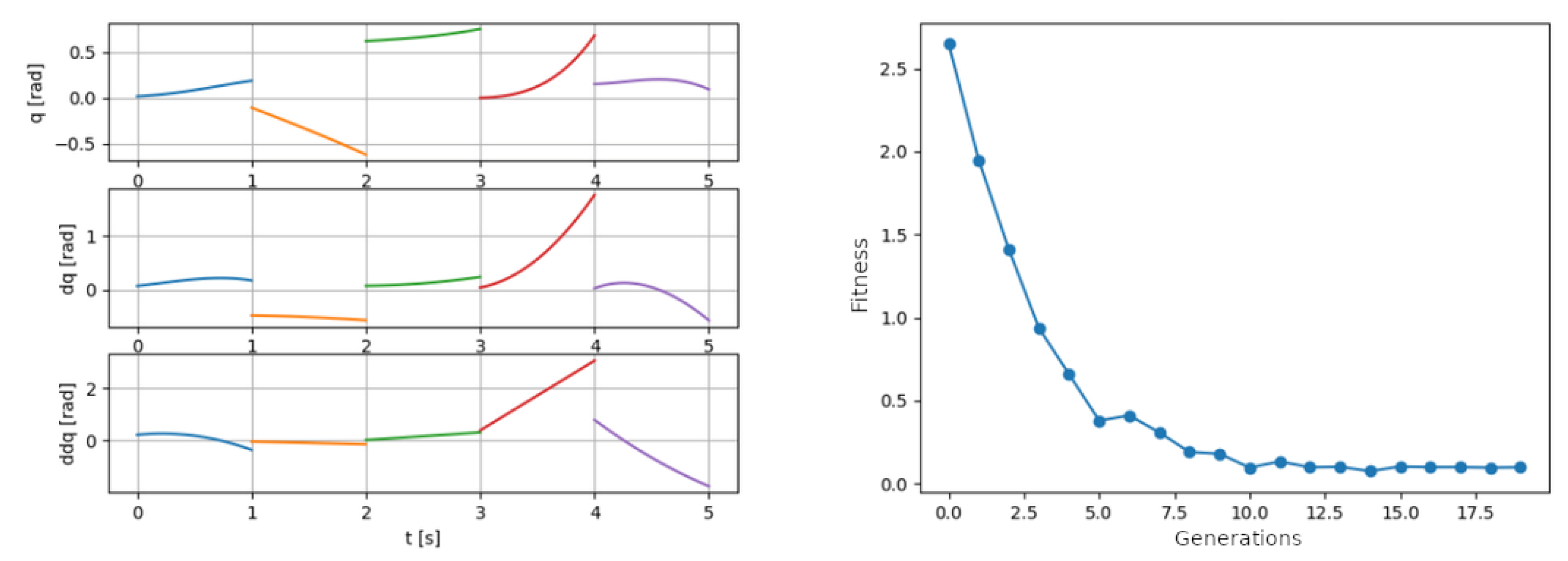
The final tested configuration has 10,000 candidate solutions and was optimized for 20 generations, the results of which are shown in Figure 13. The trend from the previous configuration continues, as the larger configuration achieves a significantly improved result of 0.098. The GA converges between generations 12 and 15, indicating that 20 generations selected for this algorithm are enough for it to converge, despite the larger population size.
To discuss the overall results, it is shown that an increase in population size yields significant performance increases. The number of generations seems to have less of an influence, and can be more limited in further research, as the algorithm tends to converge to a solution around the 15th generation in all of the tested cases.

Execution Time

An important consideration for the application of algorithms is the execution times of the algorithms in tested configurations. The tests were performed on all the previously tested configurations and averaged across 10 runs. The configuration used for testing was a laptop computer with CPU Intel(R) Core(TM) i7-1065G7 CPU, with the CPU clock locked at 1.30 GHz for the test. The machine was equipped with 16 GB of RAM. The code was executed in a single-threaded mode. The results of the test are given in Table 2.
It can be seen that the average time per each agent in the population remains relatively uniform (around 2 · 10 3 s). This means that the increase in population size has a significant influence on execution times. The smallest configuration, which yields the poorest results, finishes the execution in around twenty seconds. The two following configurations take almost two minutes, or slightly below seven minutes, respectively.

3.3. Result Illustration

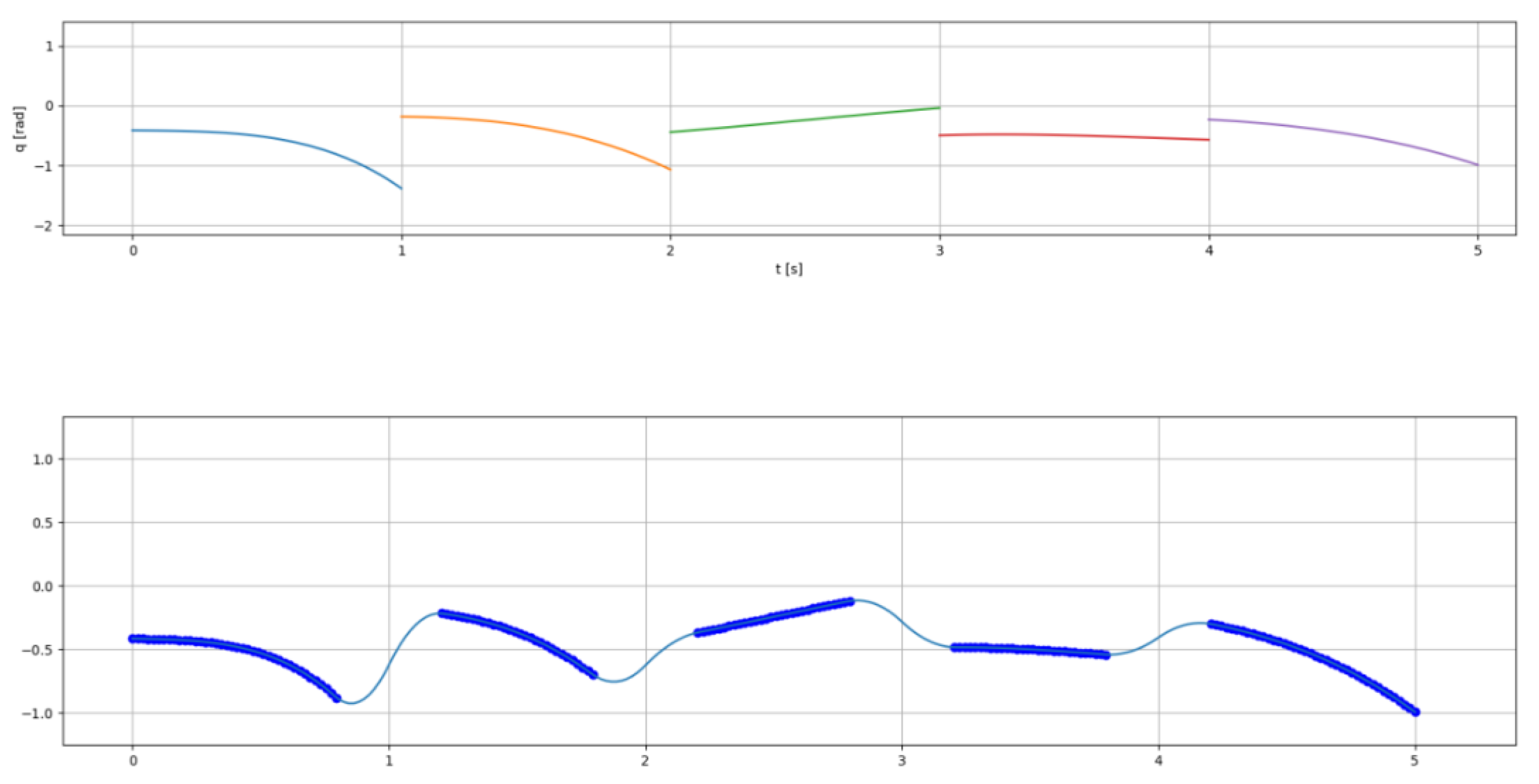
The path as given in the Figure 14 represents the motion of the joint over the course of five seconds between the position of −0.47 [rad] to 1.0 [rad]. The generated path is smooth, without any sudden changes in the joint motion direction, owing to the interpolation accomplished with Bezier splines. Some minor changes to the torque and negative vibrations may be present due to the changes in the direction present between the points, but as these transitions are smooth, these effects should not be overly negative on the motion of the path. The motion not being monotonous may have a negative effect in the sense of using more energy than would be necessary if manually tuned coefficients were used, but this negative effect should be minor and outweighed by the complexity of manually tuning the parameters, except in situations where lowering the energy use is crucial. The motion is continuous through the path, without discrete points of the Ho–Cook method being clearly visible. Any delays in the movement should not be present with the generated path, as the entire generated trajectory is continuous.
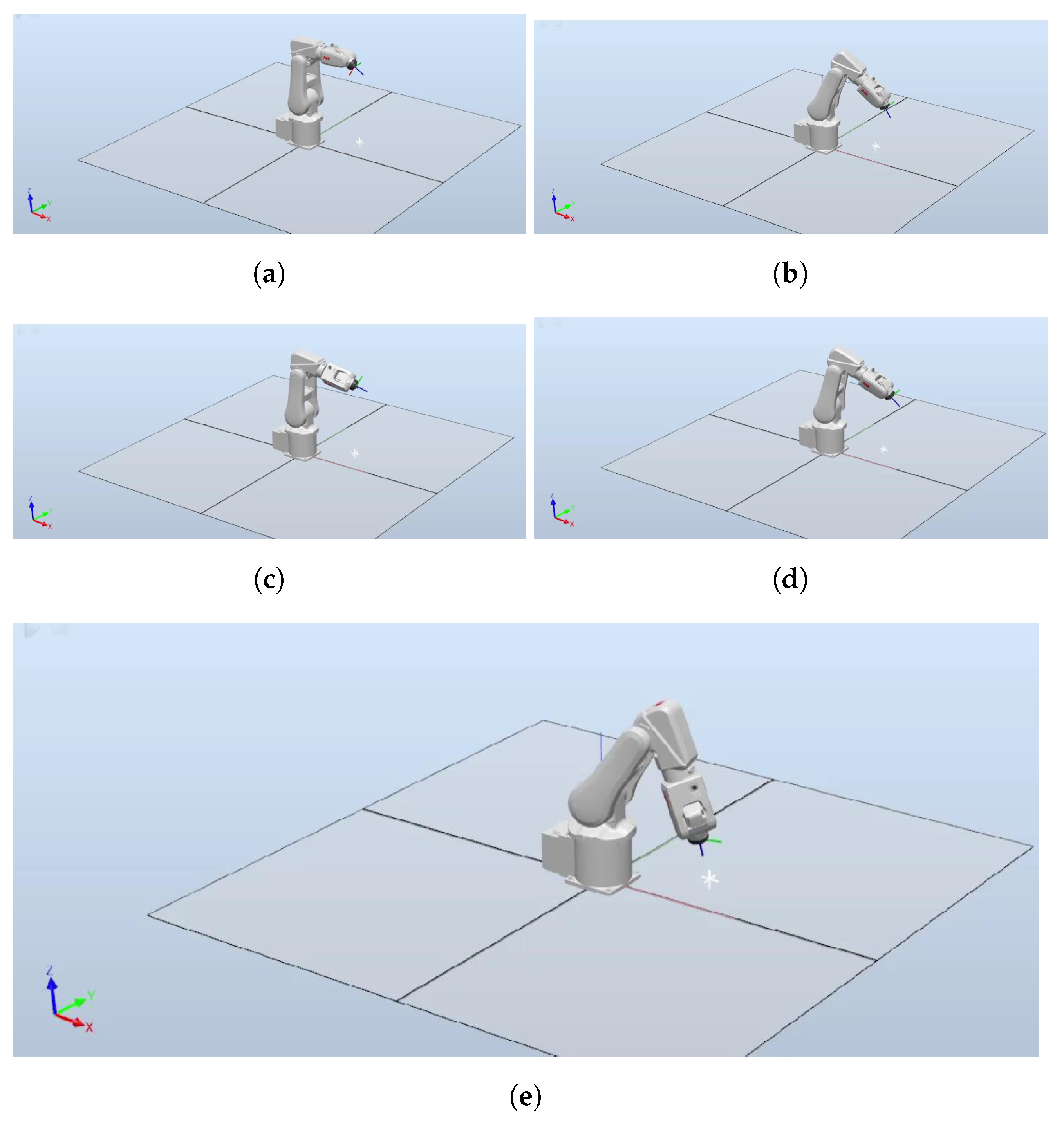
The generated trajectories were applied within the RobotStudio software in order to illustrate a possible path obtained from the method. Twenty-five trajectory points were inserted into the simulation within the software and the simulation was run. Figure 15 shows the initial, sixth, twelfth, eighteenth, and final (twenty-fourth) trajectory points.

4. Conclusions

In this paper, the GA approach to determining Ho–Cook algorithm parameters was investigated. The results of this investigation point towards the fact that this approach is a valid alternative to analytically determining the Ho–Cook coefficients. This approach can be used in further research, with additional optimization parameters, such as energy efficiency or torque optimization for continuous path planning. Still, it is shown that GA is not capable of generating the final trajectories by itself due to the boundary conditions that need to be set in order to avoid stationary results, and Bezier spline interpolation needs to be utilized to address this. The investigation of the parameters of the algorithm shows that the algorithm has the best performance when the boundary condition is set to 0.05 and the population size is set to 10,000. The number of generations does not seem to influence the convergence point, which is shown to be between 15 and 20 generations, no matter the population size. While the results are satisfactory within the context of the research, they do not particularly improve the current state-of-the-art results in the research [13,14,15,16,17,18,19,20,21,22,23,24,25,26,27]. Still, as there is a clear lack of the Ho–Cook algorithm being used for planning, the value of the achieved results lies in the fact that it can achieve results similar to the existing ones, indicating that there is room for improvement when more advanced evolutionary or swarm-based optimization algorithms are used. The execution times of the algorithm point out that it cannot be used in online real-time planning as currently presented, with the algorithm only being usable in offline planning, where the trajectories are tuned before their application in manufacturing. Still, in the current form, the algorithm as tested is executed in a single-threaded mode, and executing the algorithm on multiple threads simultaneously could significantly improve the results. Other limitations concerning the shown approach include the need to be familiar with the Ho–Cook path planning algorithm in order to apply the GA developed in this paper, as well as the generated path not being necessarily optimal, as only a near-optimal path is guaranteed by the GA. Path planning in the demonstrated manner has certain natural limitations when compared to other methods such as the dynamic position adjustment of robotic manipulator during the operation. The paths planned in this manner are inflexible to later adjustment, as the algorithm needs to be re-run to obtain the adjusted path. This can cause issues in which only the key changes are made to the paths (e.g., new paths are calculated), as opposed to the continuous tuning of the paths for a higher efficiency (production and energy-wise) [50]. Sometimes, detailed path planning is unnecessary and simply time-consuming compared to the use of simple trajectories generated by online path planning [51]. This manner of online movement training is less skill-intensive compared to detailed offline path-planning, causing an increase in the cost [52]. Finally, fine-tuned offline planned paths such as these are only applicable in predictable environments, with a lack of capability in dynamic planning [53], which would take into account the stochastic nature of the realistic environments. The rigid planning such as that presented can cause a false sense of security, as a static environment is intrinsically assumed, which is rarely the case in real production environments, where issues that may cause faults are rife [54].
Future work in the area should focus on the testing of other evolutionary algorithms on the framework developed for GA, such as differential evolution or particle swarm optimization, to determine whether those algorithms can achieve better results.

Author Contributions

Data curation, S.B.Š., N.A.; formal analysis, N.A., I.L., Z.C.; funding acquisition, Z.C.; investigation, T.G., S.B.Š., M.G.; methodology, S.B.Š., D.Š., J.Š.; project administration, Z.C.; resources, D.Š., J.Š.; software, T.G., S.B.Š.; supervision, I.L., Z.C.; validation, D.Š., J.Š., B.F.; visualization, T.G., M.G.; writing—original draft, T.G., S.B.Š., I.L., M.G.; writing—review and editing, N.A., D.Š., J.Š., B.F., Z.C. All authors have read and agreed to the published version of the manuscript.

Funding

This research received no external funding.

Institutional Review Board Statement

Not applicable.

Informed Consent Statement

Not applicable.

Data Availability Statement

Not applicable.

Acknowledgments

This research has been (partly) supported by the CEEPUS network CIII-HR-0108, European Regional Development Fund under the grant KK.01.1.1.01.0009 (DATACROSS), project CEKOM under the grant KK.01.2.2.03.0004, Erasmus+ project WICT under the grant 2021-1-HR01-KA220-HED-000031177, and University of Rijeka scientific grants uniri-mladi-technic-22-61, uniri-mladi-technic-22-57, uniri-tehnic-18-275-1447.

Conflicts of Interest

The authors declare no conflict of interest.

References

  1. Chen, H.; Fuhlbrigge, T.; Li, X. Automated industrial robot path planning for spray painting process: A review. In Proceedings of the 2008 IEEE International Conference on Automation Science and Engineering, Washington, DC, USA, 23–26 August 2008; pp. 522–527. [Google Scholar]
  2. Raja, P.; Pugazhenthi, S. Optimal path planning of mobile robots: A review. Int. J. Phys. Sci. 2012, 7, 1314–1320. [Google Scholar] [CrossRef]
  3. Angeles, J.; Rojas, A.; Lopez-Cajun, C.S. Trajectory planning in robotic continuous-path applications. IEEE J. Robot. Autom. 1988, 4, 380–385. [Google Scholar] [CrossRef]
  4. Chettibi, T. Smooth point-to-point trajectory planning for robot manipulators by using radial basis functions. Robotica 2019, 37, 539–559. [Google Scholar] [CrossRef]
  5. Cowley, A.; Cohen, B.; Marshall, W.; Taylor, C.J.; Likhachev, M. Perception and motion planning for pick-and-place of dynamic objects. In Proceedings of the 2013 IEEE/RSJ International Conference on Intelligent Robots and Systems, Tokyo, Japan, 3–7 November 2013; pp. 816–823. [Google Scholar]
  6. Khan, A.T.; Cao, X.; Li, Z.; Li, S. Evolutionary Computation Based Real-time Robot Arm Path-planning Using Beetle Antennae Search. EAI Endorsed Trans. AI Robot. 2022, 1, 1–10. [Google Scholar] [CrossRef]
  7. Draganjac, I.; Sesar, V.; Bogdan, S.; Kovacic, Z. An internet-based system for remote planning and execution of SCARA robot trajectories. In Proceedings of the 2008 34th Annual Conference of IEEE Industrial Electronics, Orlando, FL, USA, 10–13 November 2008; pp. 3485–3490. [Google Scholar]
  8. Lengagne, S.; Mathieu, P.; Kheddar, A.; Yoshida, E. Generation of dynamic motions under continuous constraints: Efficient computation using b-splines and taylor polynomials. In Proceedings of the 2010 IEEE/RSJ International Conference on Intelligent Robots and Systems, Taipei, Taiwan, 18–22 October 2010; pp. 698–703. [Google Scholar]
  9. Lian, J.; Yu, W.; Xiao, K.; Liu, W. Cubic spline interpolation-based robot path planning using a chaotic adaptive particle swarm optimization algorithm. Math. Probl. Eng. 2020, 2020, 1849240. [Google Scholar] [CrossRef]
  10. Carrasco, J.; García, S.; Rueda, M.; Das, S.; Herrera, F. Recent trends in the use of statistical tests for comparing swarm and evolutionary computing algorithms: Practical guidelines and a critical review. Swarm Evol. Comput. 2020, 54, 100665. [Google Scholar] [CrossRef] [Green Version]
  11. Bansal, J.C.; Singh, P.K.; Pal, N.R. Evolutionary and Swarm Intelligence Algorithms; Springer: Berlin/Heidelberg, Germany, 2019; Volume 779. [Google Scholar]
  12. Baressi Šegota, S.; Anđelić, N.; Lorencin, I.; Saga, M.; Car, Z. Path planning optimization of six-degree-of-freedom robotic manipulators using evolutionary algorithms. Int. J. Adv. Robot. Syst. 2020, 17, 1729881420908076. [Google Scholar] [CrossRef] [Green Version]
  13. Shukla, P.; Kumar, H.; Nandi, G.C. Robotic grasp manipulation using evolutionary computing and deep reinforcement learning. Intell. Serv. Robot. 2021, 14, 61–77. [Google Scholar] [CrossRef]
  14. Ferigo, A.; Iacca, G.; Medvet, E. Beyond body shape and brain: Evolving the sensory apparatus of voxel-based soft robots. In Proceedings of the International Conference on the Applications of Evolutionary Computation (Part of EvoStar), Virtual Event, Germany, 20–22 April 2021; Springer: Berlin/Heidelberg, Germany; pp. 210–226. [Google Scholar]
  15. Kim, J.; Ba, D.X.; Yeom, H.; Bae, J. Gait optimization of a quadruped robot using evolutionary computation. J. Bionic Eng. 2021, 18, 306–318. [Google Scholar] [CrossRef]
  16. Liu, X.; Jiang, D.; Tao, B.; Jiang, G.; Sun, Y.; Kong, J.; Tong, X.; Zhao, G.; Chen, B. Genetic algorithm-based trajectory optimization for digital twin robots. Front. Bioeng. Biotechnol. 2022, 9, 1433. [Google Scholar] [CrossRef]
  17. Li, J.Y.; Zhan, Z.H.; Tan, K.C.; Zhang, J. A meta-knowledge transfer-based differential evolution for multitask optimization. IEEE Trans. Evol. Comput. 2021, 26, 719–734. [Google Scholar] [CrossRef]
  18. Martin, J.G.; Frejo, J.R.D.; García, R.A.; Camacho, E.F. Multi-robot task allocation problem with multiple nonlinear criteria using branch and bound and genetic algorithms. Intell. Serv. Robot. 2021, 14, 707–727. [Google Scholar] [CrossRef]
  19. Hao, K.; Zhao, J.; Wang, B.; Liu, Y.; Wang, C. The application of an adaptive genetic algorithm based on collision detection in path planning of mobile robots. Comput. Intell. Neurosci. 2021, 2021, 5536574. [Google Scholar] [CrossRef]
  20. Rahmaniar, W.; Rakhmania, A.E. Mobile Robot Path Planning in a Trajectory with Multiple Obstacles Using Genetic Algorithms. J. Robot. Control (JRC) 2022, 3, 1–7. [Google Scholar] [CrossRef]
  21. Song, B.; Wang, Z.; Zou, L. An improved PSO algorithm for smooth path planning of mobile robots using continuous high-degree Bezier curve. Appl. Soft Comput. 2021, 100, 106960. [Google Scholar] [CrossRef]
  22. Li, H.; Zhao, T.; Dian, S. Forward search optimization and subgoal-based hybrid path planning to shorten and smooth global path for mobile robots. Knowl.-Based Syst. 2022, 258, 110034. [Google Scholar] [CrossRef]
  23. García, E.; Villar, J.R.; Tan, Q.; Sedano, J.; Chira, C. An efficient multi-robot path planning solution using A* and coevolutionary algorithms. Integr. Comput.-Aided Eng. 2023, 30, 41–52. [Google Scholar] [CrossRef]
  24. Yu, Z.; Duan, P.; Meng, L.; Han, Y.; Ye, F. Multi-objective path planning for mobile robot with an improved artificial bee colony algorithm. Math. Biosci. Eng. 2023, 20, 2501–2529. [Google Scholar] [CrossRef]
  25. Wu, L.; Huang, X.; Cui, J.; Liu, C.; Xiao, W. Modified adaptive ant colony optimization algorithm and its application for solving path planning of mobile robot. Expert Syst. Appl. 2023, 215, 119410. [Google Scholar] [CrossRef]
  26. Lou, J.; Yu, X.; Chen, Y.; Sun, Z.; Zheng, P. Robot Welding Path Planning and Application Based on Graphical Computing. In Proceedings of the Seventh International Congress on Information and Communication Technology; Springer: Berlin/Heidelberg, Germany, 2023; pp. 597–605. [Google Scholar]
  27. Li, J.; Zou, L.; Luo, G.; Wang, W.; Lv, C. Enhancement and evaluation in path accuracy of industrial robot for complex surface grinding. Robot. Comput.-Integr. Manuf. 2023, 81, 102521. [Google Scholar] [CrossRef]
  28. Deng, W.; Zhang, X.; Zhou, Y.; Liu, Y.; Zhou, X.; Chen, H.; Zhao, H. An enhanced fast non-dominated solution sorting genetic algorithm for multi-objective problems. Inf. Sci. 2022, 585, 441–453. [Google Scholar] [CrossRef]
  29. Zhou, J.; Huang, S.; Zhou, T.; Armaghani, D.J.; Qiu, Y. Employing a genetic algorithm and grey wolf optimizer for optimizing RF models to evaluate soil liquefaction potential. Artif. Intell. Rev. 2022, 55, 5673–5705. [Google Scholar] [CrossRef]
  30. Budi, H.S.; Elveny, M.; Zhuravlev, P.; Jalil, A.T.; Al-Janabi, S.; Alkaim, A.F.; Saleh, M.M.; Shichiyakh, R.A. Development of an adaptive genetic algorithm to optimize the problem of unequal facility location. Found. Comput. Decis. Sci. 2022, 47, 111–125. [Google Scholar] [CrossRef]
  31. Orsag, M.; Poropat, M.; Bogdan, S. Hybrid fly-by-wire quadrotor controller. Automatika 2010, 51, 19–32. [Google Scholar] [CrossRef] [Green Version]
  32. Konjević, B.; Kovačić, Z. CONTINUOUS JERK TRAJECTORY PLANNING ALGORITHMS. In Proceedings of the International Conference on Informatics in Control, Automation and Robotics, SCITEPRESS, Noordwijkerhout, The Netherlands, 28–31 July 2011; Volume 2, pp. 481–489. [Google Scholar]
  33. Konjević, B.; Punčec, M.; Kovačić, Z. Two approaches to bounded jerk trajectory planning. In Proceedings of the 2012 12th IEEE International Workshop on Advanced Motion Control (AMC), Sarajevo, Bosnia and Herzegovina, 25–27 March 2012; pp. 1–7. [Google Scholar]
  34. Močnik, G.; Kačič, Z.; Šafarič, R.; Mlakar, I. Capturing Conversational Gestures for Embodied Conversational Agents Using an Optimized Kaneda–Lucas–Tomasi Tracker and Denavit–Hartenberg-Based Kinematic Model. Sensors 2022, 22, 8318. [Google Scholar] [CrossRef]
  35. Shim, S.; Lee, S.; Joo, S.; Seo, J. Denavit-Hartenberg Notation-Based Kinematic Constraint Equations for Forward Kinematics of the 3–6 Stewart Platform. J. Mech. Robot. 2022, 14, 054505. [Google Scholar] [CrossRef]
  36. Baressi Šegota, S.; Anđelić, N.; Šercer, M.; Meštrić, H. Dynamics Modeling of Industrial Robotic Manipulators: A Machine Learning Approach Based on Synthetic Data. Mathematics 2022, 10, 1174. [Google Scholar] [CrossRef]
  37. Milenkovic, P.; Wang, Z.; Rodriguez, J.I. Encountering singularities of a serial robot along continuous paths at high precision. Mech. Mach. Theory 2023, 181, 105224. [Google Scholar] [CrossRef]
  38. Katoch, S.; Chauhan, S.S.; Kumar, V. A review on genetic algorithm: Past, present, and future. Multimed. Tools Appl. 2021, 80, 8091–8126. [Google Scholar] [CrossRef]
  39. Han, S.; Xiao, L. An improved adaptive genetic algorithm. SHS Web Conf. 2022, 140, 01044. [Google Scholar] [CrossRef]
  40. Wang, B.; Yao, X.; Jiang, Y.; Sun, C.; Shabaz, M. Design of a real-time monitoring system for smoke and dust in thermal power plants based on improved genetic algorithm. J. Healthc. Eng. 2021, 2021, 7212567. [Google Scholar] [CrossRef]
  41. Ibrahim, M.; Nurhakiki, F.; Utama, D.; Rizaki, A. Optimised genetic algorithm crossover and mutation stage for vehicle routing problem pick-up and delivery with time windows. In Proceedings of the IOP Conference Series: Materials Science and Engineering, Sanya, China, 12–14 November 2021; Volume 1071, p. 012025. [Google Scholar]
  42. Damia, A.; Esnaashari, M.; Parvizimosaed, M. Adaptive Genetic Algorithm Based on Mutation and Crossover and Selection Probabilities. In Proceedings of the 2021 7th International Conference on Web Research (ICWR), Tehran, Iran, 19–20 May 2021; pp. 86–90. [Google Scholar]
  43. Saadaoui, D.; Elyaqouti, M.; Assalaou, K.; Lidaighbi, S. Parameters optimization of solar PV cell/module using genetic algorithm based on non-uniform mutation. Energy Convers. Manag. X 2021, 12, 100129. [Google Scholar] [CrossRef]
  44. Sohail, A. Genetic algorithms in the fields of artificial intelligence and data sciences. Ann. Data Sci. 2021, 1–12. [Google Scholar] [CrossRef]
  45. Bhattacharjee, P.; Jana, R.K.; Bhattacharya, S. A Comparative Study of Dynamic Approaches for Allocating Crossover and Mutation Ratios for Genetic Algorithm-based Optimization of Wind Power Generation Cost in Jafrabad Region in India. In Proceedings of the International Conference on “Recent Advancements in Science, Engineering & Technology, and Management, Nagpur, India, 25–26 March 2021. [Google Scholar]
  46. Avdeenko, T.; Serdyukov, K. Genetic Algorithm Fitness Function Formulation for Test Data Generation with Maximum Statement Coverage. In Proceedings of the International Conference on Swarm Intelligence, Qingdao, China, 17–21 July 2021; Springer: Berlin/Heidelberg, Germany, 2021; pp. 379–389. [Google Scholar]
  47. Fogel, D.B. Evolutionary algorithms in theory and practice. Complexity 1997, 2, 26–27. [Google Scholar] [CrossRef]
  48. Liu, J.; Jin, B.; Yang, J.; Xu, L. Sea surface temperature prediction using a cubic B-spline interpolation and spatiotemporal attention mechanism. Remote Sens. Lett. 2021, 12, 478–487. [Google Scholar] [CrossRef]
  49. Tayebi, S.; Momani, S.; Arqub, O.A. The cubic B-spline interpolation method for numerical point solutions of conformable boundary value problems. Alex. Eng. J. 2022, 61, 1519–1528. [Google Scholar] [CrossRef]
  50. Gigras, Y.; Gupta, K. Artificial intelligence in robot path planning. Int. J. Soft Comput. Eng. (IJSCE) 2012, 2, 2231–2307. [Google Scholar]
  51. Liu, M. Robotic online path planning on point cloud. IEEE Trans. Cybern. 2015, 46, 1217–1228. [Google Scholar] [CrossRef]
  52. Xie, Z.; Zhang, Q.; Jiang, Z.; Liu, H. Robot learning from demonstration for path planning: A review. Sci. China Technol. Sci. 2020, 63, 1325–1334. [Google Scholar] [CrossRef]
  53. Bonny, T.; Kashkash, M. Highly optimized Q-learning-based bees approach for mobile robot path planning in static and dynamic environments. J. Field Robot. 2022, 39, 317–334. [Google Scholar] [CrossRef]
  54. Anđelić, N.; Car, Z.; Šercer, M. Neural Network-Based Model for Classification of Faults During Operation of a Robotic Manipulator. Teh. Vjesn. 2021, 28, 1380–1387. [Google Scholar]
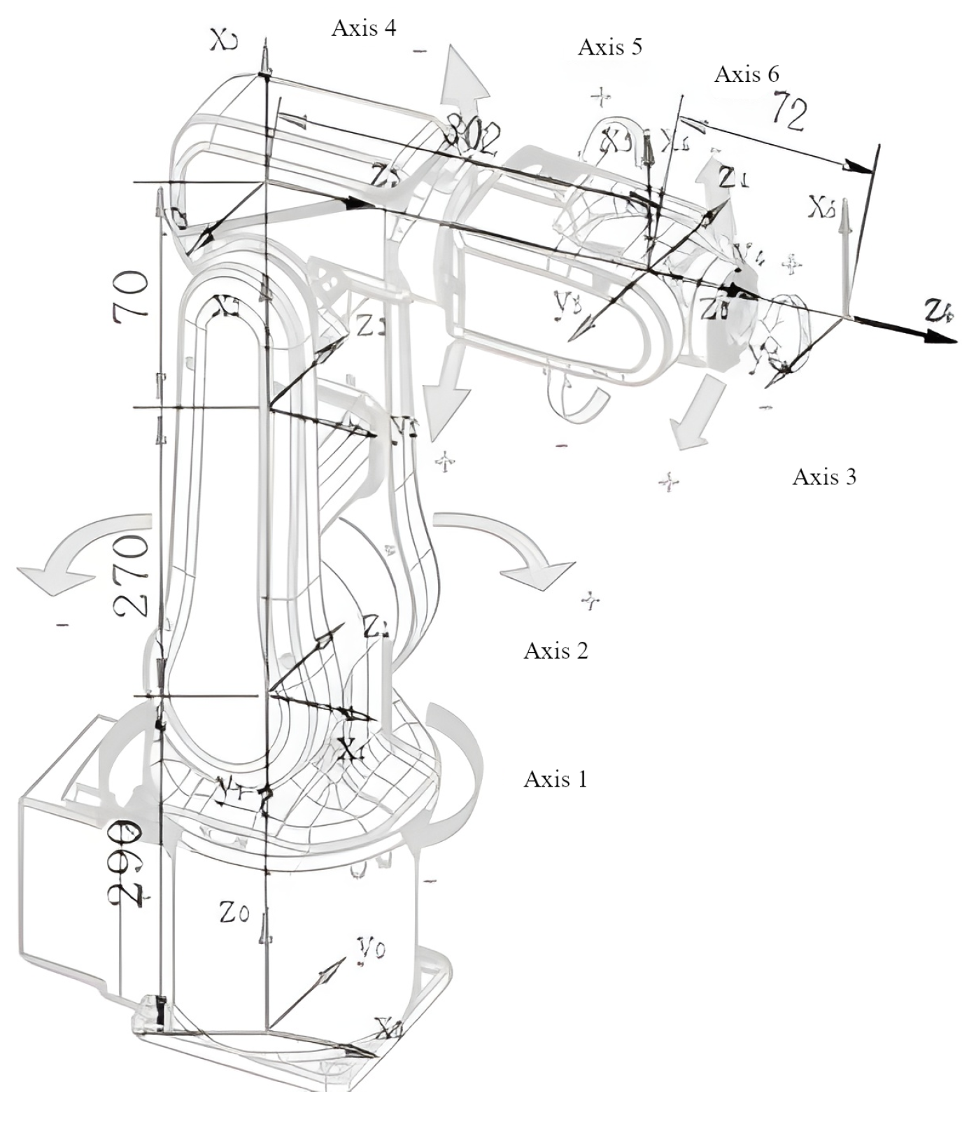
Figure 1. Simplified kinematic schematic of the ABB IRB 120 robot, with the associated D-H orthonormal coordinate systems.
Machines 11 00167 g001
Figure 2. An illustration of the recombination methodology used, where (A,B) represent two candidate solutions selected from the existing population and (C) presents the resulting candidate solution after the crossover between (A) and (B) is performed.
Machines 11 00167 g002
Figure 3. An illustration of the mutation methodology used, where (A) is the randomly selected candidate solution from the population and (B) is the randomly modified solution.
Machines 11 00167 g003
Figure 4. The illustration of the fitness function, which is the sum of the distances between the first and the last elements of the segments, as indicated with red arrows.
Machines 11 00167 g004
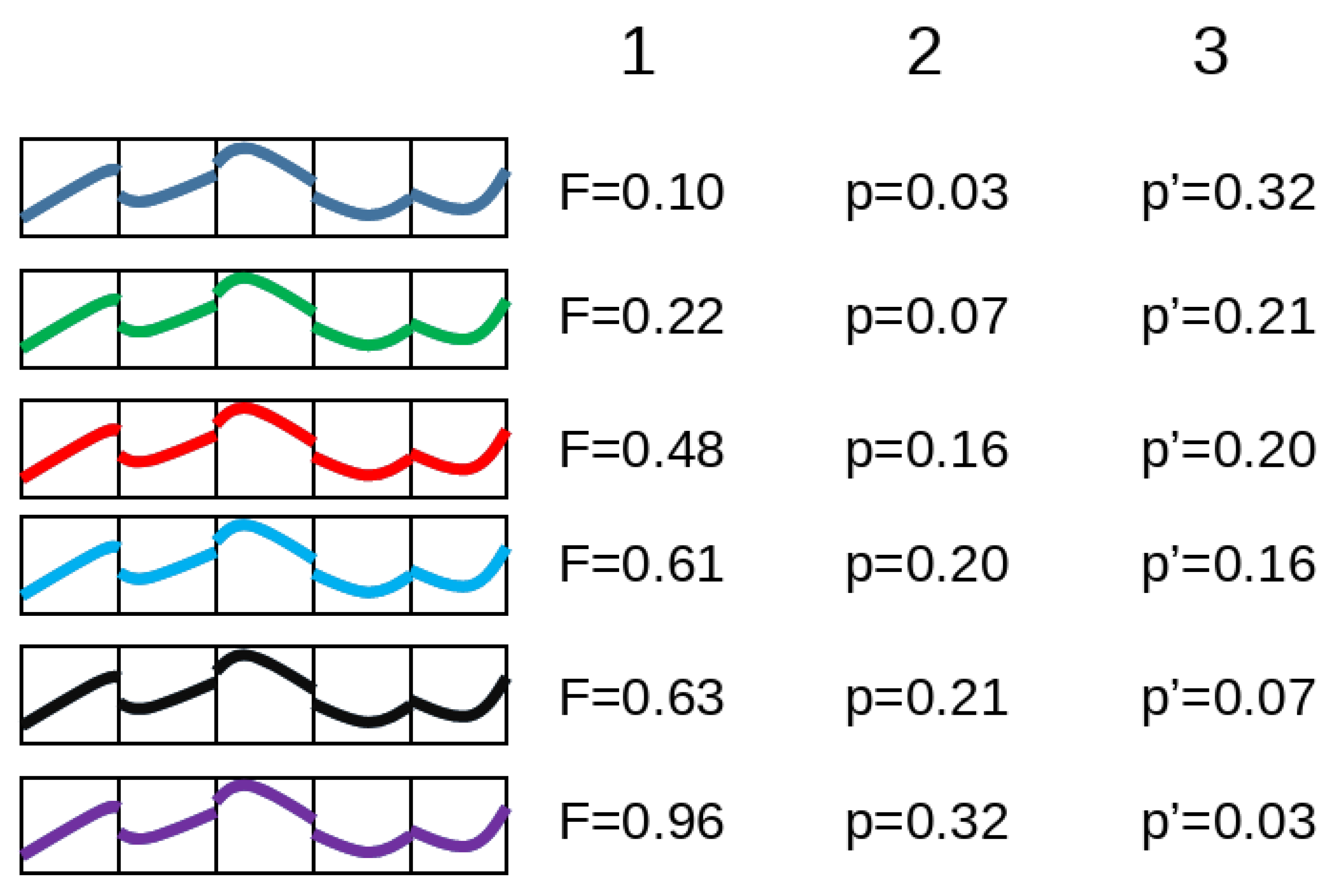
Figure 5. An illustration of the roulette wheel selection process. In step (1) the fitness is calculated according to Equation (20) (lower is better). Then, in (2), the probability is calculated as the percentage of the total population fitness (in the illustration, the total sum of individual fitness is 3.0). Finally, due to the minimization problem being observed, the probability vector is inverted in (3).
Machines 11 00167 g005
Figure 6. The behavior of the algorithm without setting the boundary condition. The best-achieved solution is visualized on the (left), and the fitness change through generations is on the (right).
Machines 11 00167 g006
Figure 7. The behavior of the algorithm for the boundary condition set to 0.2. The best-achieved solution is visualized on the (left), and the fitness change through generations is on the (right).
Machines 11 00167 g007
Figure 8. The behavior of the algorithm for the boundary condition set to 0.1. The best-achieved solution is visualized on the (left), and the fitness change through generations is on the (right).
Machines 11 00167 g008
Figure 9. The behavior of the algorithm for the boundary condition set to 0.05. The best-achieved solution is visualized on the (left), and the fitness change through generations is on the (right).
Machines 11 00167 g009
Figure 10. The behavior of the algorithm for the boundary condition set to 0.005. The best-achieved solution is visualized on the (left), and the fitness change through generations is on the (right).
Machines 11 00167 g010
Figure 11. The achieved results for the GA with 100 candidate solutions trained for 100 generations. The best-achieved solution is visualized on the (left), and the fitness change through generations is on the (right).
Machines 11 00167 g011
Figure 12. The achieved results for the GA with 1000 candidate solutions trained for 50 generations. The best-achieved solution is visualized on the (left), and the fitness change through generations is on the (right).
Machines 11 00167 g012
Figure 13. The achieved results for the GA with 10,000 candidate solutions trained for 20 generations. The best-achieved solution is visualized on the (left), and the fitness change through generations is on the (right).
Machines 11 00167 g013
Figure 14. The illustration of the interpolation process.
Machines 11 00167 g014
Figure 15. An illustration of the generated path. (a) The initial step of the simulated trajectory. (b) The sixth step of the simulated trajectory. (c) The twelfth step of the simulated trajectory. (d) The eighteenth step of the simulated trajectory. (e) The twenty-fourth step of the simulated trajectory.
Machines 11 00167 g015
Table 1. The kinematic parameters of the analyzed robotic manipulator.
Θ [rad]d [mm]a [mm] α [rad]
Θ 1 = q 1 d 1 = 290 a 1 = 0 α 1 = π / 2
Θ 2 = q 2 d 2 = 0 a 2 = 270 α 2 = 0
Θ 3 = q 3 d 3 = 0 a 3 = 70 α 3 = π / 2
Θ 4 = q 4 d 4 = 302 a 4 = 0 α 4 = π / 2
Θ 5 = q 5 d 5 = 0 a 5 = 0 α 5 = π / 2
Θ 6 = q 6 d 6 = 72 a 6 = 0 α 6 = 0
Table 2. The execution times of various configurations, averaged over ten runs, with an average time per generation and the total execution time given.
PopulationGenerationsTotal Time [s]Average Time per Generation [s]
10010023.40.234
100050119.52.39
10,00020403.420.17
Disclaimer/Publisher’s Note: The statements, opinions and data contained in all publications are solely those of the individual author(s) and contributor(s) and not of MDPI and/or the editor(s). MDPI and/or the editor(s) disclaim responsibility for any injury to people or property resulting from any ideas, methods, instructions or products referred to in the content.