Abstract
Condition monitoring and fault management approaches can help with timely maintenance planning, assure industry-wide continuous production, and enhance both performance and safety in complex industrial operations. At the moment, data-driven approaches for condition monitoring and fault detection are the most attractive being conceived, developed, and applied with less of a need for sophisticated expertise and detailed knowledge of the addressed plant. Among them, Gaussian mixture model (GMM) methods can offer some advantages. However, conventional GMM solutions need the number of Gaussian components to be defined in advance and suffer from the inability to detect new types of faults and identify new operating modes. To address these issues, this paper presents a novel data-driven method, based on automated GMM (AutoGMM) and decision trees (DTree), for the online condition monitoring of electrical industrial loads. By leveraging the benefits of the AutoGMM and the DTree, after the training phase, the proposed approach allows the clustering and time allocation of nominal operating conditions, the identification of both already-classified and new anomalous conditions, and the acknowledgment of new operating modes of the monitored industrial asset. The proposed method, implemented on a commercial cloud-computing platform, is validated on a real industrial plant with electrical loads, characterized by a daily periodic working cycle, by using active power consumption data.
1. Introduction
Proper fault management approaches on real engineering systems can support timely maintenance planning, ensure industry-wide continuous production, and improve both the performance and safety of complex industrial plants and systems [1,2,3,4,5,6,7]. In this regard, condition monitoring (CM), that is to say, the process of monitoring specific parameters of industrial machinery (vibration, temperature, power consumption, etc.) in order to identify a significant change which may be indicative of a developing fault, has gained great attention recently with the help of sensor monitoring and signal processing technologies. Thanks to CM, it has become possible to plan maintenance activities, and to take actions to guarantee operational continuity of industrial machinery and to prevent serious failures which could shorten their lifespan [1,8].
CM approaches can be divided into two basic categories: physics-based methodologies and data-driven methodologies [1,9]. In order to identify the corresponding defects, physics-based approaches exploit explicit mathematical modeling and machinery/equipment specifications [10,11]. For instance, the estimation of parameters of the mathematical model of electrical motors can be useful to detect faults and monitor the health state [12,13]. However, such approaches can be complicated when used in practice because of the complexity of real plants. In data-driven approaches, the training of the model is conducted using historic data generated by the sensors installed on the machinery. At the moment, data-driven approaches are more attractive [8,14,15,16,17], being conceived, developed, and applied with less of a need for sophisticated expertise and detailed knowledge of the addressed plant. Data-driven methodologies encompass both statistical solutions (e.g., Gaussian mixture model (GMM), K-means, and Bayesian) and machine learning (ML) techniques; see, e.g., [18,19,20,21]. Among them, GMM methods can offer some advantages. In particular, they can provide more classification information for maintenance engineers (to further investigate all possible faulty components), are more computationally efficient, and require fewer training data [1,22]. Thus, they turn out to be more suitable for online CM applications [8]. However, conventional GMM solutions are affected by the following main limitations, namely, the need of defining in advance the number of Gaussian components before training and the inability to detect new types of faults and identify new operating modes. The latter can be a serious limitation since the operational setup and the environmental conditions of industrial plants can vary over time, and this can lead to new functioning modes and unforeseen anomalies [1]. Moreover, it is important to correctly classify both the normal and faulty behavior of industrial machinery by considering their temporal occurrence [23,24], since industrial plants can be subject to periodical working cycles [3].
To address the above issues from conventional GMMs, this paper presents a novel method for the online CM of electrical industrial loads, which is able to identify their regular/normal operating modes, detect anomalous working conditions, and determine new operating modes by using an active power consumption data stream. The proposed solution is essentially an online data-driven algorithm combining automated Gaussian mixture model (AutoGMM) [25,26] and decision tree (DTree) [27,28].
To the best of our knowledge, this is the first study conceiving and applying a combined AutoGMM-DTree approach to the online CM of industrial loads for both anomaly and novelty detection. The AutoGMM is employed to identify the normal operating conditions of the system by performing the online clustering of the measured power consumption data stream into stochastic Gaussian distributions, which are associated with the normal operating modes of the plant. Unlike the conventional GMM method where the number of clusters is chosen in advance by the designer [29], the proposed AutoGMM automatically determines the number of Gaussian distributions, and thus the number of the operating modes of the plant. Then, a trained DTree is used to provide a time allocation for each normal operating condition detected by the AutoGMM, and thus predict the expected power consumption level of each new sample based on its arrival time. As a result, anomalies are detected when the measured power consumption does not belong to the predicted cluster. As shown later in the paper, the resulting AutoGMM-Dtree approach is also able to merge and remove clusters, as well as converting a cluster initially believed to be anomalous into a new operating mode of the plant. To validate the proposed algorithm, an industrial scenario with electrical loads characterized by a daily periodic working cycle is considered as a case study.
To sum up, the contributions of this work are:
- The conception of a novel data-driven algorithm combining AutoGMM and decision tree (DTree).
- The application of the proposed AutoGMM-Dtree algorithm to the condition monitoring of real industrial loads, characterized by a daily periodic working cycle.
- The procedure to train the proposed algorithm in a real industrial context and its subsequent validation.
- By leveraging the benefits of the AutoGMM and the DTree, the proposed approach allows (i) the online clustering and time allocation of nominal operating conditions; (ii) the online identification of already-classified and new anomalous conditions; (iii) the online acknowledgment of new operating modes of the monitored industrial asset.
The rest of this paper is organized as follows. Section 2 presents the scenario addressed in this study, that is to say, the condition monitoring of industrial loads via a single centralized power meter. Section 3 describes the combined AutoGMM-DTree methodology, which is then validated on the addressed industrial plant in Section 4. Finally, Section 5 concludes the paper.
2. Objective of the Work and Its Industrial Application
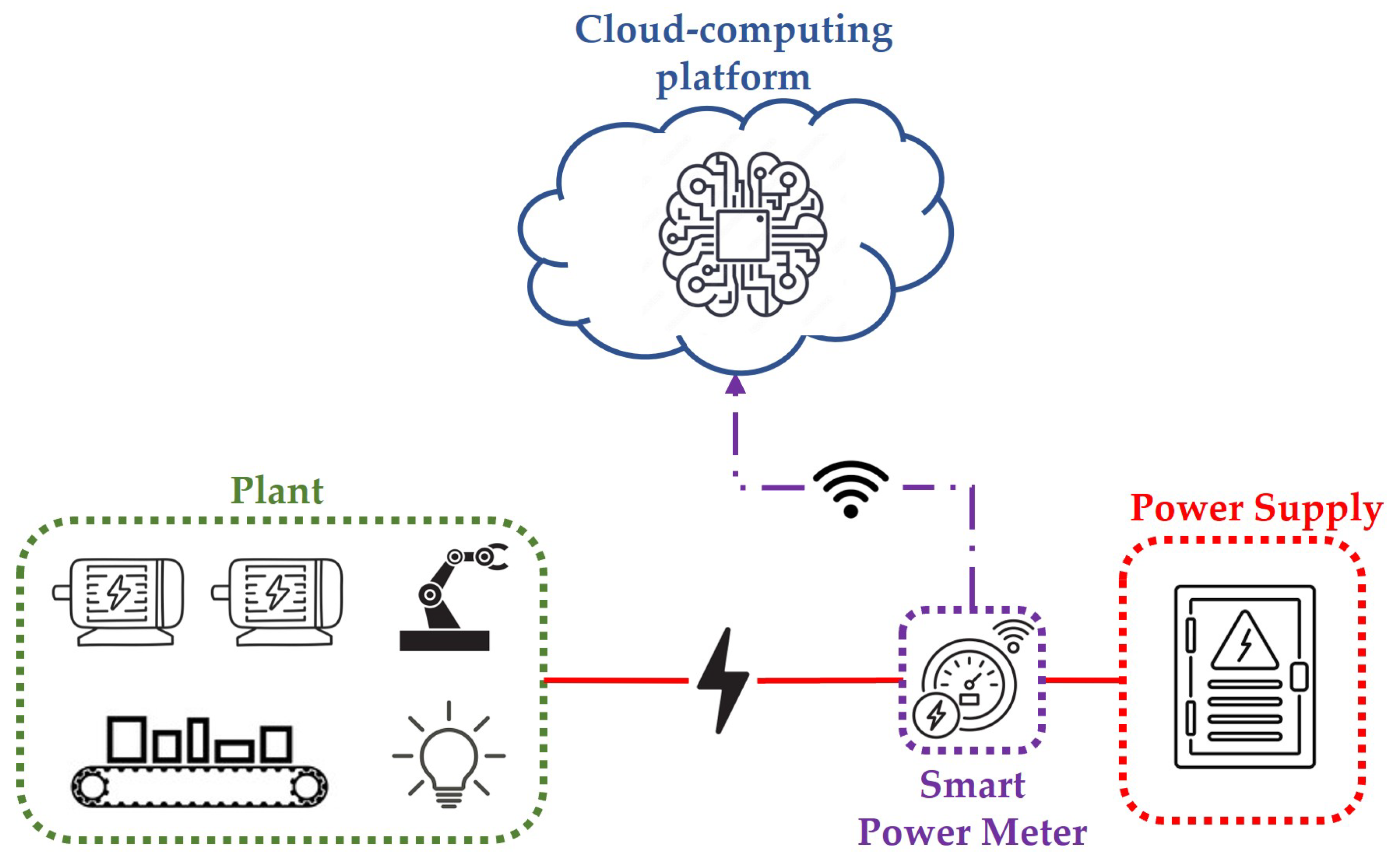
In this study, a typical scenario, shown in Figure 1, for condition monitoring of industrial loads is considered. More specifically, in such a scenario, an industrial plant consisting of electrical loads, e.g., machine tools, electrical motors, robots, or lights, characterized by a periodical power consumption, is fed by a centralized power supply. The aggregate power consumption of the electrical loads is measured by means of a single power meter, which transmits the measured time-series data to a cloud-computing platform. Finally, a software application implemented on the cloud-computing platform processes the collected time series to perform both condition monitoring and anomaly/novelty detection of the industrial plant.

Figure 1.
Schematic of the considered industrial scenario.
It is worth highlighting that in this study, compared to other solutions based on the monitoring of single loads by means of distributed power meters, the assumption of using only a single centralized power meter allows for reducing costs and increasing the simplicity of the proposed methodology. Also, note that the considered plant can be made up of either homogeneous or heterogeneous electrical loads under the hypothesis that the global power consumption is characterized by a daily periodical cycle.
Under these assumptions, the objective of this work is to design an automated algorithm able to detect the regular operating modes of the plant and to distinguish them from abnormal operating modes which may be symptomatic of failures or undesired working conditions. Additionally, considering that in common industrial scenarios the normal operating modes of the plant may be affected by variations over time, the algorithm must be able to autonomously acknowledge new operating modes, which may be added into the set of the existing ones or replace one of them.
3. The Proposed AutoGMM-DTree Methodology
To achieve the objective stated in the previous section, in this work, an online algorithm based on AutoGMM coupled with a trained DTree is designed. The AutoGMM is employed to automatically model the probability distribution of active power measurement data collected from the power meter using a combination of Gaussian distributions. Its main task is to identify the normal operating conditions of the system by performing online clustering of the data stream. Instead, the DTree is employed to provide a time allocation for the normal operating conditions detected by the AutoGMM and to predict the expected active power of each new sample based on its arrival time. In this way, anomalies are automatically detected when a mismatch between the actual and the predicted active power occurs.
3.1. AutoGMM-Based Method for Operating Mode Clustering
The GMM method is well-suited for clustering the collected data into distributions that describe the normal operating modes of the plant. Subsequently, this method assigns a probability to each data point to belong to the Gaussian clusters. All the same, an AutoGMM is used because the number of regular operating modes of the plant might not be known beforehand or might change over time. Differently from the conventional GMM method, where the number of clusters is chosen in advance by the designer, the proposed AutoGMM automatically determines online the optimal number of Gaussian distributions which matches the operating modes of the plant. Before introducing the iterative method adopted by the AutoGMM to determine the clusters, it is convenient to define the following parameters which characterize each i-th Gaussian distribution in the mixture:
- Mean (): It represents the center of the Gaussian distribution and defines the location of the peak or center of the cluster.
- Variance (): It defines the width of the Gaussian distribution.
- Weight (): It determines the weight or importance of the Gaussian distribution. It represents the probability of a data point belonging to the i-th cluster.
3.1.1. Procedure for the Cluster Update
Figure 2 represents the iterative online procedure of the AutoGMM triggered by the arrival of each new active power measurement data point. This procedure is based on clusters characterized by a time window of samples. In particular, the AutoGMM is initialized with a single cluster with , and with arbitrarily chosen. The first step evaluates the new data point as an inlier or outlier. To perform this evaluation, the z-score is computed for each i-th cluster as follows:
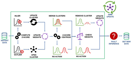
Figure 2.
The evolution of the GMM model upon the arrival of each new measurement.
The data point is identified as an inlier if there exists i such that , according to the so-called three-sigma rule of thumb. If i is unique, belongs to the i-th cluster. Otherwise, if i is not unique, belongs to the i-th cluster with the minimum . Finally, if an i does not exists such that , is identified as an outlier.
After this step, the parameters of the clusters are updated. If belongs to the i-th cluster, the mean, and variance of this cluster are updated as follows [25]:
where represents the learning rate, is the mean of the cluster i at the time instant , is the variance of the cluster i, and is the weight of the cluster i.
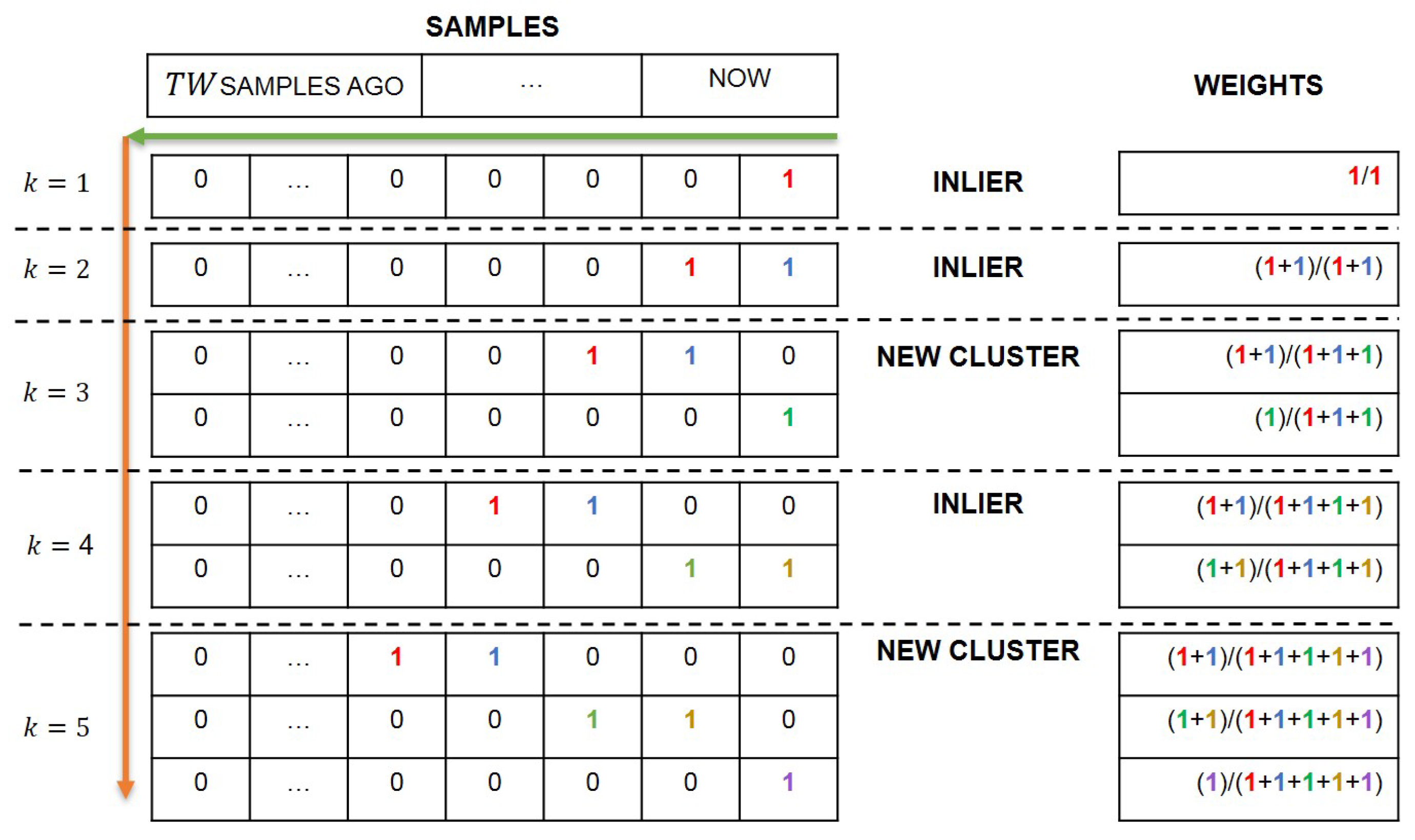
Instead, the Gaussian weights are updated according to the procedure depicted in Figure 3. To each cluster, a time window of samples is associated. Thus, referring to Figure 3, a matrix H of size is constructed, where denotes the current number of clusters. The last column of H is referred to as the current sample in time instant . When a new sample is acquired, if it belongs to the i-th cluster according to the z-score (1), 1 is placed in the last column of the i-th row, while in the last column of all the other rows is placed a 0. However, if the sample does not belong to any cluster, a new row is added to the matrix H, defining a new cluster. In both cases, the other columns of H are shifted by one position to the left, and the first columns are canceled. Note that, initially, the matrix H is defined by a single row () with zero elements and each new row has zero elements except for the last column. After this procedure, the weight of each cluster i at the sample k, is calculated with the following formula:
with
where represents the element of the i-th row and j-th column of the matrix H. It is worth remarking that in the defined AutoGMM algorithm, each cluster represents an operating mode. When a measurement does not belong to any of the existing clusters, the newly initialized cluster will have an initial weight dependent on the number of acquired samples, which at steady-state, since observations have been collected, is equal to . From that moment on, each observation that falls into that cluster contributes to increasing its weight at the expense of the other clusters, because the sum of the weights of all clusters must be equal to 1.
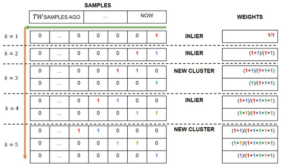
Figure 3.
Evolution of the AutoGMM clusters.
3.1.2. Procedure for Cluster Removal and Mergers
After updating the weights, a procedure to merge or remove clusters is performed. The first step of this procedure evaluates the possibility of merging clusters with similar means. This evaluation is based on calculating the following z-score for each , :
Clusters with i and j such that or , are merged, where is a tuning positive parameter, equal to 3 (three-sigma rule of thumb). If this condition is verified, the data flow is leading the cluster towards the same distribution as another cluster. Therefore, these two clusters are merged into a single cluster as it is assumed that they are representative of the same distribution. If two clusters i and j are merged at step k, the cluster l obtained by the merging of the two clusters assumes the following parameters:
Subsequently, a weight check is performed to evaluate the need for removing a cluster. A parameter is defined, so any cluster with a weight lower than this value for consecutive samples is removed, with . In this study, is chosen to be equal to .
3.2. Anomaly and Novelty Detection Based on DTree
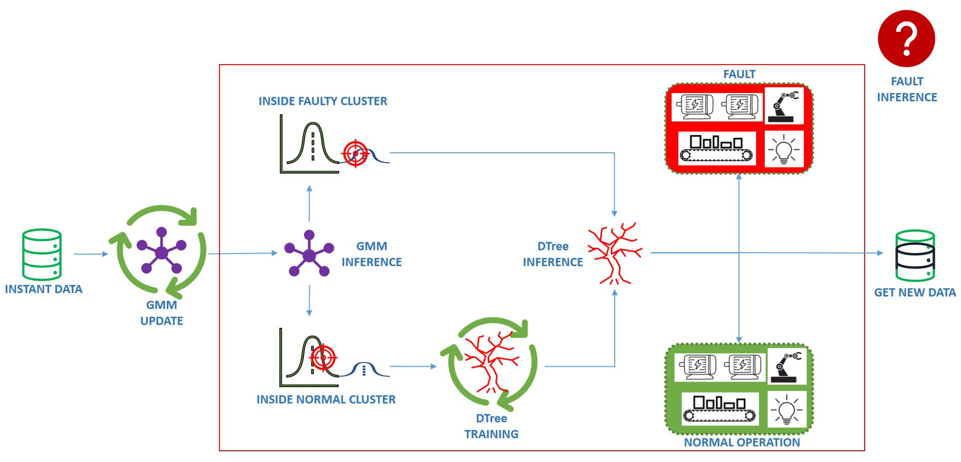
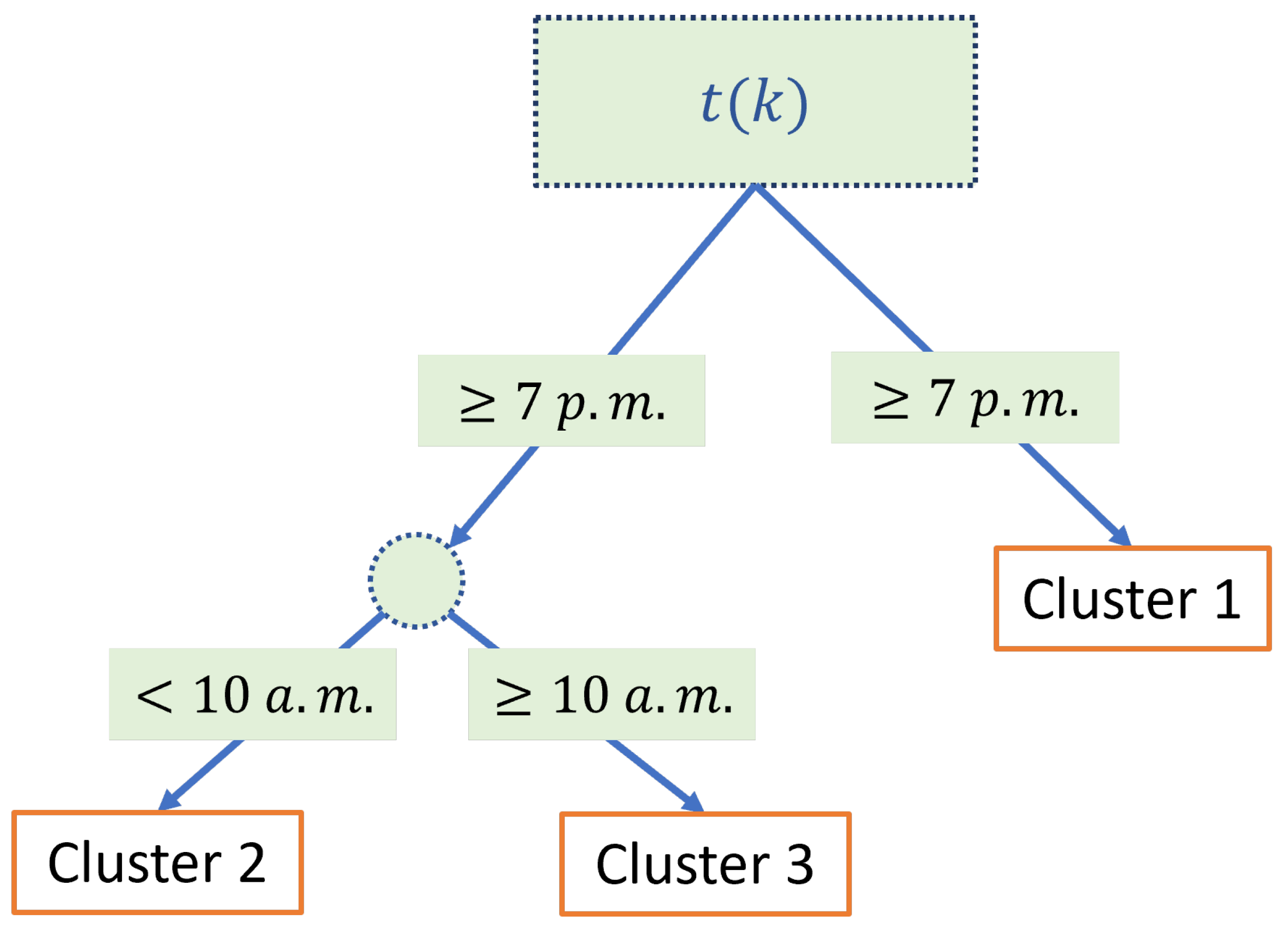
Once the parameters of AutoGMM have been updated, anomaly and novelty detection are performed, as reported in Figure 4. A DTree is trained to predict the normal cluster of membership, i.e., the cluster to which the sample k should belong based on its arrival time . The DTree is a classifier expressed as a recursive partition of the instance space. It is based on a hierarchical tree structure, which consists of a root node, branches, and inner and leaf nodes [30]. The latter represent the possible outcomes within the space. In this work, the adopted training criteria for the DTree is the Gini index and the chosen value of the complexity parameter which regulates the overfitting is 0.1. The DTree is trained only using samples belonging to normal clusters, i.e., clusters that have a weight , where is a user-defined threshold. By training the DTree using only samples belonging to normal clusters, a correlation between the sample arrival time and the active power of normal clusters is registered. For instance, a diagram of a trained DTree with three leaf nodes (the predicted clusters) showing the time-based inference of the expected clusters is reported in Figure 5. As can be seen, the input of the DTree is the arrival time of the new sample while its output is the expected cluster of membership of the new sample. It is worth highlighting that the training algorithm of the DTree also exploits the active power measurements to adaptively change the expected clusters during the operation of the plant.

Figure 4.
DTree training and fault inference.
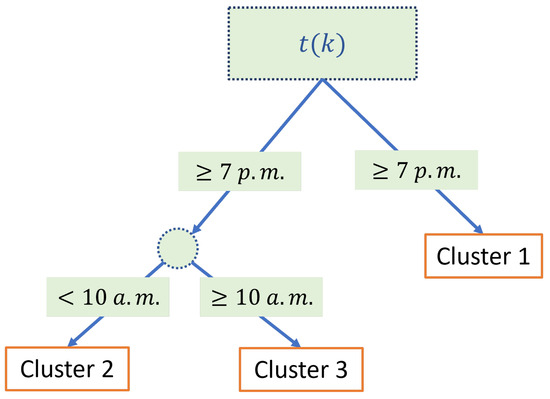
Figure 5.
Example of a trained DTree for operating mode prediction.
Note that not all the normal clusters are clusters expected by the DTree. Only the clusters expected by the DTree can be considered representative of normal operating modes of the plant. Hence, an anomaly is registered every time the current sample does not belong to the cluster predicted by the DTree. In particular, any cluster that has never reached the weight defined by the hyperparameter represents a potential fault, and it requires further investigation to determine whether it is a fault or simply a new operating mode of the plant. Such a cluster is identified as a faulty cluster, meaning a cluster suspected of being a system fault. If a faulty cluster reaches the threshold and becomes a cluster expected by the DTree, it is interpreted as a normal operating mode of the plant. So, the weight calculation (5) is very important as it is the main discriminant for fault detection and new operating mode identification.
4. Experiments and Results
4.1. Case Study and Experimental Setup
The proposed algorithm has been developed and implemented in order to be easily embedded and deployed within a specialized hardware setup (DIRAC monitor IoT system, DMIS) for the monitoring and energy efficiency of industrial plants to the extent of the industrial R&D project DIRAC (specifically its equipment modeling system module EqMS).
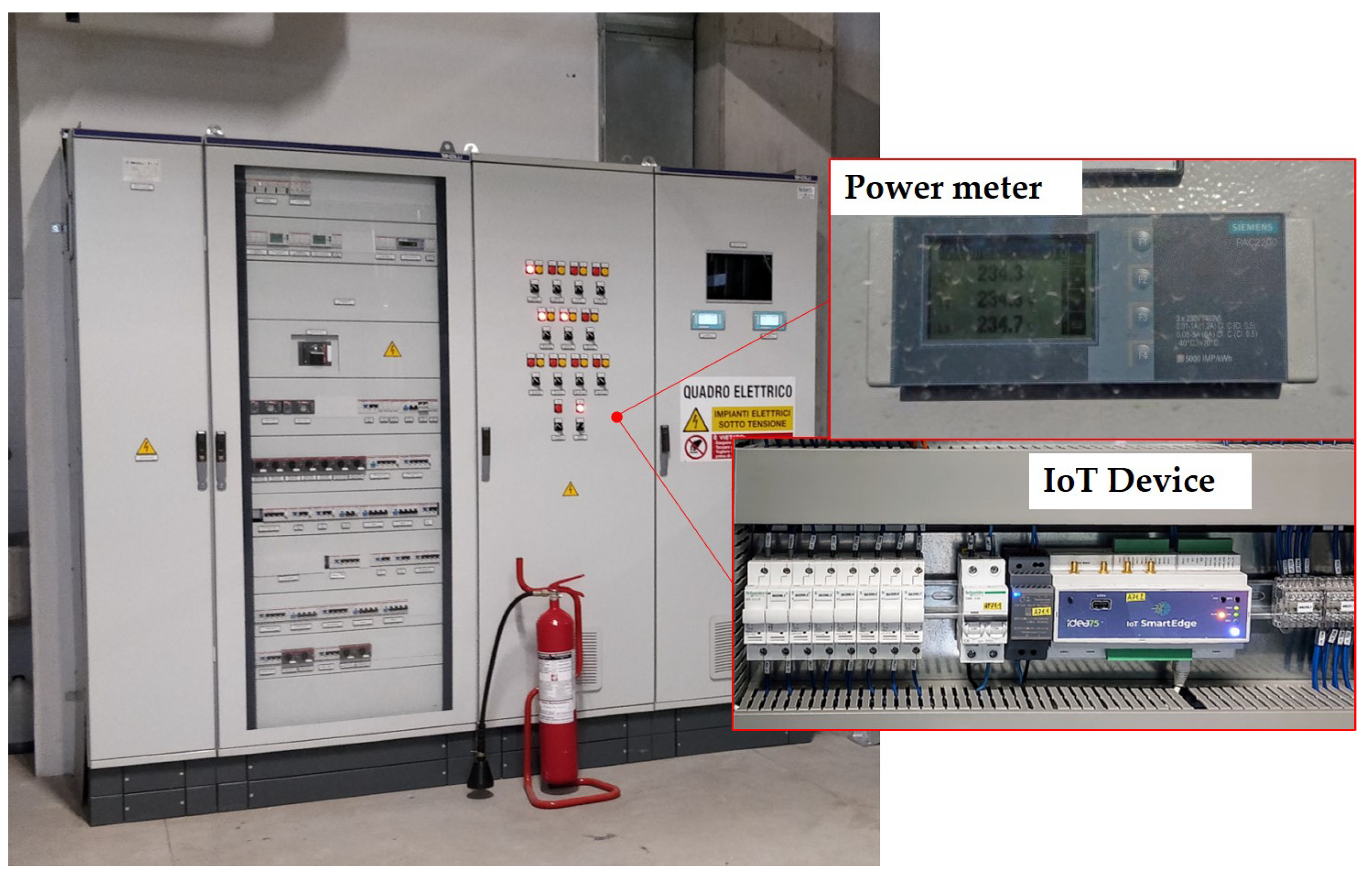
To validate the proposed algorithm, an industrial plant operated by Free Energy Saving srl and characterized by a daily periodic working cycle is considered as a case study. The same plant may be chosen in the future as a case study for the validation of the hardware prototypes and the DMIS developed within the DIRAC project. A view of the electrical cabinet which supplies the plant where the smart meter is installed is shown in Figure 6. The power meter is a Siemens SENTRON, 7KM PAC2200, whose measurements are collected by an IoT device and sent to a cloud platform, where the proposed AutoGMM-DTree algorithm is implemented by adopting AWS Amazon EC2 C5 instances, model c5d.xlarge.
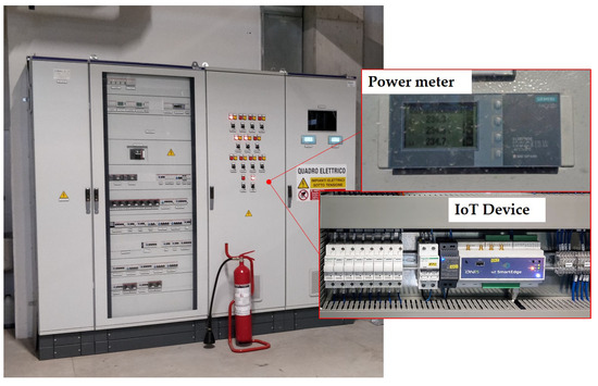
Figure 6.
Electrical cabinet which supplies the plant operated by Free Energy Saving srl.
4.2. Performance Comparison with a Conventional 2D GMM
Before the analysis of the experimental results, a comparison between the proposed algorithm and a more conventional approach based on a 2D GMM on a synthetic dataset is presented. The 2D GMM, differently from the proposed AutoGMM, is trained using two different inputs: the active power value and the hour of the day in which the sample has been collected. The training of the 2D GMM is based on formulas similar to (1)–(4) and modified for a two-dimensional case. In particular, the z-score is substituted by the Mahalanobis distance [31]:
where is the vector of the inputs of the k-th sample, is the mean vector of the i-th cluster at the -th sample and is the covariance matrix which substitutes the variance defined in the one-dimensional case. A sample is considered an inlier for a cluster when .
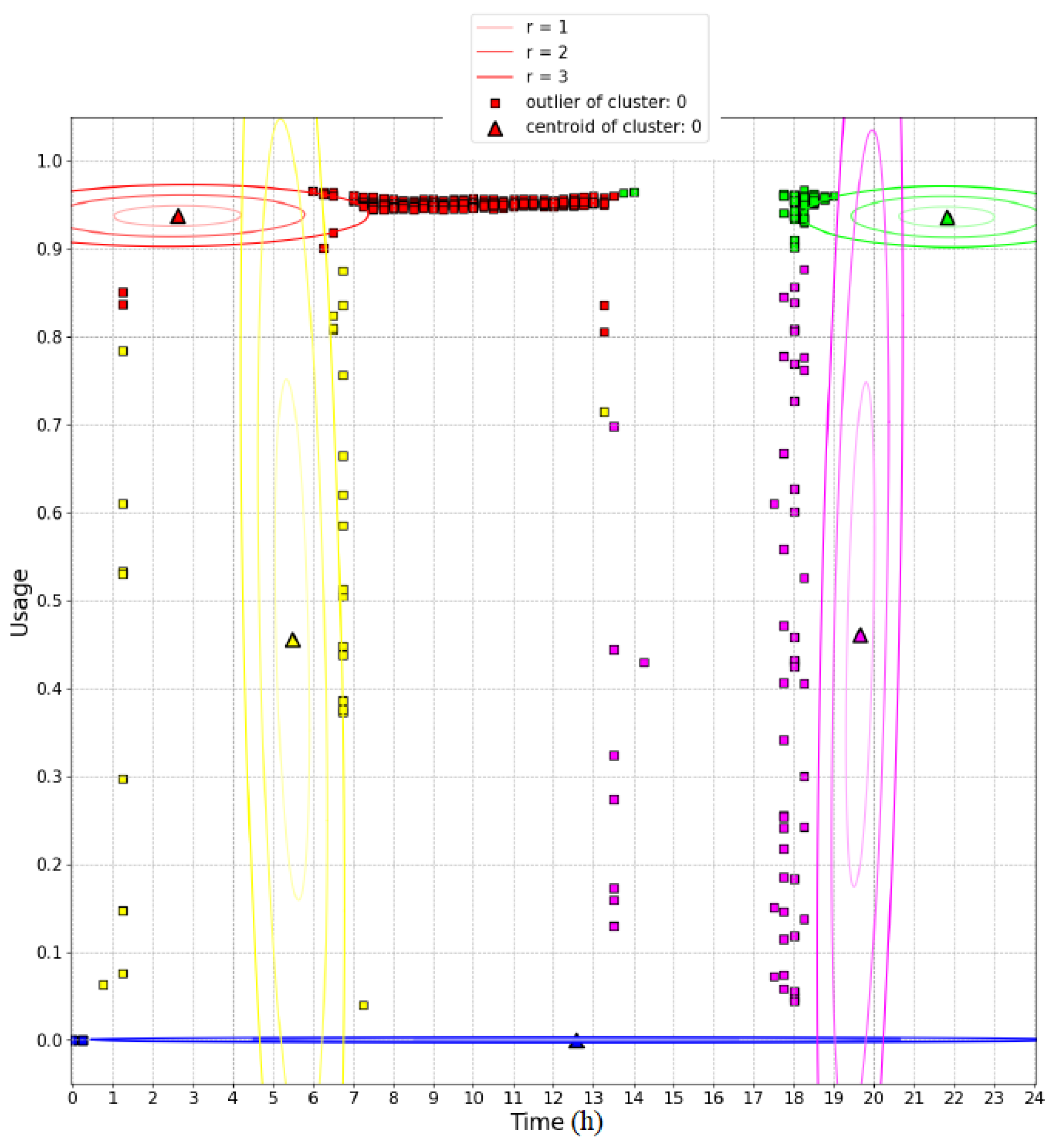
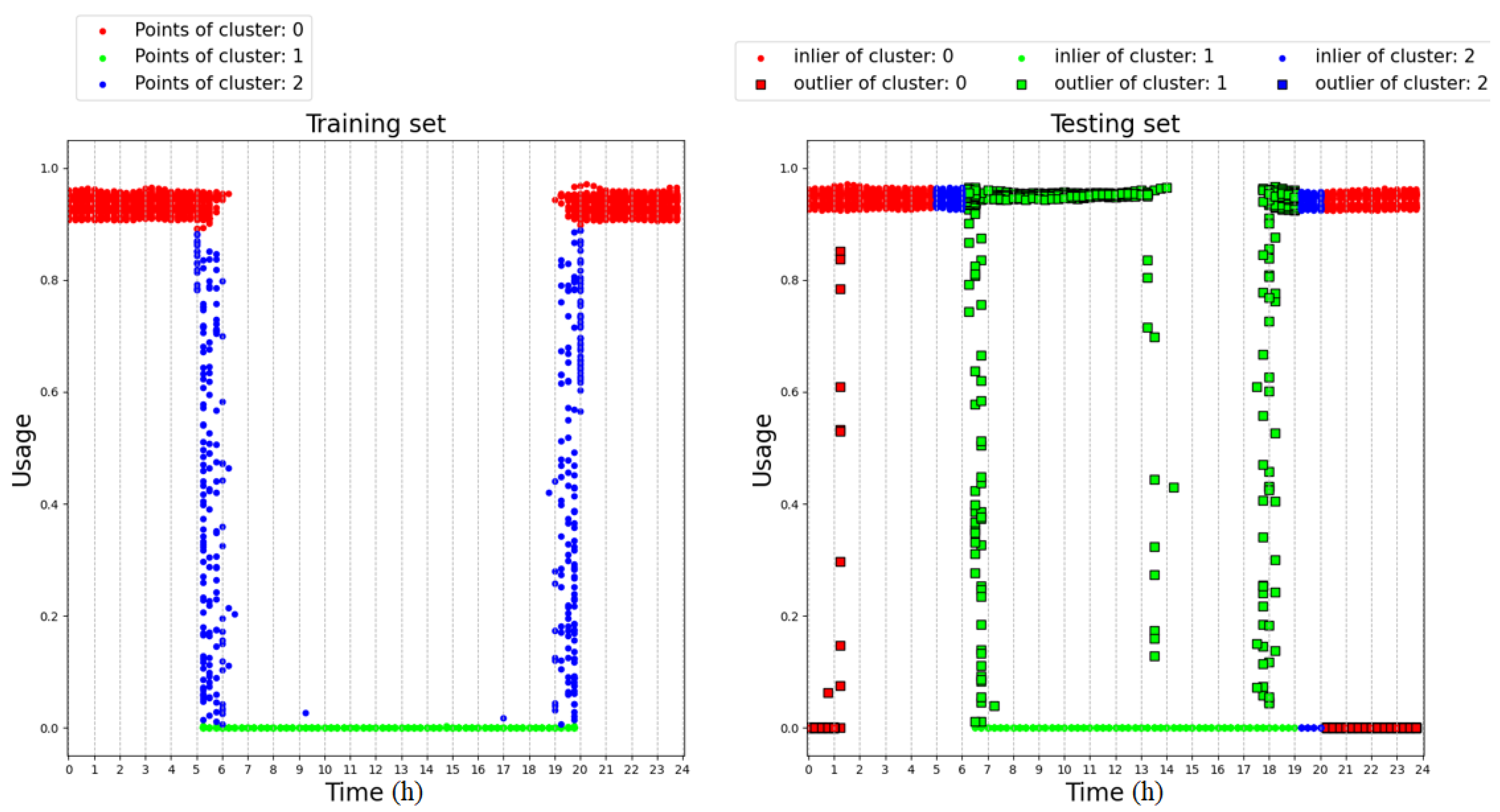
The left-hand side of Figure 7 shows the training dataset used to train the 2D GMM and the centroids of five clusters defined a priori. The right-hand side of the figure shows the results achieved on a testing set which includes anomalies with respect to the training set. In this figure, the circles represent samples recognized as inliers while the squares represent outliers. The color of the outliers is inherited from the cluster with the lowest Mahalanobis distance. As can be seen, the algorithm fails in recognizing as outliers the blue samples collected in the time range 0–1.5 h. The same error occurs with the blue samples collected in the time range 20–24 h. This can be explained by observing Figure 8, which illustrates the 2D probability density functions of the clusters trained with the training dataset. For each cluster, three ellipses denoting Mahalanobis distances from the centroid equal to 1, 2, and 3 are drawn. In particular, the blue cluster spans the whole time range. This is due to the intrinsic assumption that the GMM is dealing with normal distributions of the inputs, while in this case the distribution of the time feature is strictly rectangular, as shown in the training set. This incongruence leads all the clusters to over-range the time intervals in which the samples have been collected, as can be observed by comparing the time extension of the clusters in Figure 8 and the time ranges of the samples of the training set shown in Figure 7.
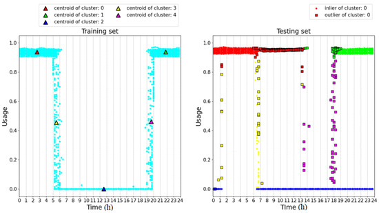
Figure 7.
Analysis of the 2D GMM on a synthetic dataset.
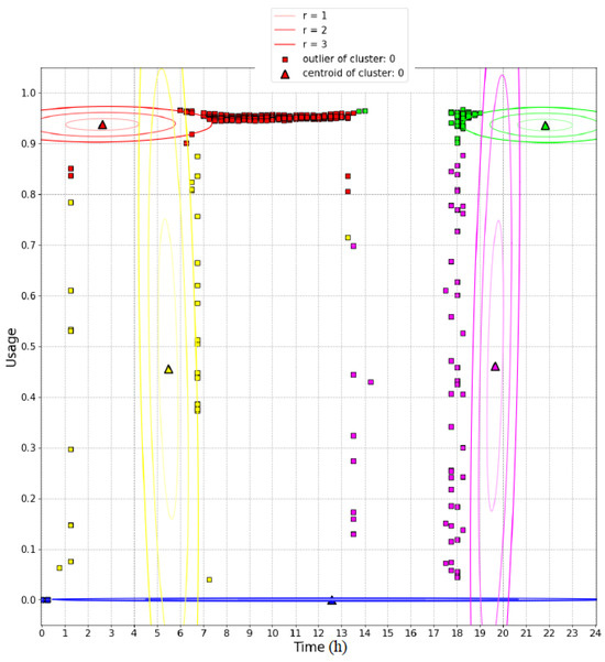
Figure 8.
2D probability density functions of the clusters of the 2D GMM.
Figure 9 shows the results obtained by means of the proposed algorithm on the same dataset and adopting a predefined number of clusters. Only three clusters are chosen since, in this case, only the active power is used as an input for the GMM. The figure on the right shows how the DTree correctly recognizes as outliers the samples collected in the time ranges 0–1.5 h and 20–24 h, thus overcoming the performance of the conventional 2D GMM. In this case, the effectiveness of the proposed algorithm is ensured by the fact that the DTree learns a relationship between the clusters of the GMM and the arrival time of the samples, overcoming the assumption of the normal distribution of the time feature, which is intrinsic in the 2D GMM.
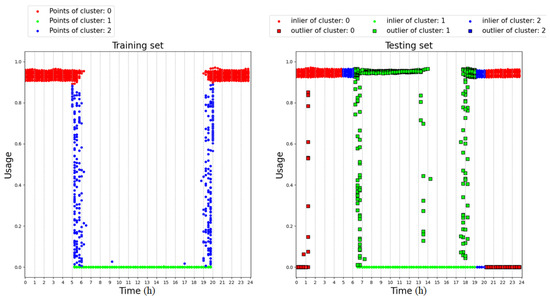
Figure 9.
Analysis of the proposed algorithm on a synthetic dataset.
4.3. Results on the Experimental Setup
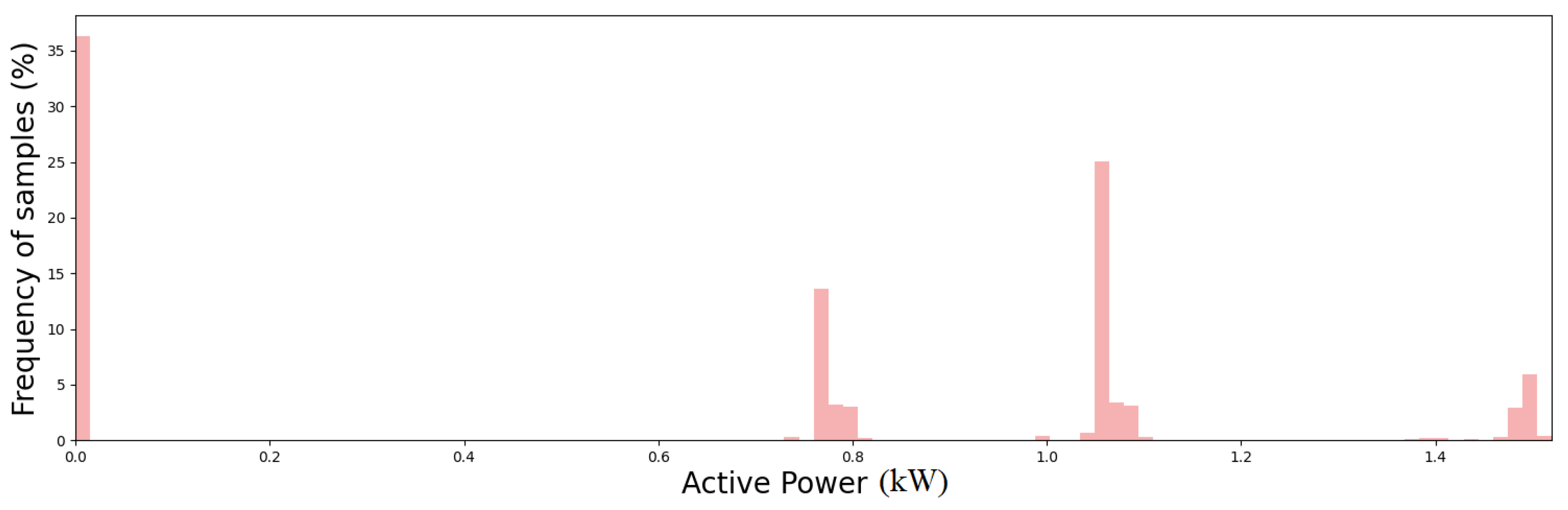
The full capability of the proposed algorithm in detecting outliers and novel operating modes is demonstrated by analyzing the results achieved on the experimental dataset. In particular, active power time series collected for a year and a half with a sampling time of 30 min have been collected and processed by the proposed algorithm. Figure 10 shows the frequency distribution of the active power consumption of the whole dataset. Note that different levels of active power over the observation period are registered. Figure 11 shows the active power time series for 50 days. Note that at day 20 an anomaly in the power consumption with respect to the previous and following days can be observed. Another anomaly can be observed at day 55. It is also important to draw attention to the sudden change in the plant’s operating modes starting on day 36. The zoomed figures shows the daily periodic working cycles of the plant.

Figure 10.
Frequency distribution of active power consumption for the whole dataset.
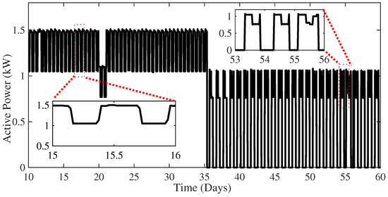
Figure 11.
Active power time-series data for 50 days.
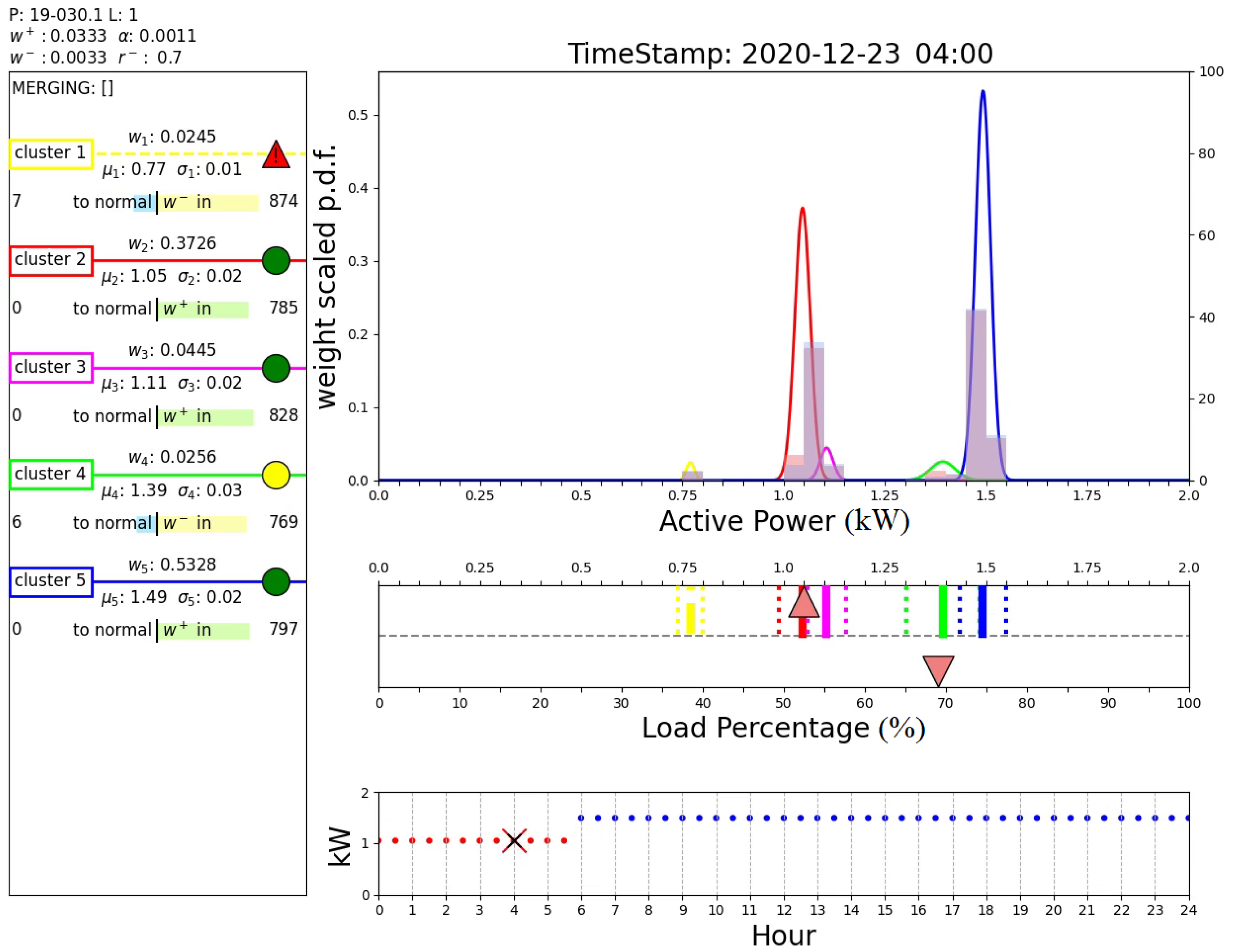
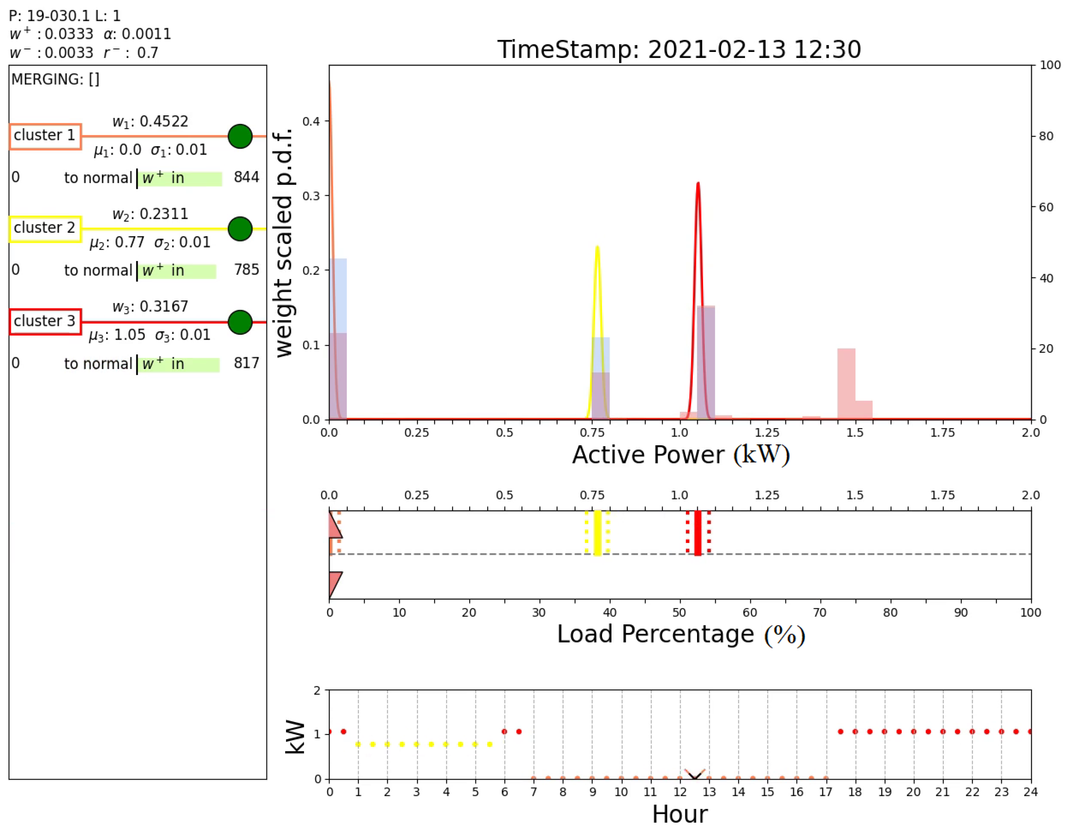
Figure 12 shows the output of the proposed algorithm at 31 d 6 h 30 min of the time series. Above box A, the plant identification number and the values of the main parameters of the algorithm are reported. Box A summarizes the parameters of all the active clusters (weight, mean, and standard deviation). Additionally, for each cluster the number of consecutive samples required to normalize or to suppress the cluster is reported. Normal clusters are denoted with a continuous line and a green circle. Previously normalized clusters with a weight lower than are denoted with a continuous line and a yellow circle. Clusters which have never been normal are denoted with a dotted line and a red triangle. Box B reports the probability density functions with the related weights computed according to the proposed AutoGMM reported on the left y-axis. Additionally, two different histograms are shown, equivalent to the histogram reported in Figure 10. The red histogram is related to the whole data collected up to the current sample, while the blue histogram refers to data collected in the last 24 h. Box C reports the cluster distributions. For each cluster, the centered line denotes the cluster mean while the dotted lines delimit the inlier range of the cluster according to its standard deviation. The orange triangle in the upper part of the box denotes the active power of the current sample. The orange triangle in the lower part of the box represents the relative percentage power of the actual sample with respect to the maximum power ever registered. Finally, box D reports the active power predictions over a day provided by the DTree.
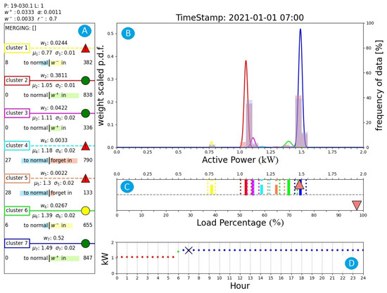
Figure 12.
Output of the proposed algorithm at 31 d 6 h 30 min (nominal operating condition). (A): active clusters and related parameters; (B): probability density functions and data frequency distribution; (C): cluster distributions; (D): clusters predicted by DTree.
The colors of the dots of the figure reported in this box depend on the color of the expected cluster, as in box A. The cross denotes the active power of the current sample. In this case, there are only three expected clusters and the current active power matches the predicted active power and no anomalies are claimed. Note also that even if cluster 3 is a normal cluster, it is not an expected cluster from the DTree.
Figure 13 shows the output of the proposed algorithm at 20 d 3 h 30 min, when an anomaly is detected. In fact, while the cluster predicted from the DTree is cluster 2, the active power of the current sample is significantly lower and belongs to cluster 1, which is not normal, i.e., it represents an abnormal operating condition. This figure clearly shows that the algorithm was able to detect the anomaly visible in Figure 11 at day 20.
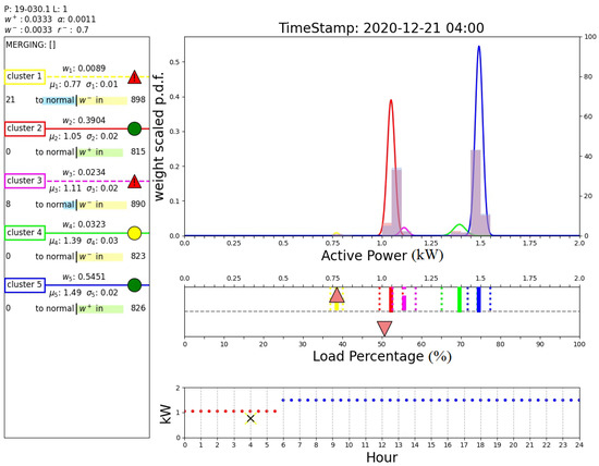
Figure 13.
Output of the proposed algorithm at 20 d 3 h 30 min (anomaly detection).
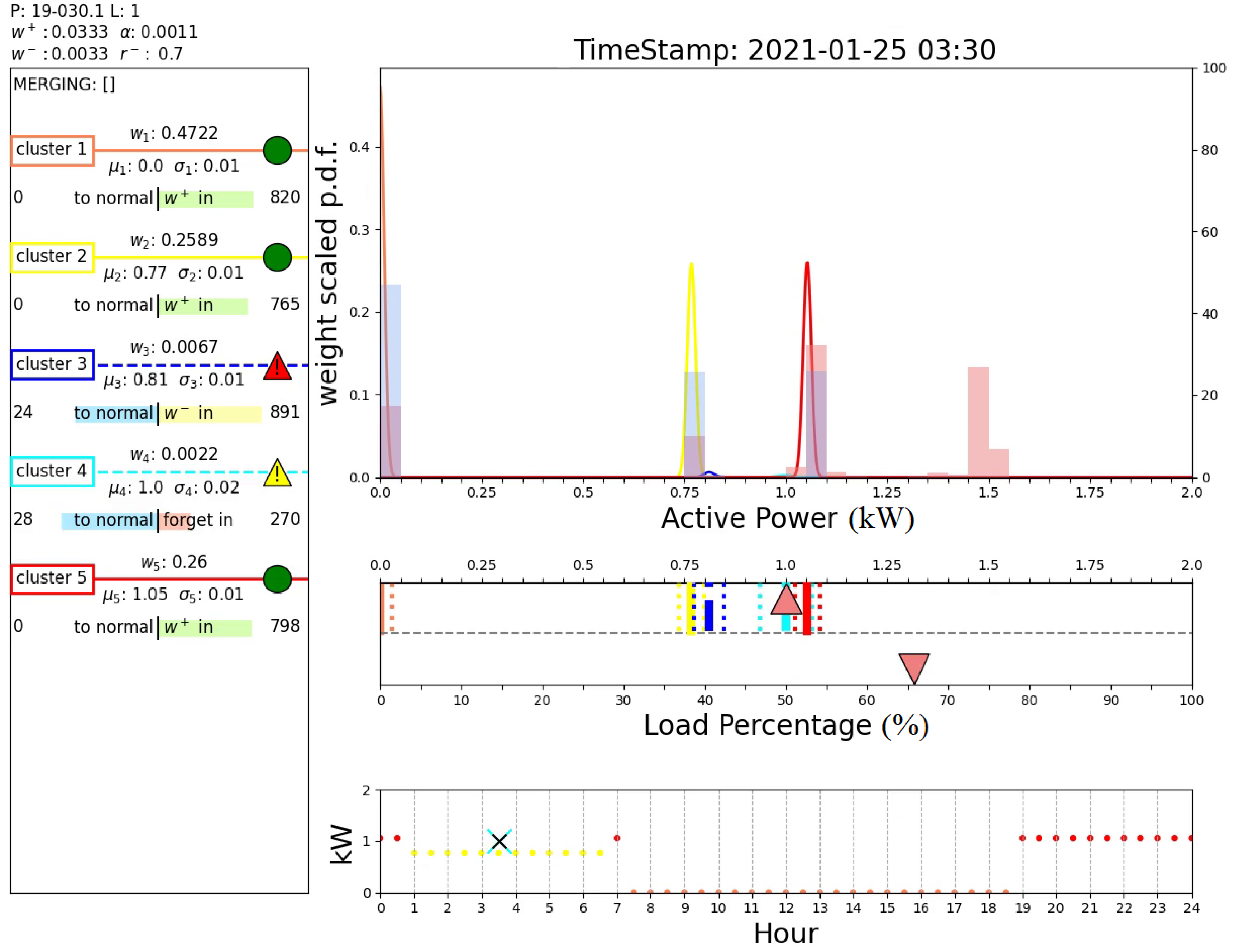
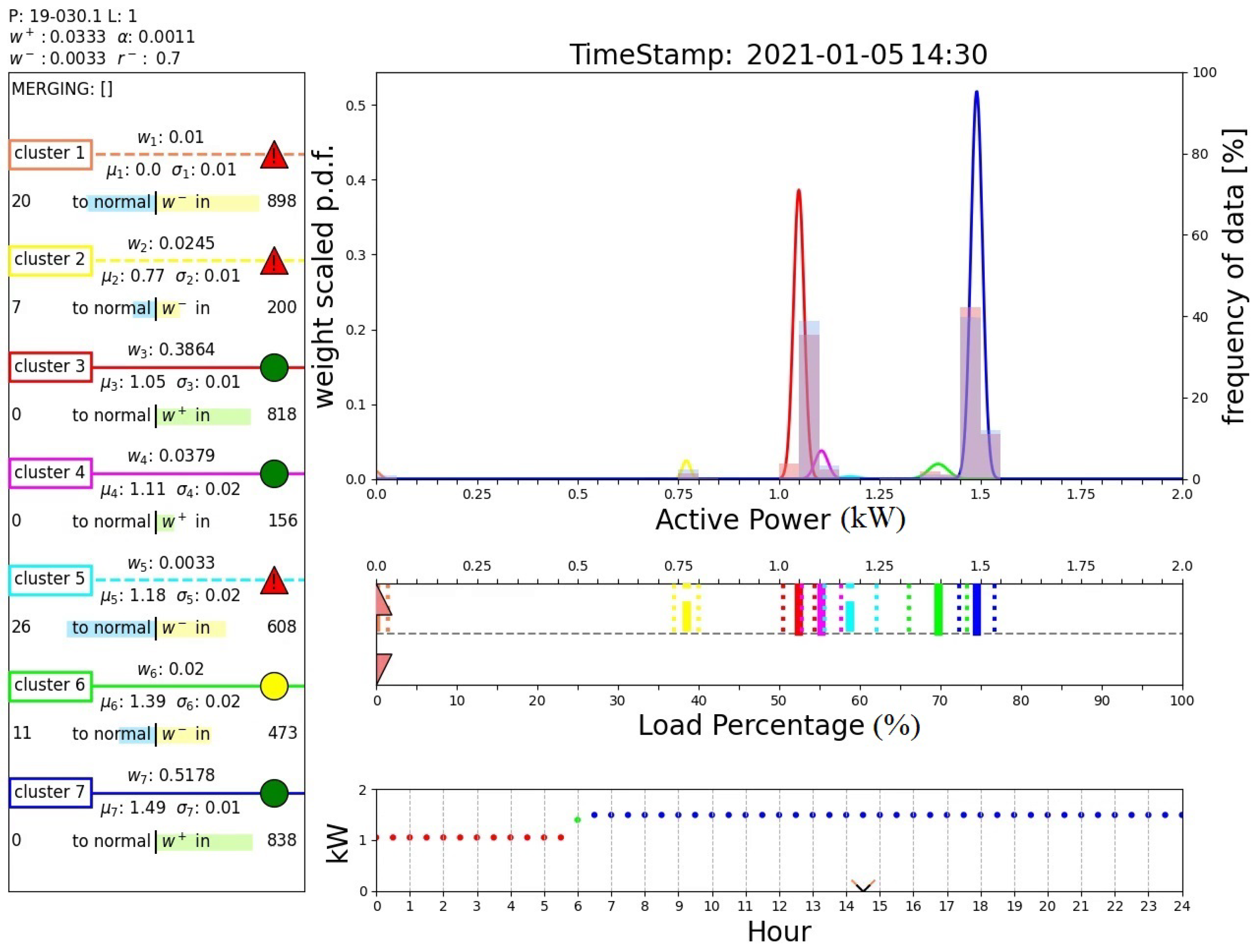
Figure 14 shows that two days after the detection of the anomaly, the faulty cluster is not considered as an expected operating mode by the DTree. In fact, the figure shows that at hour 4:00 the expected cluster is still cluster 2, and this prediction is correct according to the measured active power in this time instant. However, it can be noted that cluster 1 is still an active cluster and has not been removed from the algorithm. This figure demonstrates the effective combination of the AutoGMM with the DTree.
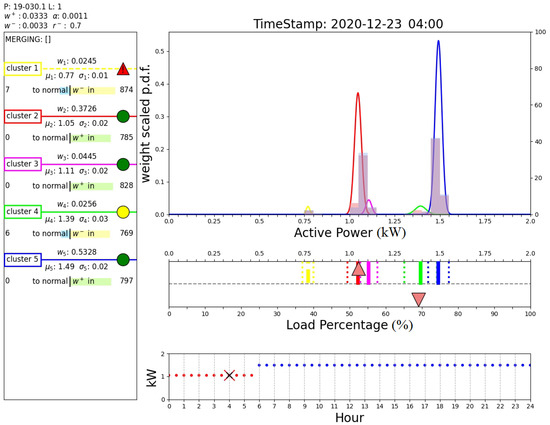
Figure 14.
Output of the proposed algorithm at 22 d 3 h 30 min.
Figure 15 shows the output of the proposed algorithm at 55 d 3 h 0 min, when another anomaly is detected. In fact, the cluster predicted from the DTree is cluster 5, while the active power of the current sample is higher and belongs to cluster 4. This demonstrates that the proposed method was able to recognize the anomaly at day 55 shown in Figure 11. Figure 16 shows how after 19 days the faulty cluster 4 (cyan) in Figure 15 is definitely removed from the sets of active clusters since it has not reached the normalization threshold. This means that the sample collected at 55 d 3 h 0 min is symptomatic of an abnormal operating condition. This analysis demonstrates the ability of the proposed algorithm to detect anomalies in the plant.

Figure 15.
Output of the proposed algorithm at 55 d 03 h 0 min (anomaly detection).
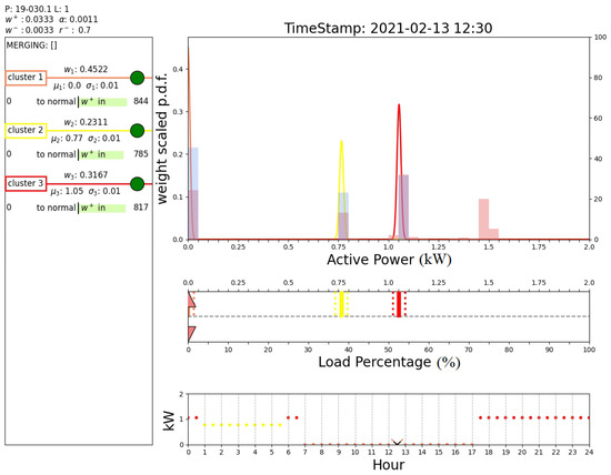
Figure 16.
Output of the proposed algorithm at 74 d 12 h 0 min (faulty cluster removal).
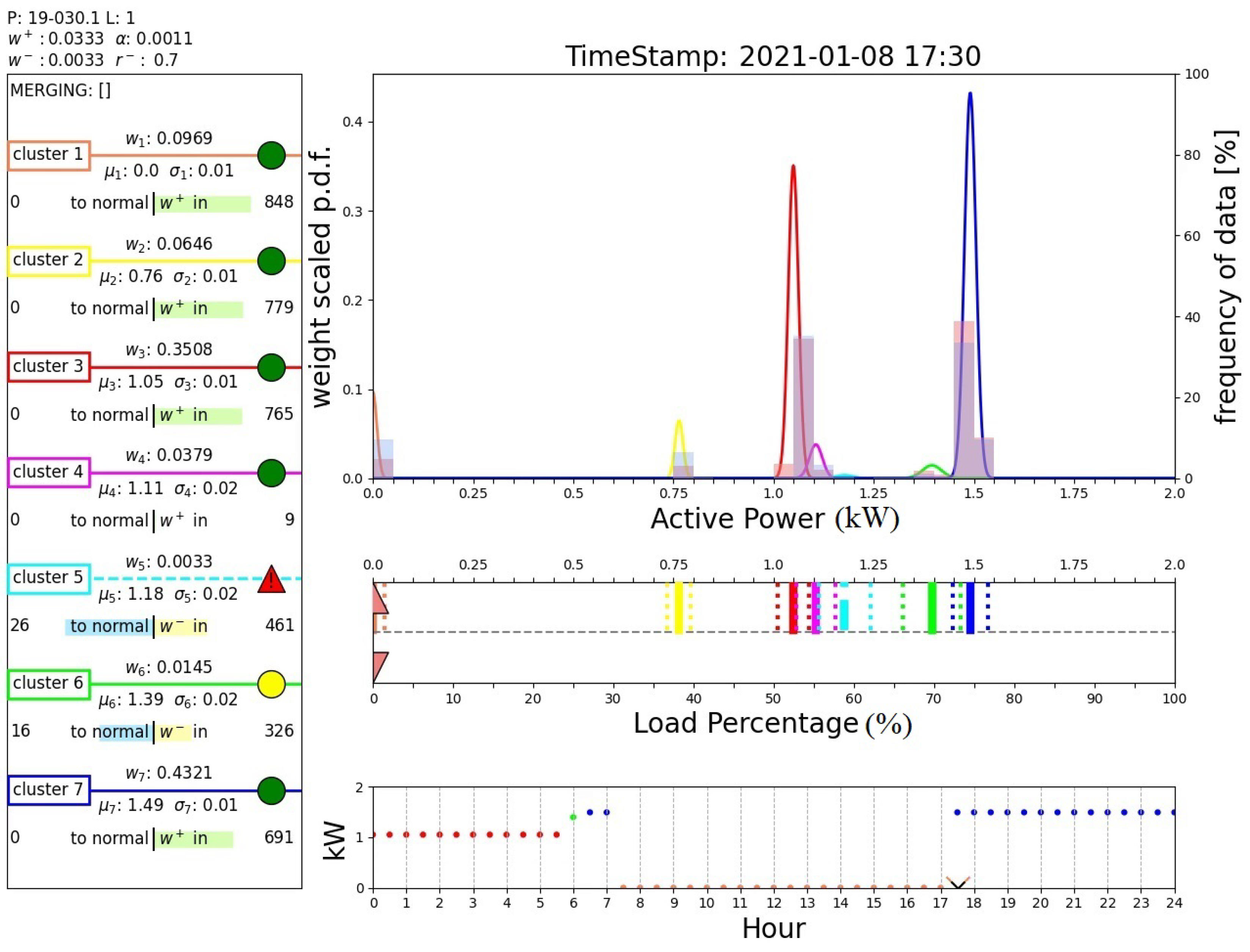
Finally, Figure 17 and Figure 18 report the outputs of the algorithm when a sample belonging to a new operating mode is detected. In fact, these two figures show the results obtained after day 36, when an abrupt variation in the operating modes is registered, as illustrated in Figure 11. Initially, the algorithm claims an anomaly of the system that is placed in a novel cluster (cluster 1, instead of the predicted cluster 7), as shown in Figure 17. Note that this cluster is associated with measurements around 0 kW, which are handled by the proposed algorithm as all the other power measurement values. Unlike the case shown in Figure 16, such a cluster is normalized and recognized as a new operating mode of the system; see box D of Figure 18. In fact, the DTree predicts cluster 1 as the expected cluster in the time range 7:30–18:30. This outcome demonstrates the ability of the proposed algorithm to perform novelty detection.
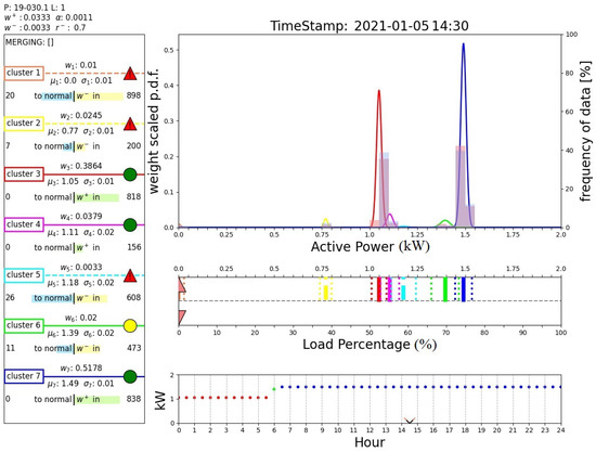
Figure 17.
Output of the proposed algorithm at 35 d 14 h 0 min (first, condition detected as anomaly).
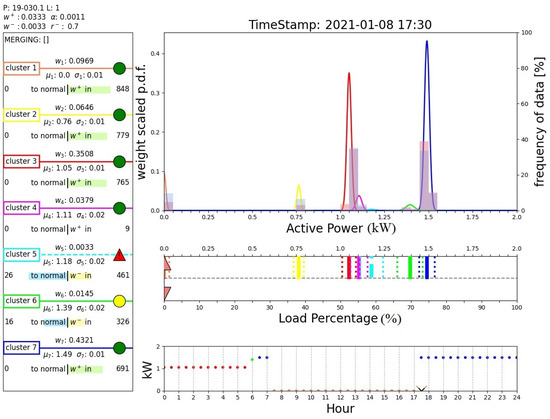
Figure 18.
Output of the proposed algorithm at 38 d 17 h 0 min (then, recognized as new operating condition).
5. Conclusions
This article has presented a novel online method, called AutoGMM-DTree algorithm, for the condition monitoring of electrical industrial loads. An automated Gaussian mixture model (AutoGMM) has been designed to group the active power measurements in clusters representative of the operating modes of the plant. Additionally, a decision tree (DTree) has been paired with the AutoGMM to predict normal operating conditions and detect anomalies. The method has been validated using data provided by a real industrial plant with a daily periodic power consumption by adopting a cloud-computing implementation. The results demonstrate the ability of the proposed method to automatically recognize regular operating modes of the plant, detect abnormal operating modes, and acknowledge new operating modes. As future work we plan to analyze the impact of hyperparameters on the performance of the proposed method (e.g., the learning rate of the AutoGMM and the parameters used by the cluster removal procedure) and its applicability/scalability to other industrial plants characterized by different power levels and periodic patterns.
Author Contributions
Conceptualization, G.L.C., D.C. and F.R.; methodology, D.C. and F.R.; software, D.C. and F.R.; validation, A.P.; formal analysis, P.S., D.C. and F.R.; investigation, P.S., D.C. and F.R.; resources, D.C. and F.R.; data curation, P.S., D.C. and F.R.; writing—original draft preparation, E.B., P.V. and M.T.; writing—review and editing, E.B., P.V. and M.T.; visualization, E.B. and P.V.; supervision, A.P. and G.L.C.; project administration, A.P.; funding acquisition, A.P. All authors have read and agreed to the published version of the manuscript.
Funding
This work was supported in part by the project “DIRAC—DIgital twins, aRtificial intelligence, distributed Analytics and Control in edge/cloud computing environment of industrial equipment for performance optimization and predictive maintenance”—POR Puglia (Italy) FESR 2014/2020—Regolamento regionale della Puglia per gli aiuti in esenzione n. 17 del 30 Settembre 2014—Titolo II, Capo 1 “Aiuti ai programmi di investimento delle grandi imprese”—Proposing Company: Free Energy Saving S.r.l.—Project Code: 5LCGQ14-Project Name: “Dirac Fes 2022”—CIFRA (Proposal Identifier): 158/DIR/2023/00520—Approved by Competitiveness Section Puglia, resolution no. 507 dated 28 June 2023; and in part by the project “Fondo di finanziamento della Ricerca di Sistema elettrico nazionale Piano Triennale 2019–2021—Bando b—progetto “InSITE—INtelligent energy management of Smartgrids based on IoT and edge/cloud Technologies”, riferimento Prog. CSEAB_00320”.
Data Availability Statement
Restrictions apply to the availability of these data. The data were obtained from Free Energy Saving srl and are available from the authors with the permission of Free Energy Saving S.r.l.
Conflicts of Interest
The authors declare no conflict of interest.
Abbreviations
The following abbreviations are used in this manuscript:
| CM | Condition monitoring |
| AutoGMM | Automated Gaussian mixture model |
| GMM | Gaussian mixture model |
| DTree | Decision tree |
| ML | Machine learning |
| NILM | Non-intrusive load monitoring |
References
- Yan, H.C.; Zhou, J.H.; Pang, C.K. Gaussian mixture model using semisupervised learning for probabilistic fault diagnosis under new data categories. IEEE Trans. Instrum. Meas. 2017, 66, 723–733. [Google Scholar] [CrossRef]
- Zhao, Y.; Liu, Q.; Li, D.; Kang, D.; Lv, Q.; Shang, L. Hierarchical anomaly detection and multimodal classification in large-scale photovoltaic systems. IEEE Trans. Sustain. Energy 2018, 10, 1351–1361. [Google Scholar] [CrossRef]
- Nandi, S.; Toliyat, H.A.; Li, X. Condition monitoring and fault diagnosis of electrical motors—A review. IEEE Trans. Energy Convers. 2005, 20, 719–729. [Google Scholar] [CrossRef]
- Lee, J.; Wu, F.; Zhao, W.; Ghaffari, M.; Liao, L.; Siegel, D. Prognostics and health management design for rotary machinery systems—Reviews, methodology and applications. Mech. Syst. Signal Process. 2014, 42, 314–334. [Google Scholar] [CrossRef]
- Tipaldi, M.; Iervolino, R.; Massenio, P.R. Reinforcement learning in spacecraft control applications: Advances, prospects, and challenges. Annu. Rev. Control 2022, 54, 1–23. [Google Scholar] [CrossRef]
- Martínez, J.C.; Gonzalez-Longatt, F.; Amenedo, J.L.R.; Tricarico, G. Cyber-physical Framework for System Frequency Response using Real-time simulation Phasor Measurement Unit based on ANSI C37.118. In Proceedings of the IEEE Power & Energy Society General Meeting (PESGM), Orlando, FL, USA, 25 September 2023; pp. 1–5. [Google Scholar]
- Zinoviev, G.; Udovichenko, A. The calculating program method of the integrated indicator of grid electromagnetic compatibility with consumers combination of non-sinusoidal currents. In Proceedings of the International Multi-Conference on Engineering, Computer and Information Sciences (SIBIRCON), Novosibirsk, Russia, 18–22 September 2017; pp. 481–484. [Google Scholar]
- Qureshi, M.; Ghiaus, C.; Ahmad, N. A blind event-based learning algorithm for non-intrusive load disaggregation. Int. J. Electr. Power Energy Syst. 2021, 129, 106834. [Google Scholar] [CrossRef]
- Hiruta, T.; Maki, K.; Kato, T.; Umeda, Y. Unsupervised learning based diagnosis model for anomaly detection of motor bearing with current data. Procedia CIRP 2021, 98, 336–341. [Google Scholar] [CrossRef]
- Qiu, Z.; Yuan, X.; Wang, D.; Siwen, F.; Wang, Q. Physical model driven fault diagnosis method for shield Machine hydraulic system. Measurement 2023, 220, 113436. [Google Scholar] [CrossRef]
- Jiang, L.; Sheng, H.; Yang, T.; Tang, H.; Li, X.; Gao, L. A New Strategy for Bearing Health Assessment with a Dynamic Interval Prediction Model. Sensors 2023, 18, 7696. [Google Scholar] [CrossRef]
- Brescia, E.; Massenio, P.R.; Di Nardo, M.; Cascella, G.L.; Gerada, C.; Cupertino, F. Nonintrusive Parameter Identification of IoT-Embedded Isotropic PMSM Drives. IEEE J. Emerg. Sel. Top. Power Electron. 2023, 11, 5195–5207. [Google Scholar] [CrossRef]
- Brescia, E.; Massenio, P.R.; Di Nardo, M.; Cascella, G.L.; Gerada, C.; Cupertino, F. Parameter Estimation of Isotropic PMSMs Based on Multiple Steady-State Measurements Collected During Regular Operations. IEEE Trans. Energy Convers. 2023, 1–16. [Google Scholar] [CrossRef]
- Afridi, Y.S.; Hasan, L.; Ullah, R.; Ahmad, Z.; Kim, J.M. LSTM-Based Condition Monitoring and Fault Prognostics of Rolling Element Bearings Using Raw Vibrational Data. Machines 2023, 11, 531. [Google Scholar] [CrossRef]
- Zoha, A.; Gluhak, A.; Imran, M.A.; Rajasegarar, S. Non-intrusive load monitoring approaches for disaggregated energy sensing: A survey. Sensors 2012, 12, 16838–16866. [Google Scholar] [CrossRef] [PubMed]
- Surucu, O.; Gadsden, S.A.; Yawney, J. Condition Monitoring using Machine Learning: A Review of Theory. Expert Syst. Appl. 2023, 221, 119738. [Google Scholar] [CrossRef]
- Massenio, P.R.; Rizzello, G.; Naso, D.; Yawney, J. Fuzzy Adaptive Dynamic Programming Minimum Energy Control Of Dielectric Elastomer Actuators. In Proceedings of the IEEE International Conference on Fuzzy Systems (FUZZ-IEEE), New Orleans, LA, USA, 23–26 June 2019; pp. 1–6. [Google Scholar]
- Himeur, Y.; Ghanem, K.; Alsalemi, A.; Bensaali, F.; Amira, A. Artificial intelligence based anomaly detection of energy consumption in buildings: A review, current trends and new perspectives. Appl. Energy 2021, 287, 116601. [Google Scholar] [CrossRef]
- Pan, H.; Yin, Z.; Jiang, X. High-dimensional energy consumption anomaly detection: A deep learning-based method for detecting anomalies. Energies 2022, 15, 6139. [Google Scholar] [CrossRef]
- Widodo, A.; Yang, B.S. Support vector machine in machine condition monitoring and fault diagnosis. Mech. Syst. Signal Process. 2007, 21, 2560–2574. [Google Scholar] [CrossRef]
- Ao, S.I.; Gelman, L.; Karimi, H.R.; Tiboni, M. Advances in Machine Learning for Sensing and Condition Monitoring. Appl. Sci. 2022, 12, 12392. [Google Scholar] [CrossRef]
- Yu, G.; Li, C.; Sun, J. Machine fault diagnosis based on Gaussian mixture model and its application. Int. J. Adv. Manuf. Technol. 2010, 48, 205–212. [Google Scholar] [CrossRef]
- Javed, M.R.; Shabbir, Z.; Asghar, F.; Amjad, W.; Mahmood, F.; Khan, M.O.; Virk, U.S.; Waleed, A.; Haider, Z.M. An Efficient Fault Detection Method for Induction Motors Using Thermal Imaging and Machine Vision. Sustainability 2022, 14, 9060. [Google Scholar] [CrossRef]
- Zhang, J.; Zhang, H.; Ding, S.; Zhang, X. Power consumption predicting and anomaly detection based on transformer and K-means. Front. Energy Res. 2021, 9, 779587. [Google Scholar] [CrossRef]
- Zivkovic, Z. Improved adaptive Gaussian mixture model for background subtraction. In Proceedings of the 17th International Conference on Pattern Recognition, Cambridge, UK, 23–26 August 2004; Volume 2, pp. 28–31. [Google Scholar]
- Chaleshtori, A.E.; Aghaie, A. A novel bearing fault diagnosis approach using the Gaussian mixture model and the weighted principal component analysis. Reliab. Eng. Syst. Saf. 2024, 242, 109720. [Google Scholar] [CrossRef]
- Costa, V.G.; Pedreira, C. Recent advances in decision trees: An updated survey. Artif. Intell. Rev. 2023, 56, 4765–4800. [Google Scholar] [CrossRef]
- Shivahare, B.D.; Suman, S.; Challapalli, S.S.N.; Kaushik, P.; Gupta, A.D.; Bibhu, V. Survey Paper: Comparative Study of Machine Learning Techniques and its Recent Applications. In Proceedings of the 2022 2nd International Conference on Innovative Practices in Technology and Management (ICIPTM), Gautam Buddha Nagar, India, 23–25 February 2022; pp. 449–454. [Google Scholar]
- Adams, S.; Beling, P.A. A survey of feature selection methods for Gaussian mixture models and hidden Markov models. Artif. Intell. Rev. 2019, 52, 1739–1779. [Google Scholar] [CrossRef]
- Seeja, G.; Doss, A.S.A.; Hency, V.B. A Novel Approach for Disaster Victim Detection Under Debris Environments Using Decision Tree Algorithms With Deep Learning Features. IEEE Access 2023, 11, 54760–54772. [Google Scholar] [CrossRef]
- Ming, D.; Zhu, Y.; Qi, H.; Wan, B.; Hu, Y.; Luk, K.D.K. Study on EEG-based mouse system by using brain-computer interface. In Proceedings of the IEEE International Conference on Virtual Environments, Human-Computer Interfaces and Measurements Systems, Hong Kong, China, 11–13 May 2009; pp. 236–239. [Google Scholar]


Disclaimer/Publisher’s Note: The statements, opinions and data contained in all publications are solely those of the individual author(s) and contributor(s) and not of MDPI and/or the editor(s). MDPI and/or the editor(s) disclaim responsibility for any injury to people or property resulting from any ideas, methods, instructions or products referred to in the content. |
© 2023 by the authors. Licensee MDPI, Basel, Switzerland. This article is an open access article distributed under the terms and conditions of the Creative Commons Attribution (CC BY) license (https://creativecommons.org/licenses/by/4.0/).