Dimensional Optimization of a Modular Robot Manipulator

Abstract

The mechanism parameters of the manipulator not only have a great influence on the size of the working space but also affect flexible performance distribution. Aimed at obtaining a 6 DOF modular manipulator, mechanism parameters were optimized in order to explore the effect of upper arm and forearm dimensions on the end dexterity of the manipulator. First, forward kinematic equations were derived using the DH method, and the Jacobian matrix of the manipulator was solved. Second, three indicators, including the condition number index, structural length index, and global conditioning index, were employed as optimization indicators for the mechanism parameters of the manipulator, and an orthogonal experiment was designed based on the Grey–Taguchi method and robot toolbox. Third, the grey relational analysis method was used to process the experimental results, and the grey relational grade for each group was solved. Last, the variation curve between the grey relational grade and the parameter level of each mechanism was drawn, and optimized mechanical arm mechanism parameters were derived. It was found that although the overall dimension of the manipulator was slightly decreased, as determined via comparing the original and optimized manipulator length, the performance indexes were improved. The results not only verified the correctness of the proposed optimization method but also laid a foundation for subsequent research on the dynamic performance of modular robot systems.

1. Introduction

A modular manipulator consists of a series of modules, such as links, joints and actuators, which have different functional size characteristics and certain assembly relationships. Each module can be connected electrically and mechanically to form a robotic arm structure with different workspaces and degrees of freedom [1]. The mechanism parameters of the manipulator not only have a great influence on the size of the working space but also affect flexible performance distribution. Therefore, it is very important to determine the optimal mechanism parameters of the manipulator in order to meet the requirements of the flexible performance of the manipulator in the design phase of the manipulator. The kinematics flexibility of manipulators is an element of key research content in robot kinematics. Many researchers at home and abroad have conducted research on robot kinematics and proposed many flexibility indexes, including the local performance index and global performance index. The local performance index includes measures of manipulability, the condition number, minimum singular value, motor dexterity index, etc. Global performance indexes include the SLI (structural length index), GMI (global manipulability index), GCI (global conditioning index), etc. [2]. Based on the flexibility index of the manipulator, many researchers at home and abroad have studied the parameter optimization of the manipulator mechanism. Xu et al. [3] considered multiple performance indexes such as dexterity and end stiffness and presented a method on how to maximally improve the comprehensive motion performance of anthropomorphic manipulators via optimizing link lengths. After optimization, the global comprehensive performance index value of the manipulator increased by about 23.97%, and motion performance was significantly improved. Zhao et al. [4] used manipulator manipulability as an optimization objective to optimize the size parameters of the connecting rod of the abdominal minimally invasive surgery robot. After optimization, the overall flexibility of the robot was improved. Hwang et al. [5] optimized the link length parameters of 7 DOF (degree of freedom) manipulators with the genetic algorithm by using the SLI (structural length index), GCI (global conditioning index), and MDCI (modified dynamic conditioning index) as the design indexes. Hyeon-Guk Kim et al. [6] proposed a method based on the condition number, SLI, and GCI to determine the size of the manipulator link and applied this method to optimize and analyze the 7 DOF manipulator and finally obtain the optimal size of the arm link. Mohd Zaman et al. [7] used an artificial bee colony algorithm (ABC) to optimize the structural dimensions of a 4 DOF robot manipulator. It was found that the robot manipulator with optimized dimensions effectively reaches the desired end-effector position and with less error. Zhang et al. [8] proposed four kinds of new indicators based on manipulability, condition number, and the minimum singular value, which were used to optimize the performance analysis and structure size of the manipulator. Taking the 2 DOF manipulator as an example, the structure of the manipulator was optimized, and the optimized link size was obtained. Gao et al. [9] proposed an optimized design method that can change the combination mode and order of each module and verified it with an example. Ma et al. [10] constructed the comprehensive dexterity evaluation indicator based on the condition number and measure of manipulability to optimize the parameters of the manipulator link. Finally, it made the manipulator have good isotropy and a good manipulability measure. Allaoua et al. [11], based on the LSI (local sensitivity index), proposed a new dimensionless sensitivity metric and used it to identify critical errors to reduce the geometric errors of the robot.

This paper focuses on the modular arm of a service robot developed by the research group (Shanghai University). In order to meet the requirements of the experiment, one DOF is added to the original 5 DOF manipulator, and the length of the big arm and the small arm of the manipulator are unequal. Previous research [12,13] shows that when the size of the big arm and the size of the small arm are equal, the flexibility of the end is the maximum. In order to investigate the influence of the size of the big arm and the small arm on its terminal flexibility, the structural parameters of the manipulator are optimized based on the flexible performance index.

The optimized robotic arm can be used in the field of home service robots and medical assistive robots because these robots need smaller arm sizes and greater flexibility to meet job requirements.

In this paper, the Grey–Taguchi method was mainly used to design orthogonal experiments thereby optimizing the link length of the robotic arm. Previous studies have verified [14] that this method not only has a small workload but also has a very uniform distribution of data points and is highly representative.

Section 2 of this paper briefly introduces the composition of the manipulator used in this study and presents a kinematic analysis. Section 3 introduces the basic concepts of the evaluation indicators SLI, GCI, and Cv that were used in this study. Section 4 introduces the design of orthogonal experiments based on the Grey–Taguchi method. Section 5 presents the results of the experiment. Section 6 analyzes the optimization results. Finally, Section 7 gives the conclusion.

2. Kinematic Analysis of Manipulator

2.1. Manipulator Model

The modular manipulator studied in this paper was manufactured by the Power Cube module of the German Amtec company. In this paper, we discuss a modular arm that was equipped on a mobile robot. The construction process of the whole robot system is shown in Figure 1. In the upper left corner of Figure 1 are six motor modules and one hand claw module, while in the lower left corner are seven connecting parts for connecting the motor module, hand claw module, and robot body. The connecting parts between each module were designed and fabricated by the research group. The robotic arm in the middle of Figure 1 was composed of these modules and connecting parts.

According to the mechanism structure, the modified DH method [15] was used to establish the kinematic scheme of the manipulator as shown in Figure 2, and the DH parameters of the manipulator are shown in

Table 1. DH parameter of the manipulator.

Joints	${\mathit{\theta }}_{\mathit{i}}\mathbf{/}\mathbf{(}°\mathbf{)}$	${\mathit{\alpha }}_{\mathit{i}\mathbf{-}\mathbf{1}}\mathbf{/}\mathbf{(}°\mathbf{)}$	${\mathit{a}}_{\mathit{i}-\mathbf{1}}\mathbf{/}\mathbf{\left(}\mathit{m}\mathbf{\right)}$	${\mathit{d}}_{\mathit{i}}\mathbf{/}\mathbf{\left(}\mathit{m}\mathbf{\right)}$	Range of Joints
1	${\theta }_1$	0	0	0	−180~180
2	${\theta }_2$	−90	0	$d_2$	−180~180
3	${\theta }_3$	90	0	0	−120~120
4	${\theta }_4$	−90	0	$d_4$	−180~180
5	${\theta }_5$	90	0	0	−120~120
6	${\theta }_6$	−90	0	$d_6$	−180~120

In which $d_2=0.328 \mathrm{m},d_4=0.2765 \mathrm{m},d_6=0.3362 \mathrm{m}$.

.

2.2. Kinematics Analysis

According to the DH parameters in Table 1, the kinematics equation of the manipulator can be obtained by using the transformation formula between the links of the manipulator link. The coordinate transformation matrix of the end-actuator of the manipulator to the basis coordinate system is as follows:

$$\begin{gathered} T_6^0\left(\theta \right)=\prod _{i=1}^6\left(T_i^{i-1}\left({\theta }_i\right)\right)=T_1^0{T}_2^1{T}_3^2{T}_4^3{T}_5^4{T}_6^5 \\ =\left[\begin{array}{cc}n& o\\ 0& 0\end{array}\begin{array}{cc}a& p\\ 0& 1\end{array}\right]=\left[\begin{array}{c}{n}_x\\ n_y\\ n_z\\ 0\end{array}\begin{array}{c}{o}_x\\ o_y\\ o_z\\ 0\end{array}\begin{array}{c}{a}_x\\ a_y\\ a_z\\ 0\end{array}\begin{array}{c}{p}_x\\ p_y\\ p_z\\ 1\end{array}\right] \end{gathered}$$

(1)

where ${\theta }_i$ denotes the joint angle, $p={\left[p_x{p}_y{p}_z\right]}^T$ means the position matrix, and $R=\left[noa\right]$ is the attitude matrix.

2.3. Jacobian Matrix

The linear transformation of the operating speed and joint velocity of the manipulator is defined as the Jacobian matrix of the manipulator. It can be seen as the transmission ratio from joint space to operation space. It is divided into geometric Jacobian and analytical Jacobian, which are not equal and have different meanings [16]. In this paper, the geometric Jacobian matrix of the manipulator was solved. Its calculation formula is as follows:

$$J=\left[\begin{array}{c}{J}_{Pn}\\ J_{On}\end{array}\right]=\left[\begin{array}{c}{z}_o\times (P_n-P_o)\\ z_0\end{array}\begin{array}{c}\cdots \\ \cdots \end{array}\begin{array}{c}{z}_{n-1}\times (P_n-P_{n-1})\\ z_{n-1}\end{array}\right]$$

(2)

$$z_{n-1}=R_1^0({\theta }_1)R_2^1({\theta }_2)\cdots R_{n-1}^{n-2}{(\theta }_{n-1})z_0$$

(3)

$$P_n=T_1^0({\theta }_1)T_2^1({\theta }_2)\cdots T_{n-1}^{n-2}{(\theta }_n)P_0$$

(4)

where $z_0={\left[0,0,1\right]}^T$ and $P_0={\left[0,0,0,1\right]}^T$. $z_{i-1}$ is the $z$-axis unit vector in the $i-1$ coordinate system, and $P_i$ is the position vector in the $n$ coordinate system, respectively. $R_i^{i-1}$ is the rotation matrix of the attitude of the link coordinate system.

3. Discrete Coefficient of Local and Global Index and Condition Numbers

There are many indicators to evaluate the flexibility of the motion of the manipulator; some local performance indexes, including operability, condition number, and global performance indexes, including SLI and GCI, are mentioned in [2]. And many other evaluation indexes, such as operation degree, redundancy index, and so on, are discussed in [2]. The condition number can reflect the stability and control accuracy of the kinematic solution of the robotic arm, help the designer evaluate the performance of the robotic arm, and provide a basis for the selection of control strategies and trajectory generation. SLI can be used to determine the link length of a manipulator to improve motion efficiency. GCI is used to evaluate the motion flexibility and stability of a manipulator at different workspace positions and orientations. In this paper, the condition number, SLI, and GCI were applied in [2].

3.1. Condition Number Index

The condition number of the Jacobian matrix was first proposed by Salisbury et al. as a performance index related to the manipulator kinematics as an evaluation of manipulator kinematics [17]. The relation between the condition number and the Jacobian singular value is

$$\kappa \left(J\right)=\frac{{\sigma }_{max}(J)}{{\sigma }_{min}(J)}$$

(5)

where ${\sigma }_{max}(J)$ and ${\sigma }_{min}(J)$ are the maximum and minimum singular values of the Jacobian matrix.

It is difficult to calculate the conditional number of the Jacobian matrix with Equation (5). When the manipulator is in the singular position, the minimum singular value of the Jacobian matrix is 0. The condition number of Jacobi is infinitely large, which makes the calculation difficult. In order to resolve the problems of the condition number of the Jacobian matrix, the Euclidean norm of the condition number was chosen as the definition of the condition number. The calculation formula is as follows:

$$\kappa \left(J\right)=\sqrt{tr\left({JNJ}^T\right)tr(J^{-1}N{J}^{-T})}$$

(6)

$$N=\frac{1}{n}{I}_{n\times n}$$

(7)

where $tr()$ is the matrix trace, n is the dimensions of the Jacobian matrix, and I is the identity matrix.

When the value of the condition number is close to 1, the manipulator is farther from the singular configuration, and when it is equal to 1, the manipulator is in the isotropic configuration. When the value of the condition number is close to 0, the manipulator is located near the singular configuration, and the manipulator is in a singular configuration when the condition number is equal to 0.

3.2. SLI Index

The design of a manipulator aims to maximize the workspace at the end of the manipulator as a larger workspace allows for more flexibility in performing tasks. Generally, the longer the size of the manipulator is, the larger the workspace can be. However, if the configurations and link length distributions of mechanical arms of the same length are different, there can be significant differences in the workspace reachability. Therefore, in the design stage of the manipulator, it is important to choose a configuration that offers better performance, with a larger workspace and a smaller total link length. In this paper, the SLI was used to evaluate the structural efficiency of the manipulator. The SLI is defined as the ratio of the manipulator link length sum to the cube root of the workspace volume. It is not related to the configuration of the manipulator, and the calculation formula is as follows:

$$Q=\frac{L}{\sqrt[3]{V}}$$

(8)

$$L=\sum _{i=1}^n(a_{i-1}+d_i)$$

(9)

where $V$ is the volume of reachable workspace, $L$ is the length sum of the manipulator link, $a_{i-1}$ is the link length, $d_i$ is the link offset, and $a_{i-1}$ and $d_i$ are the values of the D-H parameter table.

In the structure design of the manipulator, it is usually expected that the length of the link is as short as possible, and the larger the workspace, the better. Therefore, the smaller the L value, the greater the V value; that is, the smaller the Q value, the better the design of the manipulator. In order to obtain the workspace volume in the SLI index. Firstly, the Monte Carlo method [18,19] was used to obtain the workspace point cloud. Then the workspace was discredited by the grid. Finally, the volume of the reachable workspace was calculated by the number of grids containing the space point.

The process was as follows:

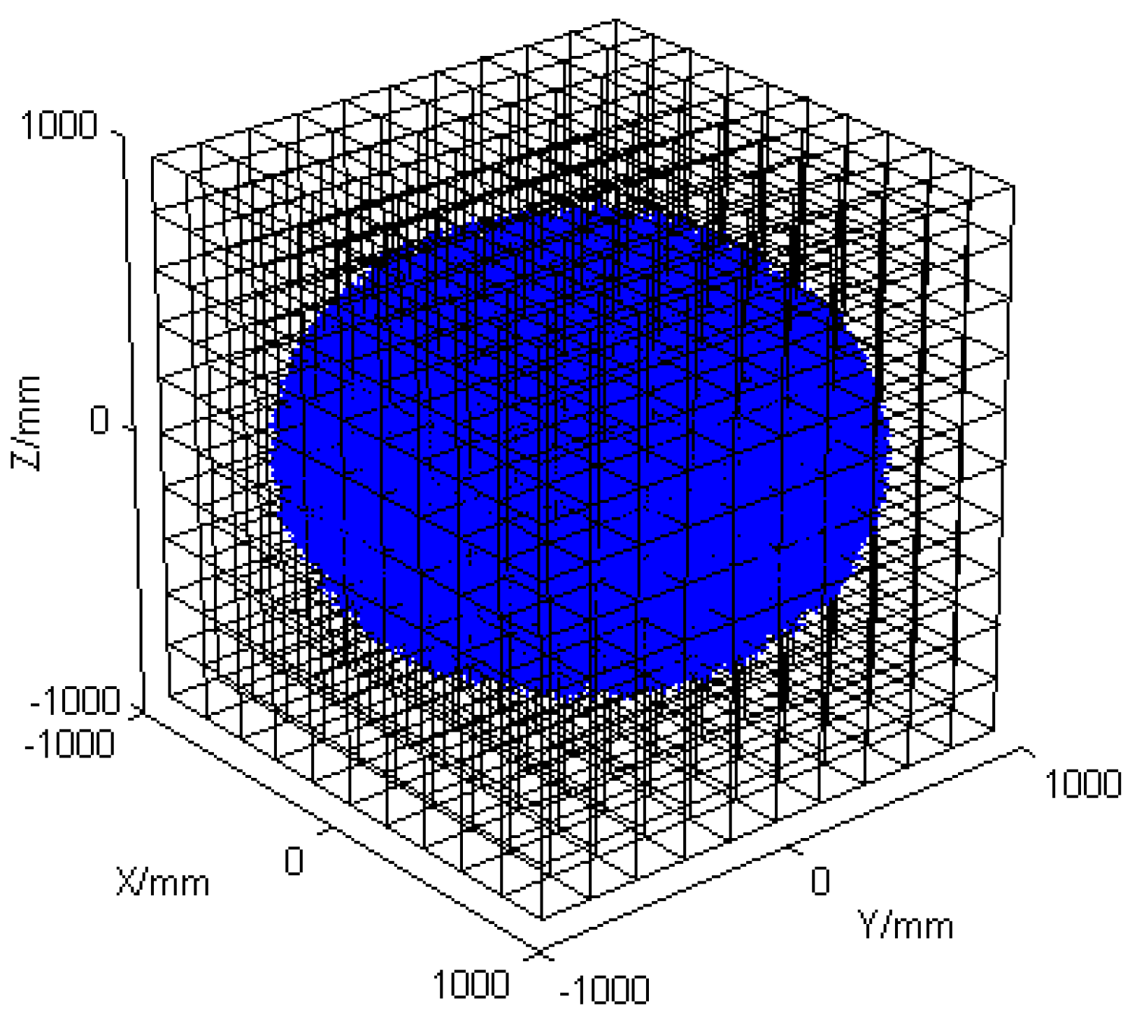
• In the MATLAB software environment of version 2021, the Robotics toolbox was used to build the model of the manipulator. The position coordinates of the end of the manipulator were obtained based on the Monte Carlo method and using the kinematics equation of the manipulator. Then the MATLAB visualization function was applied to display the position coordinates of these points by tracing them. The extent of the workspace point cloud and the projected limits of the workspace on each axis were obtained.
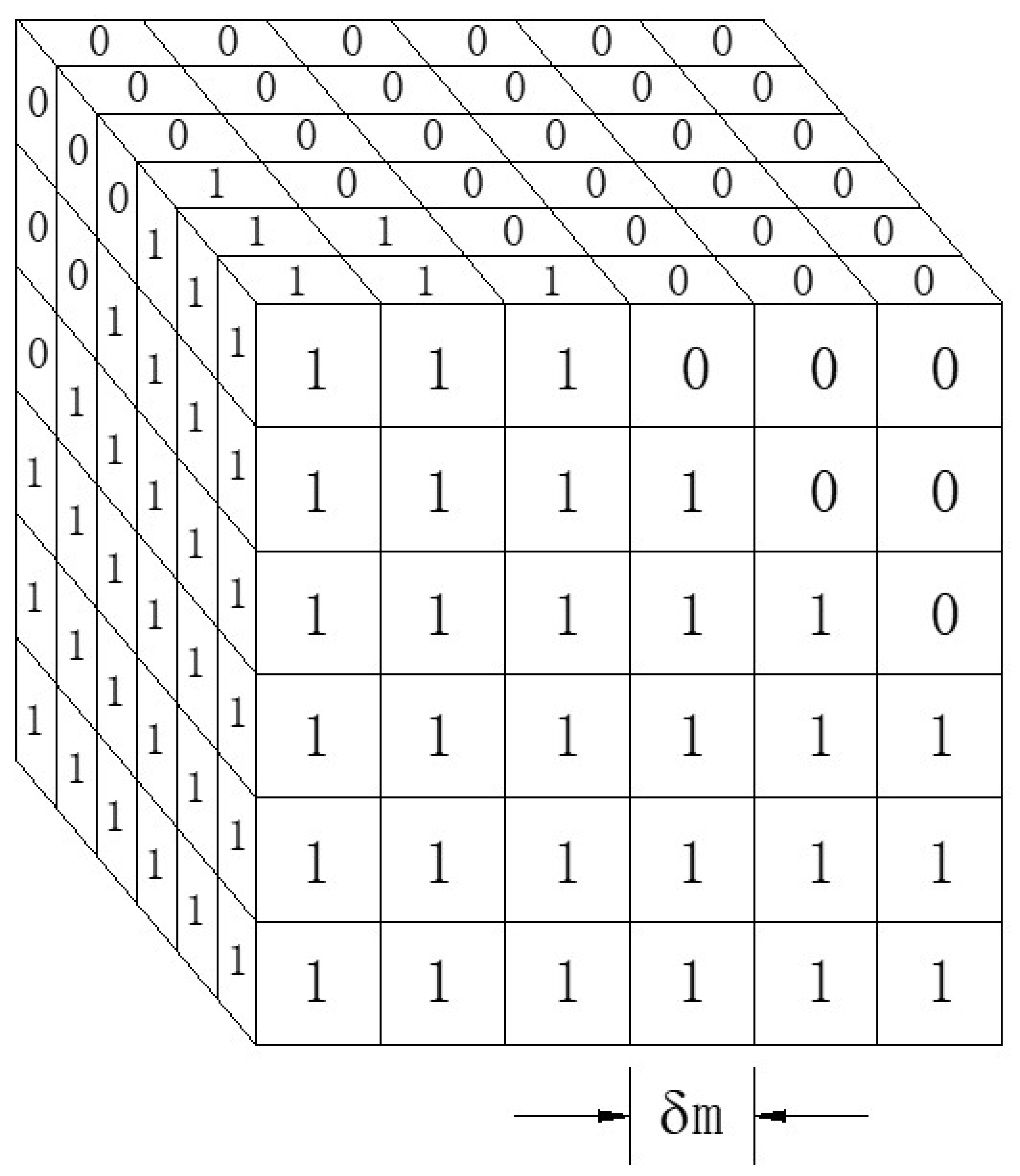
• A cube was formed by the maximum value of the limit of each coordinate axis in (1) as the edge length. The cube was used to envelop the manipulator to reach the workspace. The side length of the cube was divided into m parts, and the length of each section was $\mathsf{\delta }m$. The cube was divided into several small cubes, and each small cube had a value of ${(\mathsf{\delta }m)}^3$. The small cube could represent the end position of the manipulator and could be described with a 3D matrix [20]. Due to factors such as calculation time, the edge length of a small cube was taken as 2 mm in this paper. The reachable workspace point cloud and grid discretization processing are shown in Figure 3.
• The data of the end position of the manipulator were converted into a cube cell, which could be described by a 3D matrix. When the cube cell contained at least one position coordinate value, the 3D matrix that described the cell of the cube was assigned to 1, and the rest was assigned to 0. Its principle is shown in Figure 4.
• Finally, the workspace volume of the manipulator could be obtained by adding up the number of cube cells assigned to 1.

3.3. GCI

The GCI is a global performance index based on the Jacobian matrix condition number, which is not related to the manipulator configuration. Gosselin et al. [21] proposed that the GCI be used to analyze the distribution of condition numbers in the whole manipulator workspace. The index is defined as

$$\eta =\frac{A}{B}\in (0,1)$$

(10)

$$A={\int }_W(\frac{1}{\kappa })dW$$

(11)

$$B={\int }_{W}dW$$

(12)

where $\eta$ is the GCI, $W$ is a point of the manipulator workspace, $B$ is the workspace volume, and $\kappa$ is the condition number of the Jacobian matrix at the point. The $\eta$ ranges from

$$0<\eta <1$$

(13)

The workspace of the manipulator is not easily represented in Cartesian space, and Equations (11) and (12) are expressed in their joint space as

$$A={\int }_R(\frac{1}{\kappa })|\mathsf{\Delta }|d{\theta }_n\cdots d{\theta }_{2}d{\theta }_1$$

(14)

$$B={\int }_R|\mathsf{\Delta }|d{\theta }_{n}Ld{\theta }_{2}d{\theta }_1$$

(15)

where $R$ is the manipulator workspace in joint space and $\mathsf{\Delta }$ is the Jacobian matrix determinant.

Due to the fact that there is still a sixfold integral in the upper integral, the exact solution of the integral is not easy to solve, and the calculation process is more complicated. In this paper, the discrete equation was used to calculate and analyze, as follows:

$$\eta =\frac{1}{n_{WS}}\sum _{j=1}^{n_{WS}}\frac{1}{\kappa }$$

(16)

where $n_{WS}$ is the number of nodes in the manipulator workspace. Nodes refer to discrete points or locations within the workspace. Each node represents a specific location that the robotic arm can potentially reach.

Equation (10) indicates that the manipulator had better GCI performance when the GCI value was close to 1 and conversely the GCI performance was poor.

3.4. Discrete Coefficient of the Condition Number

The discrete coefficient is a statistical index in statistics that is mainly used to measure the degree of discretization of probability distribution data. Generally, the standard deviation is used to assess the dispersion of a dataset. The larger the average value of the general data is, the greater the standard deviation is. However, if the data contain different dimensions or units, they cannot be used to evaluate the degree of data dispersion. If the two groups are consistent and the mean and standard deviation are very different, the standard deviation is also no longer applicable. In the process of analyzing the two sets of data, if the average value of the two sets of data is equal, a set of data with a smaller standard deviation is generally selected, and if the standard deviation of the two sets of data is equal, a set of data with a better average is generally selected. However, when the two sets of data have different average values and standard deviations, the discrete coefficient is used to measure the pros and cons of the data. The calculation formula is

$$c_V=\frac{\sigma }{\mu }$$

(17)

where $c_V$ is the discrete coefficient, $\sigma$ is the standard deviation, and $\mu$ is the average value.

Equation (17) shows that the discrete coefficient is the standard deviation of the unit average value. It can be used to compare and analyze the data with different average values and standard deviations. The larger the discrete coefficient, the greater the degree of data dispersion.

4. Experiment Design

In the process of optimizing the parameters of the mechanism, different values were taken for the parameters of the different mechanisms, then they were arranged and combined, and finally, the optimal parameters of the mechanism were obtained. The calculation process was very complex and time-consuming, so it was necessary to design a suitable experiment for the problem of the optimization process mentioned above. The traditional experimental design methods include orthogonal array (OA), Latin hypercube design (LHD) [22], OA-based LHD, etc. In this paper, the Grey–Taguchi method [23,24] was used to design the orthogonal test, and the parameters of the manipulator mechanism were optimized. This method is suitable for optimization problems with multiple optimization objectives and has high prediction accuracy, strong interpretability, and less experimental computation. Optimization of the whole workspace can be time efficient compared with other optimization methods.

Orthogonal Experiment Design and Experiment Results

Orthogonal experimental design is a method that involves arranging experiments and analyzing the results using an orthogonal table. In this paper, three link lengths $(d_2,d_4,d_6)$ were used as design variables, so a three-factor five-level orthogonal experiment was designed for analysis, and the experiment was arranged according to the orthogonal table. Considering the influence of the size of the robot arm’s motor, reducer, and connectors, the mechanism was designed with five gradient levels by using the current mechanical parameters of the mechanical arm while avoiding interference of motion and not exceeding the maximum load of the motor. The highest level was 1.5 times the lowest level, and the five levels of link length data are shown in

Table 2. Five levels of the parameter of link size.

Link Number	Level 1 (m)	Level 2 (m)	Level 3 (m)	Level 4 (m)	Level 5 (m)
Link 1	0.2624	0.2952	0.328	0.3608	0.3936
Link 2	0.2212	0.2489	0.2765	0.3042	0.3318
Link 3	0.2690	0.3026	0.3362	0.3698	0.4034

In this table, the links 1, 2, and 3 correspond to $d_2,d_4$, and $d_6$, respectively.

.

5. Experiment Results Processing

5.1. Experiment Results

According to the dimensions of the three link lengths corresponding to the orthogonal experiment design method, the values of SLI, GCI and the discrete coefficient of the condition number are obtained. The results of the orthogonal experiment design and index calculation are shown in

Table 3. Orthogonal experimental design and the result of index values.

Group	Link 1	Link 2	Link 3	Cv	SLI	GCI
1	1 (0.2624)	1 (0.2212)	1 (0.2690)	94.4889	0.6856	0.0234
2	1 (0.2624)	2 (0.2489)	2 (0.3026)	94.5672	0.6787	0.0249
3	1 (0.2624)	3 (0.2765)	3 (0.3362)	94.6512	0.6732	0.0261
4	1 (0.2624)	4 (0.3042)	4 (0.3698)	94.7399	0.6686	0.0269
5	1 (0.2624)	5 (0.3318)	5 (0.4034)	94.8308	0.6648	0.0275
6	2 (0.2952)	1 (0.2212)	2 (0.3026)	94.5650	0.6889	0.0237
7	2 (0.2952)	2 (0.2489)	3 (0.3362)	94.6504	0.6821	0.0254
8	2 (0.2952)	3 (0.2765)	4 (0.3698)	94.7402	0.6765	0.0267
9	2 (0.2952)	4 (0.3042)	5 (0.4034)	94.8322	0.6719	0.0277
10	2 (0.2952)	5 (0.3318)	1 (0.2690)	94.5770	0.6805	0.0310
11	3 (0.3280)	1 (0.2212)	3 (0.3362)	94.6509	0.6918	0.0238
12	3 (0.3280)	2 (0.2489)	4 (0.3698)	94.7416	0.6850	0.0256
13	3 (0.3280)	3 (0.2765)	5 (0.4034)	94.8339	0.6795	0.0270
14	3 (0.3280)	4 (0.3042)	1 (0.2690)	94.5784	0.6899	0.0307
15	3 (0.3280)	5 (0.3318)	2 (0.3026)	94.6657	0.6835	0.0318
16	4 (0.3608)	1 (0.2212)	4 (0.3698)	94.7435	0.6943	0.0237
17	4 (0.3608)	2 (0.2489)	5 (0.4034)	94.8364	0.6877	0.0256
18	4 (0.3608)	3 (0.2765)	1 (0.2690)	94.5808	0.7002	0.0294
19	4 (0.3608)	4 (0.3042)	2 (0.3026)	94.6687	0.6925	0.0310
20	4 (0.3608)	5 (0.3318)	3 (0.3362)	94.7621	0.6862	0.0323
21	5 (0.3936)	1 (0.2212)	5 (0.4034)	94.8389	0.6966	0.0236
22	5 (0.3936)	2 (0.2489)	1 (0.2690)	94.5838	0.7120	0.0276
23	5 (0.3936)	3 (0.2765)	2 (0.3026)	94.6720	0.7023	0.0295
24	5 (0.3936)	4 (0.3042)	3 (0.3362)	94.7658	0.6948	0.0311
25	5 (0.3936)	5 (0.3318)	4 (0.3698)	94.8463	0.6886	0.0324

.

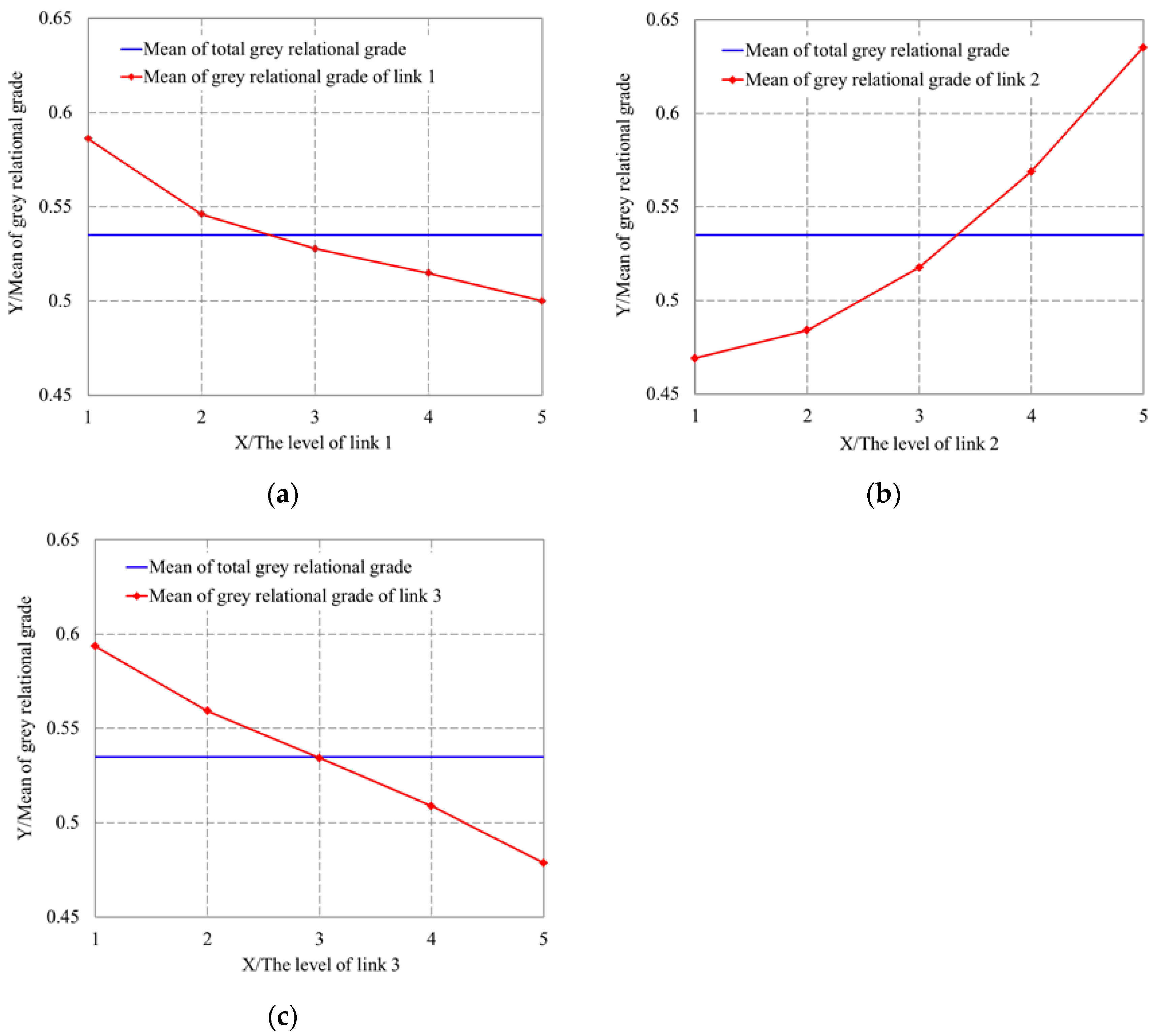
5.2. Grey Correlation Analysis of Experiment Results

In this paper, the grey relational analysis method [25,26,27] was used to process and analyze the experiment results. In order to facilitate the analysis, the calculated values of the above indicators must be processed. First, the index data in Table 3 were normalized. Next, the grey correlation coefficient was calculated based on the processed data to obtain the relationship between the actual data and the ideal value of the test. Finally, the correlation degree was calculated according to the grey correlation coefficient. However, the larger the index value of the above three indexes was, the smaller the value of the index was, so it needed to be calculated separately.

First, for the GCI, the larger the value was, the better the value was. The normalization is conducted by using Equation (18). For the SLI and the discrete coefficient of the condition number, the smaller the value was, the better the value was. Equation (19) was used for normalization. Where $x_o(k)=1$, the ideal value was 1. The final result is shown in

Table 4. Normalization data and grey relational coefficient results.

Group	Normalization Data			Grey Relational Coefficient
	Cv	SLI	GCI	Cv	SLI	GCI
1	1.0000	0.5593	0.0000	1.0000	0.5315	0.3333
2	0.7809	0.7055	0.1667	0.6953	0.6293	0.3750
3	0.5459	0.8220	0.3000	0.5241	0.7375	0.4167
4	0.2977	0.9195	0.3889	0.4159	0.8613	0.4500
5	0.0434	1.0000	0.4556	0.3433	1.0000	0.4787
6	0.7871	0.4894	0.0333	0.7014	0.4948	0.3409
7	0.5481	0.6335	0.2222	0.5253	0.5770	0.3913
8	0.2969	0.7521	0.3667	0.4156	0.6685	0.4412
9	0.0395	0.8496	0.4778	0.3423	0.7688	0.4891
10	0.7535	0.6674	0.8444	0.6698	0.6005	0.7627
11	0.5467	0.4280	0.0444	0.5245	0.4664	0.3435
12	0.2929	0.5720	0.2444	0.4142	0.5388	0.3982
13	0.0347	0.6886	0.4000	0.3412	0.6162	0.4545
14	0.7496	0.4682	0.8111	0.6663	0.4846	0.7258
15	0.5053	0.6038	0.9333	0.5027	0.5579	0.8823
16	0.2876	0.3750	0.0333	0.4124	0.4444	0.3409
17	0.0277	0.5148	0.2444	0.3396	0.5075	0.3982
18	0.7429	0.2500	0.6667	0.6604	0.4000	0.6000
19	0.4969	0.4131	0.8444	0.4985	0.4600	0.7627
20	0.2356	0.5466	0.9889	0.3954	0.5244	0.9783
21	0.0207	0.3263	0.0222	0.3380	0.4260	0.3383
22	0.7345	0.0000	0.4667	0.6532	0.3333	0.4839
23	0.4877	0.2055	0.6778	0.4939	0.3862	0.6081
24	0.2252	0.3644	0.8556	0.3922	0.4403	0.7759
25	0.0000	0.4958	1.0000	0.3333	0.4979	1.0000

.

$$x_i^{\prime }(k)=\frac{y_i\left(k\right)-min{y}_i(k)}{max{y}_i(k)-min{y}_i(k)}$$

(18)

$$x_i(k)=\frac{max{y}_i-y_i(k)}{max{y}_i(k)-min{y}_i(k)}$$

(19)

where $x_i^{\prime }\left(k\right)$ and $x_i(k)$ are the values of normalization, $y_i(k)$ is the $i$th experiment value of the indicator $k$, and $min{y}_i(k)$ and $max{y}_i(k)$ are the minimum and maximum values of the experiment value of the indicator $k$.

Second, the grey relational coefficient of each index was calculated. The grey relational coefficient reflects the relative difference between the data after processing and the ideal value. The calculation is given by Equations (20) and (21), and the calculation results are shown in Table 4.

$${\zeta }_i(k)=\frac{{\mathsf{\Delta }}_{min}+\zeta \times {\mathsf{\Delta }}_{max}}{{\mathsf{\Delta }}_{0i}(k)+\zeta \times {\mathsf{\Delta }}_{max}}$$

(20)

$${\mathsf{\Delta }}_{0i}=|x_0\left(k\right)-x_i(k)|$$

(21)

where $\zeta$ is the resolution coefficient, and the smaller $\zeta$ is, the better the resolution is (in which $\zeta =0.5$). ${\mathsf{\Delta }}_{min}$ and ${\mathsf{\Delta }}_{max}$ are the minimum and maximum values, respectively.

Finally, the grey relational grade of each group experiment was calculated by the data in Table 4 and sorted. The grey relational grade refers to the approximate degree of the experimental results of each group to the ideal results. The calculation formula is shown in Equation (22), and the final calculation results are shown in

Table 5. Grey relational grade and its order.

Group	Relational Grade	Order
1	0.6216	5
2	0.5665	10
3	0.5594	11
4	0.5757	8
5	0.6073	7
6	0.5124	15
7	0.4979	17
8	0.5084	16
9	0.5334	14
10	0.6777	1
11	0.4448	22
12	0.4504	21
13	0.4706	20
14	0.6256	4
15	0.6476	2
16	0.3992	24
17	0.4151	23
18	0.5535	12
19	0.5737	9
20	0.6327	3
21	0.3674	25
22	0.4901	19
23	0.4961	18
24	0.5361	13
25	0.6104	6

. The grey relationship grades of each group experiment are ranked in Table 5. The smaller the number, the higher the approximation between the experimental results and the ideal results.

$${\gamma }_i=\frac{1}{n}\sum _{k=1}^n{\zeta }_i(k)$$

(22)

where ${\gamma }_i$ is the grey relational grade in the $i$th experiment, and $n$ is the number of the performance index.

6. Optimization Result Analysis

According to the correlation degree data in Table 5, the average values of different levels of correlation degree of each mechanism parameter were calculated, and the results are shown in

Table 6. The mean of grey relational grade at each level and each link parameter.

Link Number	Level 1	Level 2	Level 3	Level 4	Level 5
Link 1	0.5861	0.5460	0.5278	0.5148	0.5000
Link 2	0.4691	0.4840	0.5176	0.5689	0.6351
Link 3	0.5935	0.5593	0.5342	0.5088	0.4788

. Corresponding curves are plotted according to the mean of grey relational grade in Table 6, as shown in Figure 5.

As can be seen in Table 5, the total mean value is 0.5349.

The optimized mechanism parameters should select the corresponding link length when the correlation degree is the highest. Figure 5 shows that level 1 of link 1, level 5 of link 2, and level 1 of link 3 had the largest mean grey relational grade in the corresponding link length. The parameters of the optimized and initial mechanism were compared as shown in

Table 7. Comparison of link size before and after optimization.

	Before Optimization (m)	After Optimization (m)
Link 1	0.3280	0.2624
Link 2	0.2765	0.3318
Link 3	0.3362	0.2690
Length of the arm	0.9407	0.8632

, and the optimization indexes of the manipulator before and after the optimization were compared as shown in

Table 8. Comparison of each optimizing index of the manipulator before and after optimization.

Index	Before Optimization	After Optimization	Percentage of Promotion (%)
Cv	94.6895	94.5554	1.40
SLI	0.6856	0.6742	1.66
GCI	0.0280	0.0293	4.64

.

It can be seen from Table 7 and Table 8 that the total length of the robot arm was reduced after optimization, but the conditional dispersion coefficient and the SLI and GCI of the manipulator were optimized by 1.40%, 1.66%, and 4.64%, respectively. This showed that the optimized manipulator mechanism parameters could make the manipulator have a better performance index than the initial one. In order to analyze the influence of each parameter on the optimization index and its order of primary and secondary, the experiment results were analyzed by variance analysis. This analysis shows which design variables had a significant impact on the objective function. The results are shown in

Table 9. Variance analysis results.

Link Parameter	Deviation Squared Sum	DOF	Mean Square Error	F Value	Square Sum Proportion
Link 1	0.0394	4	0.0099	58.7040	25.32%
Link 2	0.0921	4	0.0230	137.2161	59.19%
Link 3	0.0221	4	0.0055	32.8637	14.2%
Error	0.0020	12	[ ]	[ ]	1.29%
Sum total	0.1556	24	[ ]	[ ]	100%

.

It is known from the results in Table 9 that the sum of the deviation squared sum, mean square error, and F value [28] of link 2 were the largest among the three links mentioned above, indicating that the results of this experiment were most significantly affected by link 2. That is to say, link 2 had the greatest influence on the flexible performance index of the manipulator, followed by link 1 and link 3.

7. Conclusions

In this paper, the 6 DOF manipulator constructed by the group was taken as the research object to investigate the influence of the size of the big arm and the small arm on its terminal flexibility, and the structural parameters of the manipulator were optimized based on the flexible performance index. First, the kinematics equation of the manipulator was obtained, and the Jacobian matrix of the manipulator was solved. Second, the optimization indicator of mechanism parameters was a local index (condition number and the SLI) and global index (the GCI) for evaluating the flexible performance of the manipulator. Based on the Grey–Taguchi method, the above indexes were taken as the optimization target, and an orthogonal experiment was designed with the aid of the robotics toolbox. Finally, the grey relational analysis method was used to analyze the results of the experiment and calculate the grey relational degree of each experiment, and the optimized mechanism parameters were obtained when each performance index reached a better level.

The results obtained after optimization were as follows: the size of link 1 and link 3 was reduced, the size of link 2 was increased, and the total length of the robot arm was slightly reduced. The discrete coefficient of the condition number, SLI, and GCI of the optimized manipulator were increased by 1.4%, 1.66%, and 4.64%, respectively. According to the results of ANOVA, link 2 was the most important factor affecting the flexible performance of the manipulator, followed by link 1 and link 3. The experimental results showed that the dimensions of the large arm and the small arm tended to be the same length, and the flexibility of the end of the manipulator was improved. The maximum influence of link 2 on the flexibility was also in line with the principle of “move the small arm more, move the large arm less” when the manipulator was in motion. The experimental results verified the feasibility of the scheme in this paper. This paper provides a certain theoretical basis for the design of the manipulator and lays the foundation for the subsequent study of the dynamic performance of the manipulator and the optimization of dynamic parameters.

References

1. Gao, W.; Wang, H.; Jiang, Y.; Pan, X. Research on the Calibration for a Modular Robot. J. Mech. Eng. 2014, 50, 33–40. [Google Scholar] [CrossRef]
2. Patel, S.; Sobh, T. Manipulator Performance Measures—A Comprehensive Literature Survey. J. Intell. Robot. Syst. 2015, 77, 547–570. [Google Scholar] [CrossRef]
3. Xu, Q.; Zhan, Q.; Tian, X. Link Lengths Optimization Based on Multiple Performance Indexes of Anthropomorphic Manipulators. IEEE Access 2021, 9, 20089–20099. [Google Scholar] [CrossRef]
4. Zhao, K.; Fu, Y.; Niu, G.; Pan, B. Mechanical Design and Dimensional Optimization of Minimally Invasive Celiac Surgical Robot. J. Huazhong Univ. Sci. Technol. 2013, 41, 324–328. [Google Scholar]
5. Hwang, S.; Kim, H.; Choi, Y.; Shin, K.; Han, C. Design Optimization Method for 7 DOF Robot Manipulator Using Performance Indices. Int. J. Precis. Eng. Manuf. 2017, 18, 293–299. [Google Scholar] [CrossRef]
6. Kim, H.-G.; Shin, K.-S.; Hwang, S.-W.; Han, C.-S. Link Length Determination Method for the Reduction of the Performance Deviation of the Manipulator: Extension of the Valid Workspace. Int. J. Precis. Eng. 2014, 15, 1831–1838. [Google Scholar] [CrossRef]
7. Mohd Zaman, M.H.; Ibrahim, M.F.; Moubark, A. Dimensional Optimization of 4-DOF Robot Manipulator Using Artificial Bee Colony Algorithm. In Proceedings of the 2021 International Conference on Electrical Engineering and Informatics (ICEEI), Kuala Terengganu, Malaysia, 12–13 October 2021; pp. 1–4. [Google Scholar]
8. Zhang, P.; Yao, Z.; Du, Z. Global Performance Index System for Kinematic Optimization of Robotic Mechanism. J. Mech. Design. 2014, 136, 031001. [Google Scholar] [CrossRef]
9. Gao, L.Y.; Hou, Y.Y.; Wu, W.G. A modular design method of lightweight robot manipulators. Mach. Des. Manuf. 2014, 1, 154–156. [Google Scholar]
10. Ma, R.; Dong, W.; Du, Z.; Li, G. Mechanical Design and Dexterity Optimization for Hybrid Active-Passive Minimally Invasive Surgical Manipulator. Robot 2013, 35, 81–89. [Google Scholar] [CrossRef]
11. Brahmia, A.; Kelaiaia, R.; Company, O.; Chemori, A. Sensitivity Analysis of Manipulators Using a Novel Dimensionless Index. Rob. Auton. Syst. 2022, 150, 104021. [Google Scholar] [CrossRef]
12. Gosselin, C.M.; Angeles, J. A Global Performance Index for the Kinematic Optimization of Robotic Manipulators. J. Mech. Design. 1991, 113, 220–226. [Google Scholar] [CrossRef]
13. Yoshikawa, T. Manipulability of Robotic Mechanisms. Int. J. Rob. Res. 1985, 4, 3–9. [Google Scholar] [CrossRef]
14. Lim, H.; Hwang, S.; Shin, K.; Han, C. Design Optimization of the Robot Manipulator Based on Global Performance Indices Using the Grey-Based Taguchi Method. IFAC Proc. Vol. 2010, 43, 285–292. [Google Scholar] [CrossRef]
15. Liu, Y.; Yi, W.; Feng, Z.; Yao, J.; Zhao, Y. Design and Motion Planning of a 7-DOF Assembly Robot with Heavy Load in Spacecraft Module. Robot. Comput. Integr. Manuf. 2024, 86, 102645. [Google Scholar] [CrossRef]
16. Siciliano, B.; Sciavicco, L.; Villani, L.; Oriolo, G. Robotics Modelling, Planning and Control; Springer: London, UK, 2010. [Google Scholar]
17. Salisbury, J.K.; Craig, J.J. Articulated Hands: Force Control and Kinematic Issues. Int. J. Robot. Res. 1982, 1, 4–17. [Google Scholar] [CrossRef]
18. Stejskal, T.; Svetlík, J.; Ondočko, Š. Mapping Robot Singularities through the Monte Carlo Method. Appl. Sci. 2022, 12, 8330. [Google Scholar] [CrossRef]
19. Alciatore, D.G.; Ng, C.-C.D. Determining Manipulator Workspace Boundaries Using the Monte Carlo Method and Least Squares Segmentation. In Proceedings of the 1994 ASME Design Technical Conferences, Minneapolis, MN, USA, 11–14 September 1994; Part 1 (of 3). Volume 72, pp. 141–146. [Google Scholar]
20. Guan, Y.; Yokoi, K.; Zhang, X. Numerical Methods for Reachable Space Generation of Humanoid Robots. Int. J. Rob. Res. 2008, 27, 935–950. [Google Scholar] [CrossRef]
21. Puglisi, L.J.; Saltaren, R.J.; Moreno, H.A.; Cardenas, P.F.; Garcia, C.; Aracil, R. Dimensional Synthesis of a Spherical Parallel Manipulator Based on the Evaluation of Global Performance Indexes. Rob. Auton. Syst. 2012, 60, 1037–1045. [Google Scholar] [CrossRef]
22. Le Guiban, K.; Rimmel, A.; Weisser, M.-A.; Tomasik, J. Completion of Partial Latin Hypercube Designs: NP-Completeness and Inapproximability. Theor. Comput. Sci. 2018, 715, 1–20. [Google Scholar] [CrossRef]
23. Gray, C.T. Introduction to Quality Engineering: Designing Quality into Products and Processes. Qual. Reliab. Eng. Int. 1988, 4, 198. [Google Scholar] [CrossRef]
24. Lim, H.; Hwang, S.; Shin, K.; Han, C. The Application of the Grey-Based Taguchi Method to Optimize the Global Performances of the Robot Manipulator. In Proceedings of the 2010 IEEE/RSJ International Conference on Intelligent Robots and Systems, Taipei, Taiwan, 8–22 October 2010; pp. 3868–3874. [Google Scholar]
25. Deng, D.; Li, T.; Huang, Z.; Jiang, H.; Yang, S.; Zhang, Y. Multi-Response Optimization of Laser Cladding for TiC Particle Reinforced Fe Matrix Composite Based on Taguchi Method and Grey Relational Analysis. Opt. Laser. Technol. 2022, 153, 108259. [Google Scholar] [CrossRef]
26. Pan, L.K.; Wang, C.C.; Wei, S.L.; Sher, H.F. Optimizing Multiple Quality Characteristics via Taguchi Method-Based Grey Analysis. J. Mater. Process. Technol. 2007, 182, 107–116. [Google Scholar] [CrossRef]
27. Li, X.; Gu, Y.; Wu, L.; Sun, Q.; Song, T. Time and Energy Optimal Trajectory Planning of Wheeled Mobile Dual-Arm Robot Based on Tip-Over Stability Constraint. Appl. Sci. 2023, 13, 3780. [Google Scholar] [CrossRef]
28. Fi, R.A. Statistical Methods for Research Workers, 11th ed.; Blackwell Scientific Publications: Hoboken, NJ, USA, 1950; pp. 457–492. [Google Scholar]
Figure 1. Model of the modular manipulator.
Machines 11 01074 g001
Figure 2. Kinematic scheme of the manipulator.
Machines 11 01074 g002
Figure 3. The grid discrete diagram of workspace (The blue color is the working area of the robotic arm).
Machines 11 01074 g003
Figure 4. Cube cell diagram of a partial workspace.
Machines 11 01074 g004
Figure 5. Grey relational grade curve of links. They are as follows: (a) Mean of grey relational grade curve of link 1. (b) Mean of grey relational grade curve of link 2. (c) Mean of grey relational grade curve of link 3.
Machines 11 01074 g005