Article

Hardware–Software Embedded System for Real-Time Trajectory Planning of Multi-Axis Machine Using B-Spline Curve Interpolation Algorithm

by
Qitao Tan
1,2 and
Mohd Ariffanan Mohd Basri
1,*
1
Faculty of Electrical Engineering, Universiti Teknologi Malaysia, Johor Bahru 81310, Johor, Malaysia
2
Faculty of Computer Science and Software, School of Big Data, Zhaoqing University, 55 Zhaoqing Avenue, Duanzhou, Zhaoqing 526061, China
*
Author to whom correspondence should be addressed.
Machines 2023, 11(12), 1043; https://doi.org/10.3390/machines11121043
Submission received: 7 October 2023 / Revised: 7 November 2023 / Accepted: 21 November 2023 / Published: 23 November 2023
(This article belongs to the Section Advanced Manufacturing)

Abstract

:
This paper proposes a B-spline trajectory algorithm to realize multi-axis trajectory interpolation and analyzes the operating accuracy in an embedded system. However, the existing trajectory generation method needs to use computer-aided manufacturing (CAM) software to convert the interpolating trajectory into G code and download the code into the computer numerical control (CNC) system for processing. In this paper, the method of third-degree B-spline interpolation is proposed to generate a curved surface trajectory, and the trajectory generated by this algorithm can be run directly into a CNC system. The precision analysis of the ISO parameter segmentation interpolation algorithm and the theory of constant velocity motion is also presented. The significance of this project is that it designs a complete set of embedded systems, including hardware circuit design and software logic design, and uses low-cost STM32 architecture to realize a B-spline constant-speed interpolation algorithm, which is verified on CNC polishing equipment. A simulation conducted with the MATLAB software and the B-spline curve interpolation experiments performed on a multi-axis polishing machine tool demonstrate the effectiveness and accuracy of the optimized third-degree B-spline algorithm.

1. Introduction

Traditional computerized numerical control (CNC) machine tools only have the interpolation function of simple analytic curves, such as straight lines and arcs. When machining a workpiece with a curved surface, the preparation of a CNC control machining program can only be completed through off-line programming; that is, the spline interpolation or fitting curve can be established on the offline programming computer with the help of computer-aided drafting (CAD) and the CAM system [1]. In the field of industrial applications, Siemens, Fanuc, and other commercial CNC system technical details are not public; the software is not open-source and is always in the confidential stage. The technology has never been publicly discussed [2]. It is difficult to use the current CNC machining system to realize the path trajectory of this project. To solve this problem, fundamentally, it is necessary to make the CNC system accept the list information directly and perform spline interpolation fitting in the CNC system, even though the CNC system has a spline interpolation function. The manufacture of curves and surfaces is characterized by complex shapes and lines [3,4]. As it is difficult to express their characteristics via analytical methods, a B-spline curve is a good method with which to implement a curve processing algorithm. A B-spline curve has good surface control ability and simple expression performance. It is widely used in engineering for curved surface processing and smooth track connection.
Many researchers have carried out a great deal of research on the B-spline curve interpolation algorithm. Shuai Ji [5] proposed a non-uniform rational B-spline (NURBS) curve and a prediction model based on Newton’s divided differences interpolation equation derived from the relationship of the interpolated chord length with its corresponding arc length. The target parameter, u, of every interpolation cycle is calculated with Taylor’s expansion. The calculation results of Xu Dua’s [6] works show that the bi-chord error test can greatly reduce the number of control points. Huaiping Yang [7] integrated squared distance minimization (SDM) with procedures for automatically adjusting both the number and locations of the control points of the active spline curve. Xiaodong Wang [8] studied the algorithm used to generate a smooth NURBS path for ceramic core burrs and blockage repair. Dong Zhao and Hao Guo [9] put forward a trajectory interpolation scheme for guaranteeing the precision of the trajectory runtime. The above literature mainly studies the influence of control point selection on the spline curve and uses the chord error as the index to compare various algorithms. In the above studies, the importance of the selection of control points is determined. The above literature mainly focuses on the generation of curve trajectory, without any research on the interpolation or speed control of the curve trajectory. Jichun Wu [10] showed that the feed rate fluctuation of the proposed algorithm is much less than that of Taylor interpolation algorithms and the feed correction algorithm. Tai-Yong Wang [11] studied and proposed the real-time interpolation module, an average feed rate calculation method designed to determine the sampling step size. This method comprises a double-interpolation algorithm based on a cosine theorem that uses the second-order Taylor’s expansion method two times in one interpolation period. Krystian Erwinski [12] investigated three main types of interpolation algorithms for NURBS toolpaths: Taylor series interpolation (TSI), predictor–corrector interpolation (PCI) and feedrate correction polynomial interpolation (FCPI). Erwinski concluded that the predictor–corrector interpolation method achieved the best accuracy out of the investigated methods without a significant increase in computation time. The above work is the extension of the Taylor interpolation algorithm of the spline curve and describes the application of the Taylor algorithm to the spline curve. Our study uses the Taylor interpolation algorithm to carry out basic research on the basis that the algorithm adds speed, foresight, and control strategy in order to achieve the purpose of this study.
Sung-Ho Nam’s [13] approach allows the feed rate profile to be dynamically adjusted according to geometrical path constraints for the curved path. Shijun Ji [14] used numerical control (NC) machining simulation conducted with the MATLAB software, and NURBS curve interpolation experiments performed on the four-axis polishing machine tool demonstrated the validity and correctness of the adaptive real-time NURBS curve interpolation algorithm in the CNC system for research. Michele Heng’s [15] research developed a numerically efficient feed rate modulation strategy. Yong Zhang used a quintic B-spline curve to propose a path-smoothing algorithm to generate a G4 continuous toolpath and presented a corresponding jerk-smooth feed rate scheduling scheme [16]. Jean Marie Langeron used B-spline curves to generate a tool path in CAM software. This work studied the geometrical calculation of the tool path [17]. The above work studied the interpolation application of a spline curve using a NC program to test the spline curve and studied the application of the spline curve in four-axis polishing equipment. All the above studies on spline curves mainly involved basic research and analyses of the speed estimation method, Taylor interpolation algorithm, etc.
Mohammad Mahdi Emami [18] introduced a look ahead trajectory generation method, which determines the deceleration stage according to a rapidly estimated arc length and the reverse interpolation of each curve at every sampling time. This resulted in a NURBS curve generated by the feed trajectory and jerk-limited acceleration strategy. A look ahead module was developed for detecting and adaptively adjusting the feed rate at sharp corners in a study by Xianbing Liu [19]. Hepeng Ni [20] proposed the accelerate (ACC) and decelerate (DEC) algorithms, which were simplified to achieve round-off error compensation, which can guarantee the continuity of the jerk profile. Daoshan Du’s [21] research dealt with the sudden change in acceleration/deceleration around a corner with a large curvature. A real-time flexible acceleration/deceleration control scheme was introduced to adjust the feed rate accordingly. Shingo Tajima [22] proposed a global interpolation technique; this technique runs trajectory interpolation within tolerances in real time with minimal computational efficiency. Bo Xu [23] analyzed a NURBS interpolation method for adaptive smooth feed rate scheduling and parameter increment compensation. Xu Du proposed a C3-continuous NURBS transition scheme to improve the smoothness of the transition curve. The scheme also guarantees the continuity, smoothing error, and shape control of the transition curve [24]. Zhengyuan Yang optimized the explicit Hausdorff distance of a line segment and a quadratic curve through comparison with experimental verification. The result generates a smoother path with minimal machining time [25]. The abovementioned work utilized a spline curve to add a forward-looking algorithm and speed estimation to control the spline curve at the inflection point, which may accelerate/decelerate. This is the basic method for using a spline curve in speed control. Based on the analysis of the studies of the above researchers, this paper mainly analyzes the basic theory of B-spline curves with Taylor interpolation expansion and, on this basis, adds the analysis algorithm of constant velocity control.
Another important task of this work is to design and implement the hardware and software design of embedded systems by using B-spline curve theory. Many researchers have used special CNC control systems for B-spline curve verification experiments. Marchenko Tikhon’s [26] experiment was verified on a CNC control system that was a programmable multi-axis controller (PMAC) made by Delta Tau Data Systems. Mahanama Dharmawardhana and his team used the C++ language to design the controller on a Raspberry PI single-board computer. Their controller is the proposed STEP-NC file, ensuring the continuous integration of CAD/CAM/CNC chains in machining [27]. Luis Morales-Velazquez proposed a CNC open-architecture platform. The hardware unit was built based on field-programmable gate array (FPGA) open architecture. The software component uses the XML structure to develop the system description file and integrates the characteristics of the flow diagram’s description language and graphical user interface [28]. Hong-Tzong Yau proposed a motion controller based on FPGA to replace a traditional CNC system. The experimental results show that the sampling time of NURBS interpolation is shorter (10 μs), which is very important for realizing high-speed and high-precision motion control [29]. J.J. De Santiago-Perez also designed a spline curve controller using FPGA and ran a variety of splines on the controller, including Bezier, spline, B-spline, and NURBS curves, for industrial applications [30]. Arturo Y Jaen-Cuellar designed and implemented a multi-axis motion control software and hardware system characterized by nonuniform rational B-spline interpolation and carried out experiments on a CNC milling machine to verify the effectiveness of the developed system [31]. Shi jun Ji’s [14] experiment used an A3200 CNC controller operating with the interpolation algorithm. The research algorithm of Sung-Ho Nam [13] and Shuai Ji [5] was programmed with G code and carried out experimental operations on the CNC control system. Based on the research of the architecture of CNC control systems and the development program of embedded control systems, Jiyou Fei [32] presented a design scheme for embedded numerical control equipment based on ARM and FPGA. Compared with other schemes, the advantage of Jiyou Fei’s is the realization of independently developed hardware and software. In practical applications, the designed work has been applied in real multi-axis CNC equipment. At the same time, the hardware design of this work is also equipped with general industrial control communication, including RS485 and Ethernet. The scheme was designed based on the ARM architecture chip, which can realize low-cost, real-time control systems in industry. The software also has the characteristics of logic modularization and expansibility.
The contributions of this work are as follows:
  • An analysis of the B-spline curve algorithm and the use of control points to generate smooth trajectory running curves.
  • The constant speed control strategy is used in the B-spline curve algorithm, so that the spline curve can achieve constant speed coherence during trajectory operation.
  • The research and development of motion control system: The system uses STM32 hardware architecture, the software is designed in C language, and the software logic realizes the B-spline curve constant speed motion algorithm. The research and development work includes hardware design and software algorithm design, and the control system is verified and run on the three-axis CNC polishing machine.
The organization of the paper is as follows: In Section 2, the model of B-spline curves is briefly reviewed; Section 3 briefly explains the principle of the B-spline curve interpolator control method; Section 4 is dedicated to analyzing the controller software and hardware design; Section 5 demonstrates the behavior of simulation and experiment, and the feasibility of the B-spline constant speed control algorithm is proven via the experiments. Section 6 and Section 7 summarize and conclude the paper.

2. Model of B-Spline Curves

Piecewise polynomial approximations are fundamental to many applications. However, using the monomial form, it is not a straightforward process through which to join the polynomial segments smoothly while retaining local flexibility. B-splines handle the smoothness constraints in a very elegant fashion and provide a basis with excellent numerical properties. The recursive definition of the B-spline was derived by De Boor and Cox [29]. Any B-spline of the order k can be formed via the linear combination of two adjacent B-splines of the order k − 1 (k > 1):
B i , k = x x i x i + k 1 x i B i , k 1 + x i + k x x i + k x i + 1 B i + 1 , k 1 x   ( k > 1 , a n d   0 / 0 = 0 )
where B i , k represents the number i B-spline of order k. From the above equation, a complete k-order B-spline can be constructed, or k-order B-splines can be constructed in the same interval of the parameter axis as the basis function of a k-order B-spline curve. The number i B-spline curve of order k can be expressed as the following vector expression:
P i , k u = B i k + 1 , k ( u ) B i k + 2 , k ( u ) B i , k ( u ) P i P i + 1 P i + k 1
where B i k + 1 , k ( u ) B i k + 2 , k ( u ) B i , k ( u ) is the number j ( j = i k + 1 , , i ) of related segments of B-spline basis functions of the order k, hereinafter referred to as B i , k , and P j for the number l ( l = i , , i + k 1 ) control points; u is a parameter, u [ 0 ,   1 ] . The third-degree B-spline curve can be expressed as follows:
P i , 4 u = B i 3,4 B i 2,4 B i 1,4 B i , 4 P i P i + 1 P i + 2 P i + 3
Each P i ( l = i , , i + k 1 ) vertice can be connected to form the characteristic polygon of the B-spline curve.

3. Principle of the Proposed B-Spline Curve Interpolator Control Method

According to the principles of data sampling and interpolation, the purpose of interpolation is to obtain the contour step intercepted by the trajectory along the curve within an interpolation period, T_S. Since all coordinate components of a third-degree B-spline curve are functions of parameter u, this can be calculated directly. Therefore, a simple direct interpolation algorithm can be envisaged. Within each interpolation period, T_S, there is a small increase, ∆u, in the same parameter; that is, the increment step of parameter u is a constant speed, and then the next interpolation point is calculated using the formula. Interpolation can be implemented through the following steps:
(1)
Keep the increase, ∆u, in parameter u constant and calculate the feed in each interpolation cycle;
(2)
According to the actual feed rate and the theoretical interpolation accuracy, ∆u is selected reasonably to ensure the consistency of speed in the interpolation process.

3.1. Equal-Parameter Segmentation and Interpolation Algorithm for Third-Degree B-Spline

3.1.1. Interpolation Recursive Formula

Third-degree B-spline curves can be expressed via the following parametric equation:
P u = R 3 u 3 + R 2 u 2 + R 1 u + R 0
The increase in Equation (4) can be transformed into the following form:
P u = 3 R 3 u u 2 + ( 3 R 3 u 2 + 2 R 2 u ) u + ( R 3 u 3 + R 2 u 2 + R 1 u )
2 P u = P u + u P u = 6 R 3 u 2 u + 6 R 3 u 2 + 2 R 2 u 2
3 P u = 2 P u + u 2 P u = 6 R 3 u 3
If we let u i = i u and P i = P ( u i ) then Equations (5)–(7) can be rewritten as follows:
P 1 + 1 = P i + P P i = P 1 1 + 2 P 1 1 2 P i 1 = 2 P 1 2 + 3 P 1 2 3 P = 6 R 3 u 3
As can be seen, the above recursive algorithm only includes the operation of addition and does not include the operation of multiplication. Thus, the algorithm can be calculated very rapidly. The initial condition of the interpolation calculation ( i = 0 ) is as follows:
    P 0 = R 0 P 0 = R 3 u 3 + R 2 u 2 + R 1 u 2 P = 6 R 3 u 3 + 2 R 2 u 2 3 P = 6 R 3 u 3
Equations (A1)–(A13) in Appendix A of the article provide a detailed description of the intermediate steps in the solution of Equations (8) and (9). Although the calculation of initial conditions includes multiplication, it can be solved in the initial process of interpolation, so it does not affect the high speed of real-time interpolation.

3.1.2. Precision Analysis of ISO Parametric Segmentation Interpolation Algorithm

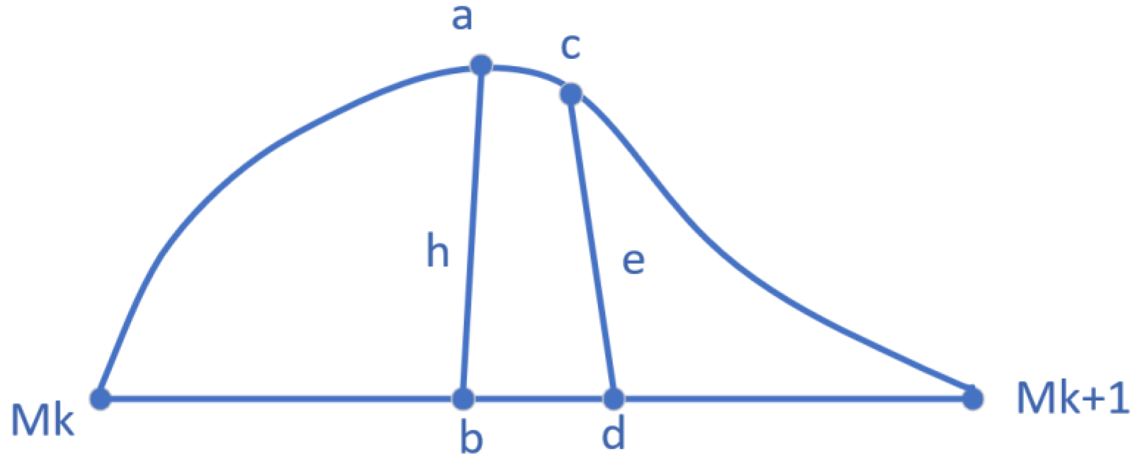
The chord error refers to the maximum normal difference between the chord and arc connecting two endpoints on a curve. To simplify the calculation, the algorithm can be adopted where Mk and Mk+1 are the two interpolation points on the curve, point c is the midpoint of the curve between the two points, and point d is the midpoint of the line between the two points. The two points of cd can be connected, and the modulus of the vector value, |cd|, is referred to as the chord error. The reason for carrying out this process is that the precision of CNC machine tools is generally higher (µm level), and the corresponding strings of the same order of magnitude are generally shorter, so the difference between |cd| and the actual bow height error, |ab|, is very small. Figure 1 shows the midline approximation of the string error.
From the derivation of the interpolation algorithm above, it can be seen that this algorithm is a recursive method with a cumulative error. However, since third-degree B-spline curves are composed of segmented curves, the cumulative error only occurs at each end, which is generally very small and can be ignored. Therefore, the influence of interpolation accuracy is mainly due to the bow height error. From Equation (4), the following formula can be derived:
c d = P u + u 2 [ P u + P ( u + u ) ] 2 = ( 3 R 3 u + 6 R 3 u + 2 R 2 ) × u 2 8
∆u can be ignored to obtain the highest degree:
ε = c d = | 3 R 3 + R 2 | × u 2 4
This equation is the first term of u, so its maximum value is obtained at the boundary of the domain:
ε m a x = u 2 4 m a x 3 R 3 + R 2 , | R 2 |
In order to ensure machining accuracy, the chord error must be lower than the allowable chord error, δ, on the whole third-degree B-spline curve.
u 2 / δ m a x 3 R 3 + R 2 , | R 2 |

3.1.3. Feed Rate Analysis

From Equation (5), using the modulus of the function, we obtain the following:
f = P u = 3 R 3 u 2 + 2 R 2 u + R 1 + 3 R 3 u u + R 3 u 2 + R 2 u u | 3 R 3 u 2 + 2 R 2 + R 1 | u
It can be seen from the above formula that the chord length corresponding to each step is changed due to the incremental calculation of parameters of a fixed step size; that is, the feed rate is not constant. The advantage of this interpolation is that the algorithm is simple and can realize high-speed interpolation.

3.2. Constant Feed Interpolation Algorithm for Cubic Splines

Although the ISO-parametric segmentation interpolation algorithm is simple and fast, it has the following defects:
(1)
The length of each segment chord is not equal, and the tool must pass through them in the same interpolation cycle, so the interpolation speed along the curve is not constant. As a result, the tool vibrates on the machining surface of parts at the end of machining, which unnecessarily prolongs the machining time and reduces the machining quality.
(2)
It is difficult to obtain a reasonable value of ∆u because the optimization value of the parameter ∆u increment is not known in advance. If ∆u is too small, the string step will be too small and the system will slow down; conversely, if ∆u is too large, the string step size will be too large, and the position accuracy will not be satisfied.
(3)
Because it is a recursive method, there is a cumulative error.
The constant-speed real-time interpolation algorithm solves the above problems satisfactorily.

3.2.1. Establishment of Constant-Speed Real-Time Interpolation Algorithm

In order to maintain a constant speed in spline interpolation in the trajectory space, it is necessary to determine the contour step in an interpolation cycle according to the programming feed rate and then map this step into the parameter space to obtain the increment ∆u in the corresponding parameter space. To carry this out, follow these steps:
Let V ¯ be the tangential velocity vector of the spline curve;
V ¯ = d P ( u ) d t = d P ( u ) d u . d u d t
Suppose V is the programming feed rate of the spline curve, then
V = V ¯ = d P u d u . d u d t
d u d t = V | d P u d u |
Applying the differential equation to the equation above,
d 2 u d t 2 = V 2 . d P ( u ) d u . d 2 P ( u ) d u 2 | d P ( u ) d u | 4
Set the interpolation cycle of the control system as T s , t i + 1 t i = T s ; u is a function of time, t .
u t i = u i u t i + 1 = u i + 1
Set, using the Taylor series equation, the expansion of u t i + 1 at t i .
u i + 1 = u 1 + d u d t | t = t i + 1 2 d 2 u d t 2 | t = t i ( t i + 1 t i ) 2 + O t 2
Then, the first-order approximation of the interpolation recursive formula is as follows:
u i + 1 u i + V · T s d P u d u u = u 1
The second-order approximation is as follows:
u i + 1 u i + V · T s d P u d u u = u 1 V 2 · T 2 d P ( u ) d u · d 2 P ( u ) d u 2 2 · | d P ( u ) d u | 4
Since the interpolation cycles, T s , of the present control system are generally very small, the first-order approximate iterative solution can meet the accuracy requirements under the condition that the radius of curvature of the curve is not too small. If the radius of the curvature is small, a second-order approximation is used.
The flowchart of the third-degree B-spline interpolation program with a constant-speed algorithm is shown in Figure 2.

3.2.2. Interpolation Preprocessing

In order to improve the real-time interpolation speed of a spline curve, necessary pre-processing must be carried out before real-time interpolation calculation; that is, correlation coefficients in the interpolation calculation formula must be determined according to input information obtained by the control system.
(1)
Trajectory expression coefficient calculation
When carrying out spline curve interpolation, the input can be both control point information and type value point information. When control point information {P0, P1, P2……Pn} is input, the geometric form of b-spline curve expression is as follows:
P i u = U M P T , i = 0 , 1 , 2 , 3 , n 3
where M is a constant coefficient distance matrix, U = u 3 u 2 u 1 ,   P = P i P i + 1 P i + 2 P i + 3 ; by comparing Equation (4) with Equation (23), we can obtain the following:
R 3 = 1 6 P 1 + 3 P i + 1 3 P i + 2 + P i + 3 R 2 = 1 6 3 P i 6 P i + 1 + 3 P i + 2 R 1 = 1 6 3 P i + 3 P i + 2 R 0 = 1 6 P i + 4 P i + 1 + P i + 2
Equations (A14) and (A15) in Appendix B of the article provide a detailed description of the intermediate steps in the solution of Equation (24). Since n + 1 control points constitute n − 3 spline curves, corresponding coefficients must be dynamically selected according to the curve segment where the interpolation points are located in the interpolation process.
When the input is type value point information {Q0, Q1, Q2……Qn}, the control points of the spline curve must be calculated from these type value points first. Given the n + 1 type value points supplemented with two boundary conditions, the corresponding n + 3 control points {P0, P1, P2……Pn+2} can be obtained using inverse equations. After the control points are determined, the coefficients of the track expressions of various curve segments can be calculated according to Equation (24).
(2)
| d P ( u ) / d u | calculation of coefficients
In spline interpolation, real-time computation is required, d P ( u ) / d u u = u i , to determine the value. In order to reduce the workload of real-time calculation, the coefficient of d P ( u ) / d u can be calculated in advance via interpolation pretreatment.
d P u d u = d x d u 2 + d y d u 2 + d z d u 2 1 2 = a 4 u 4 + a 3 u 3 + a 2 u 2 + a 1 u + a 0 1 2
Among them,
a 4 = 9 R 3 x 2 + R 3 y 2 + R 3 z 2 a 3 = 12 R 3 x R 2 x + R 3 y R 2 y + R 3 z R 2 z a 2 =   4 R 2 x 2 + R 2 y 2 + R 2 z 2 + 6 R 3 x R 1 x + R 3 y R 1 y + R 3 z R 1 z a 1 = 4 R 2 x R 1 x + R 2 y R 1 y + R 2 z R 1 z a 0 = R 1 x 2 + R 1 y 2 + R 1 z 2
(3)
Precision analysis of constant-speed real-time interpolation
The derivation of the constant velocity feed interpolation algorithm shows that the interpolation point is always on the curve without error accumulation, and the feed rate is constant, which affects the interpolation accuracy due to the chord error.
From Equation (24), it can be concluded that there is almost no radial error at u = R 3 / 3 R 2 , the string radial error, ε, is the largest at the boundary u = 0 or u = 1 in the push interpolation algorithm with uniform parameter segmentation, and the radial error distribution fluctuates greatly. However, the extreme distribution of the radial error is 0 u 1 in nonuniform segmentation. If the radius of the curvature of the curve is not too small, the error fluctuation will be small.
(4)
Feed Rate analysis
Because of the parameter increment in each interpolation period,
u 1 = V · T s | d P i u d u | u = u i
Determined via the programming feed rate and interpolation cycle, the chord length of the trajectory space formed during each interpolation cycle is constant; that is, it is the constant speed of the feed.

4. Controller Software and Hardware Design

The aim of our research is to realize the real-time interpolation of a B-spline curve with multi-axis linkage. This will increase the practical application and practicability of the work. Therefore, the practicality and cost performance of the system are mainly considered in the design of hardware and software. If a CNC numerical control system is used, G code is required. However, a B-spline control algorithm is difficult to implement with G code.
According to our evaluation of various embedded systems, using DSP for system design can ensure the high efficiency of algorithm operation, but the implementation cost is high. If a FPGA is used for system design, it will be difficult to realize the design of algorithm logic and the system will suffer from poor scalability. On the premise of ensuring cost performance and design flexibility, this work uses the STM32 series CPU of the ARM system as the core control chip; the specific model is STM32407ZGT6.

4.1. Hardware System Design

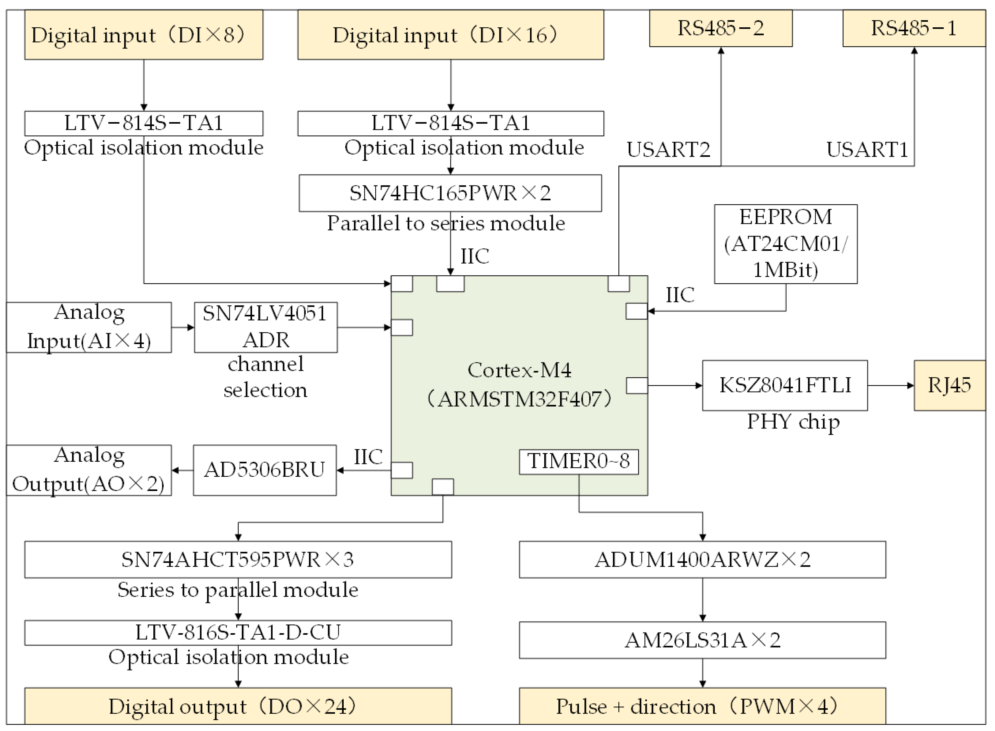
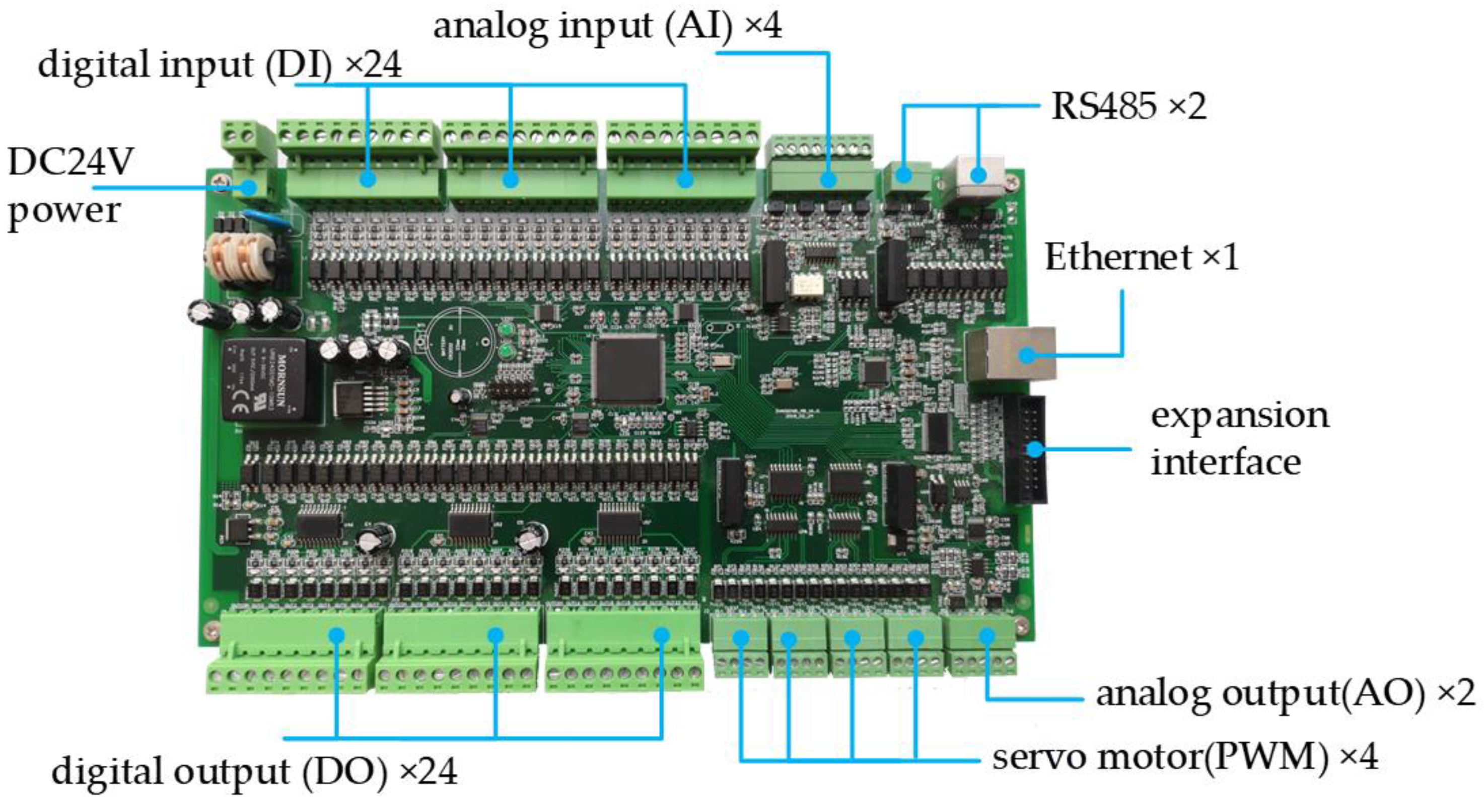
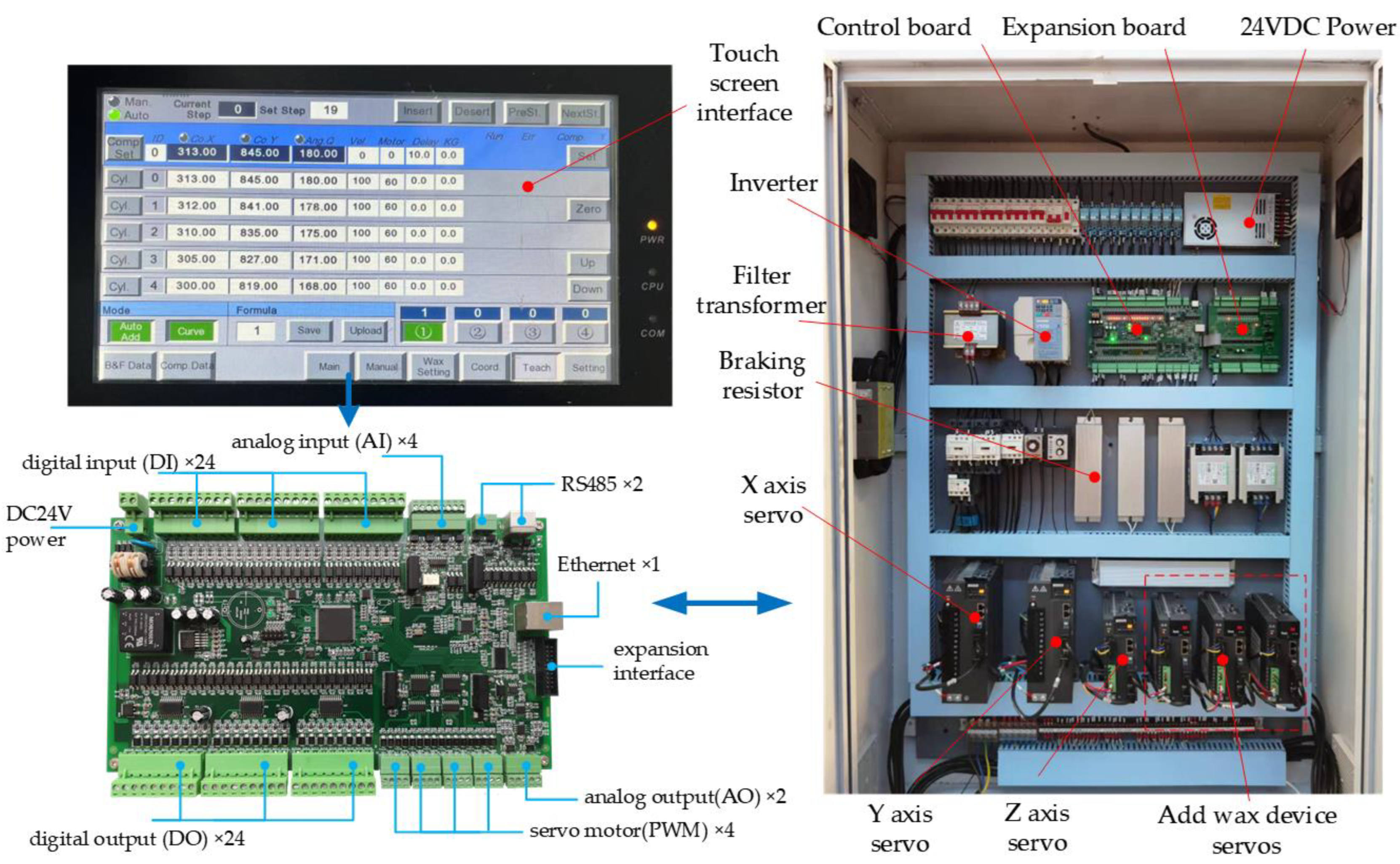
Figure 3 shows the hardware design block diagram of the control system of this work. The controller uses a Cortex-M4 ARM architecture controller, the interface is compact, and the configuration resources of the controller design are as follows: four-channel PWM servo motor control, a two-channel RS485 communication interface, 24-channel digital input, 24-channel digital output, EPPROM(1Mbit), and one Ethernet interface.
Due to the limited hardware interface resources of STM32, in order to make the controller realize the high-speed B-spline interpolation algorithm, the interface resources are optimized in hardware design. The specific design scheme is as follows:
  • The digital input uses an optical coupling isolation chip (LTV-814S-TA1) for input interference isolation. The first eight digital input channels are directly connected to the CPU. For the final 16 digital inputs, due to limited CPU interface resources, a parallel conversion and series chip (SN74HC165PWR) is set for conversion, and the IIC protocol is used for digital reading.
  • The digital output uses an optical coupling isolation chip (LTV-816S-TA1-D-CU) for output anti-interference isolation and, due to the limited interface resources, a parallel-to-serial chip (SN74AHCT595PWR) for output. The CPU uses a serial protocol for 24 digital output control.
  • The analog input uses the analog input interface of the CPU. The channel is selected through the channel selection chip (SN74LV4051ADR) and directly accesses the CPU.
  • In order to save CPU resources, the two analog outputs are sampled using a special analog input chip (AD5306BRU), and the control accuracy is of a 12-bit resolution.
  • The controller design is a two-RS485 interface, using CPU internal USART1 and USART2 realization. Two interfaces are used, one of which realizes human–computer interactive communication with the touch screen. The other is used to realize offline program upgrades and downloads.
  • The controller is designed with a 100 M Ethernet interface and uses a PHY chip (KSZ8041FTLI) to realize Ethernet communication.
  • The multi-axis motor control uses a high-speed CPU timer. The timer output interface runs through the isolation chip (ADUM1400ARWZ) and differential conversion chip (AM26LS31A) output. The control mode is pulse and direction differential control, and the highest output frequency is 200 KHz.
Figure 3 shows the hardware schematic diagram of this work, while Figure 4 shows the hardware circuit board.

4.2. Software System Design

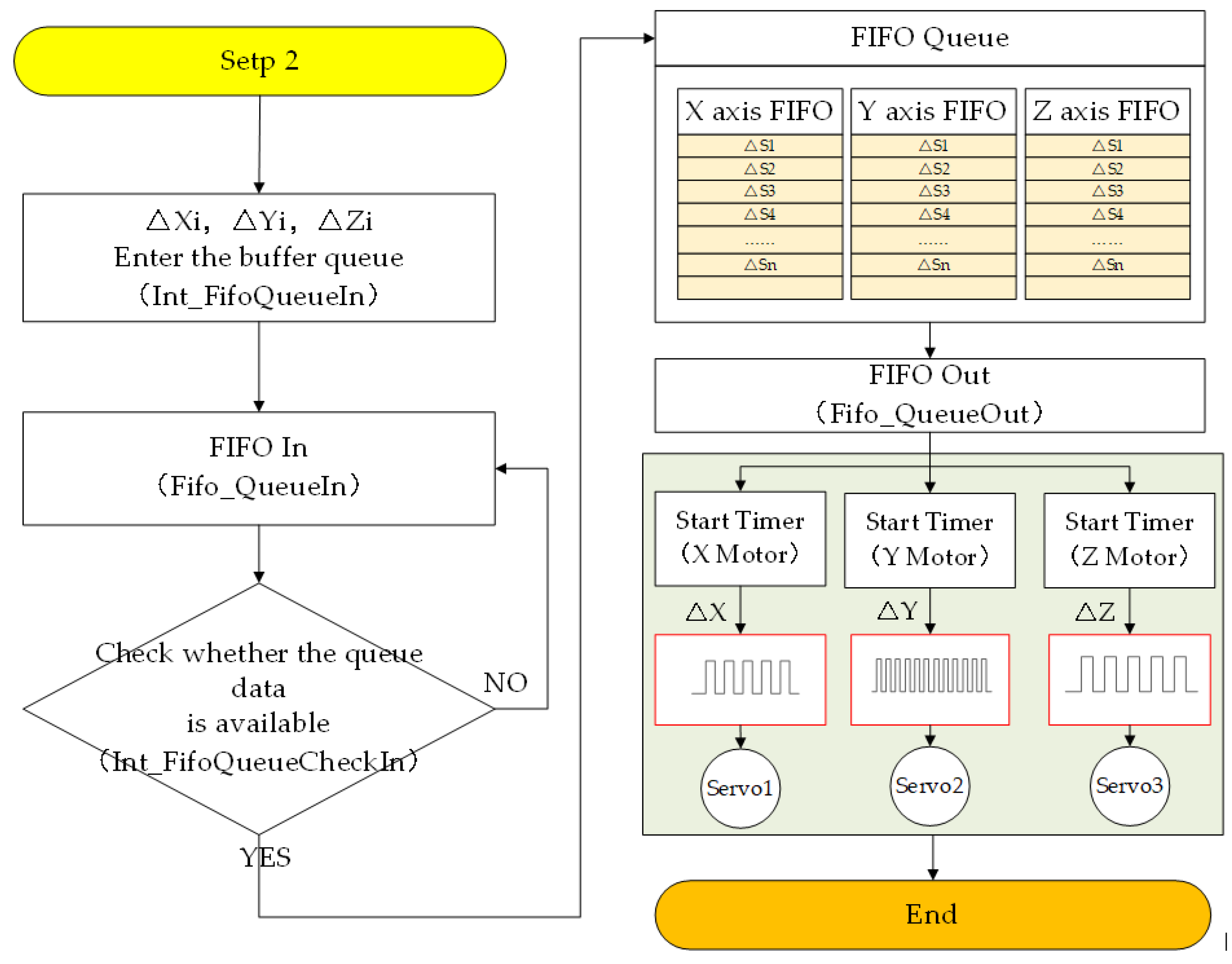
The software system uses C language for program development, and the software framework and implementation process are shown in Figure 5 and Figure 6.
The interpolation cycle, Ts, used in this system is 1 ms. Figure 5 shows the first step of the software interpolation process. After the interpolation process is started, the program will enter the velocity-state flow logic. The acceleration/deceleration strategy can be used to determine which speed state the current trajectory is in. The speed states are idle state, acceleration state (Acc), deceleration state (Dec), and constant-speed state. In the interpolation period, Ts, the real-time interpolation speed, ΔV, can be obtained the via current motion state. After the program calculates ΔVi, it will enter the B-spline function algorithm function (Int_Update_Pos) to calculate the displacement increase in the current interpolation cycle, Ts: ΔXi, ΔYi, and ΔZi.
Figure 6 shows the second step of the software interpolation process. Each axis establishes its own FIFO output buffer, and when there is a spare position in the buffer queue (Int_FifoQueueCheckIn), the displacement increment calculated by the B-spline interpolation algorithm in the last stage will be pushed to the output FIFO buffer of each axis (Int_FifoQueueIn), and the corresponding frequency setting output PWM waveform will drive the servo motor. In order to ensure the real-time response of the interpolation cycle, pulse data conversion and timer control are executed in the CPU interrupt function, which is very efficient. Figure 6 shows the FIFO buffer process diagram.

5. Simulation

The purpose of this study is to verify the real-time application of the three-degree B-spline curve in embedded systems. The theoretical simulation uses MATLAB as an analysis tool, and the simulation data will be verified in the actual three-axis polishing control equipment. The trajectory control points used in this simulation study are obtained after measuring the actual workpiece, and the specific data are shown in Table 1. The interpolated data will be verified on the STM32 embedded system’s control board. The running speed set under the simulation is 100 mm/s. The theoretical simulation curve is shown in Figure 7, which shows the running track, in theory, of the B-spline curve.

6. Experiment

Figure 8 shows the overall framework of the experiment in this work. The experimental equipment is special equipment for CNC polishing that can realize the linkage interpolation movement of the x-, y-, and z- axes (where the z-axis is the rotation axis), and the equipment mainly realizes the polishing of metal utensils.
Figure 9a shows the CNC polishing equipment used in the experiment. The motion axes are indicated in the figure. The CNC polishing equipment is made by Zhaoqing No. 2 Machine Tool Co., Ltd.(Zhaoqing, China), and the controller is the STM32 embedded control system.
Figure 9b is the schematic diagram of the equipment; the figure indicates the running direction of each axis. The x-, y-, and z-axis coordinates of the interpolation process are recorded as P x , P y , and P z , and we used a B-spline curve to plan the three-axis linkage interpolation process. Combined with the analysis provided in Section 3, according to Equations (4) and (23), the corresponding relationship can be obtained as P i = P ( x i , y i , z i ) .
The workpiece is installed on the z-axis of the equipment, controlled by the self-developed embedded control board, so that the outer surface of the workpiece is close to the grinding wheel for polishing and grinding. The experimental process is as follows: the control point of the spline curve is input through the touch screen, and the data are transmitted to the controller through the RS485 port and through the touch screen. The communication protocol is Modbus. The control system obtains the control point ( P i ) of the spline curve, and then uses the B-spline algorithm to calculate the control quantity and drive the servo motor (the software logic described is in Section 3.2). The interpolation cycle used in this experiment is 1 ms.
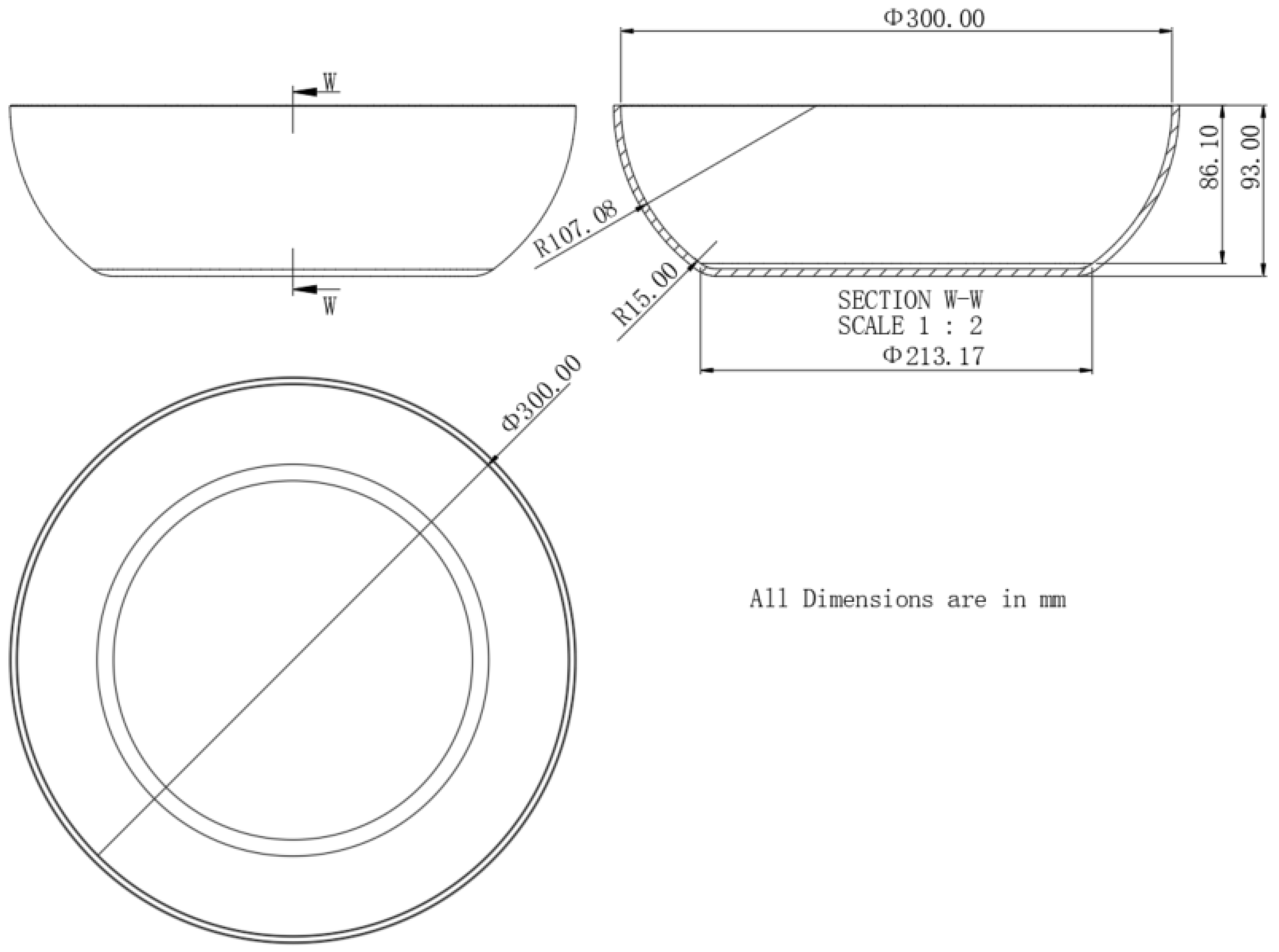
The workpiece used in this experiment is an arc metal utensil cooker. Figure 10 shows the size and shape of the workpiece.
In order to study the B-spline curve motion control algorithm of metal surface polishing, it is necessary to study and analyze the surface polishing process first. In the actual polishing process, the workpiece’s surface is required to contact the grinding wheel surface and carry out relative motion. The smoother the path, the better the polishing effect. Figure 11 is the metal cooker made of stainless steel. The surface of the metal cooker is formed by stamping, and the arc of the surface is a noncircular parabolic arc. In order to use the B-spline curve algorithm to calculate the path trajectory of the curved surface, it is necessary to set the coordinate control points of the curved surface first. Figure 11 shows the locally enlarged surface; P1, P2, P3……Pn−1, and Pn are the obtained discrete control points.
Figure 12 is a schematic diagram of the on-site teaching process of the polishing trajectory, which shows the relative motion of the polishing wheel and workpiece surface and the setting step of the trajectory point. The x- and y-axes are horizontal axis coordinates, the z-axis is the rotation axis, and the value of the z-axis is the swing angle of the workpiece. Images ①–⑨ show the on-site teaching process of the entire polishing trajectory. The data recorded in the process [P1, P2, P3……Pk−1, Pk, Pk+1……Pn−1, Pn] are the actual polishing points, namely the control point of the B-spline algorithm.
Figure 13 shows the actual working process of the CNC polishing equipment in this experiment.

7. Discussion

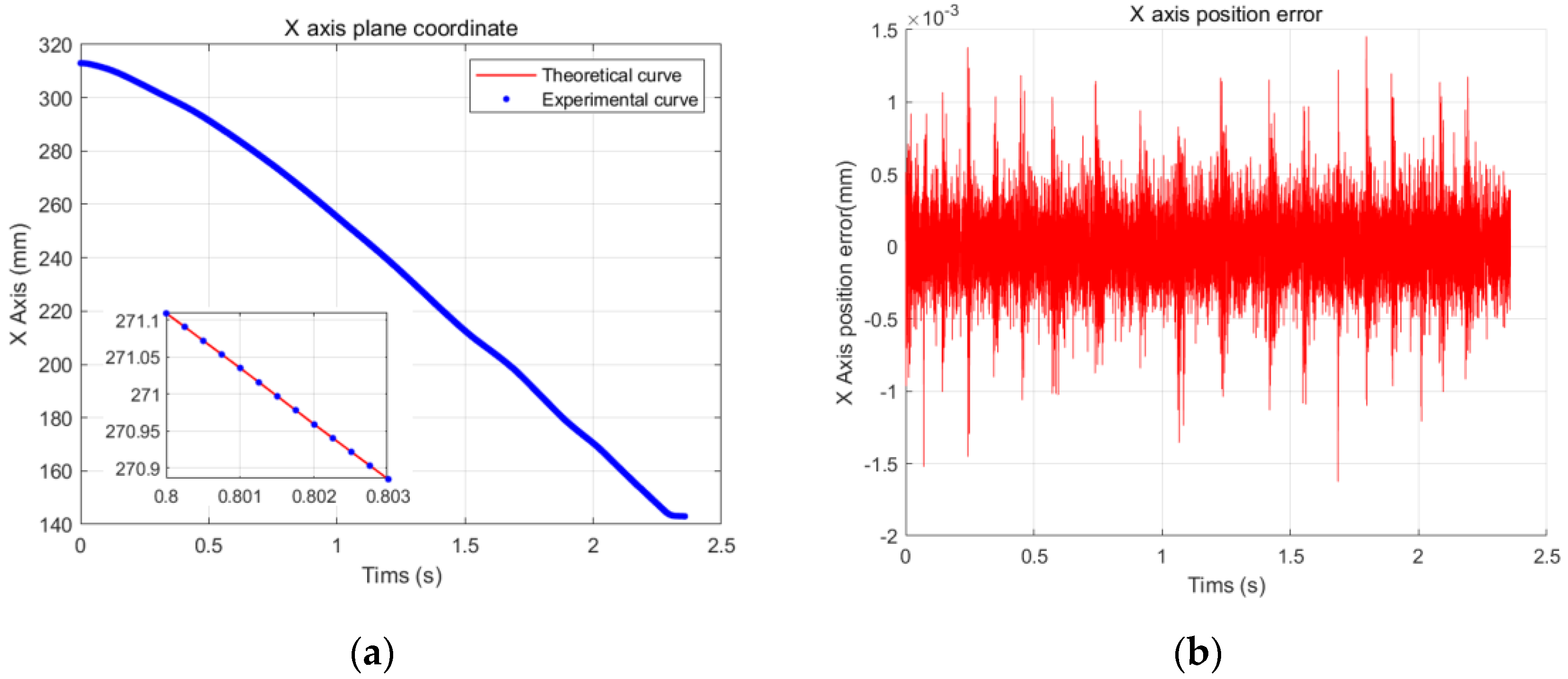
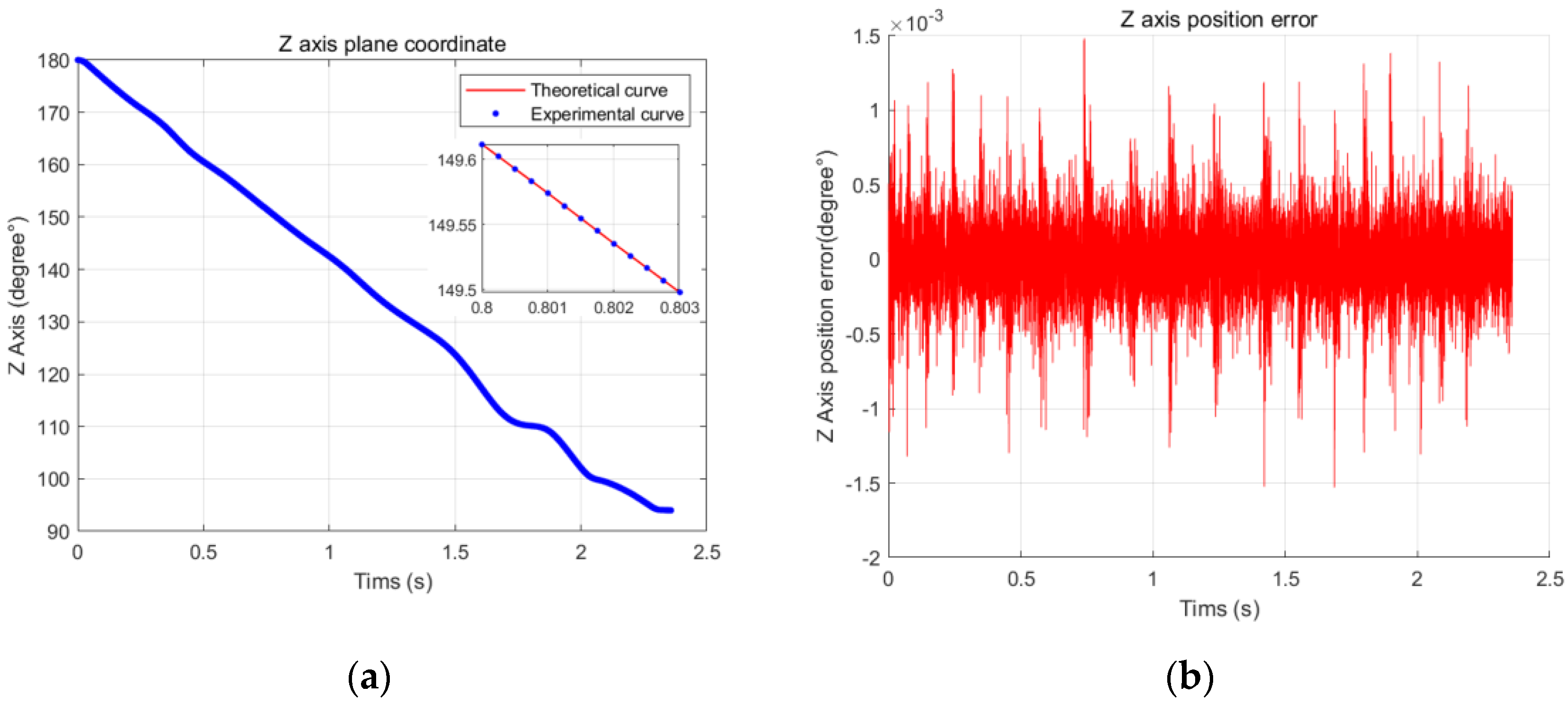
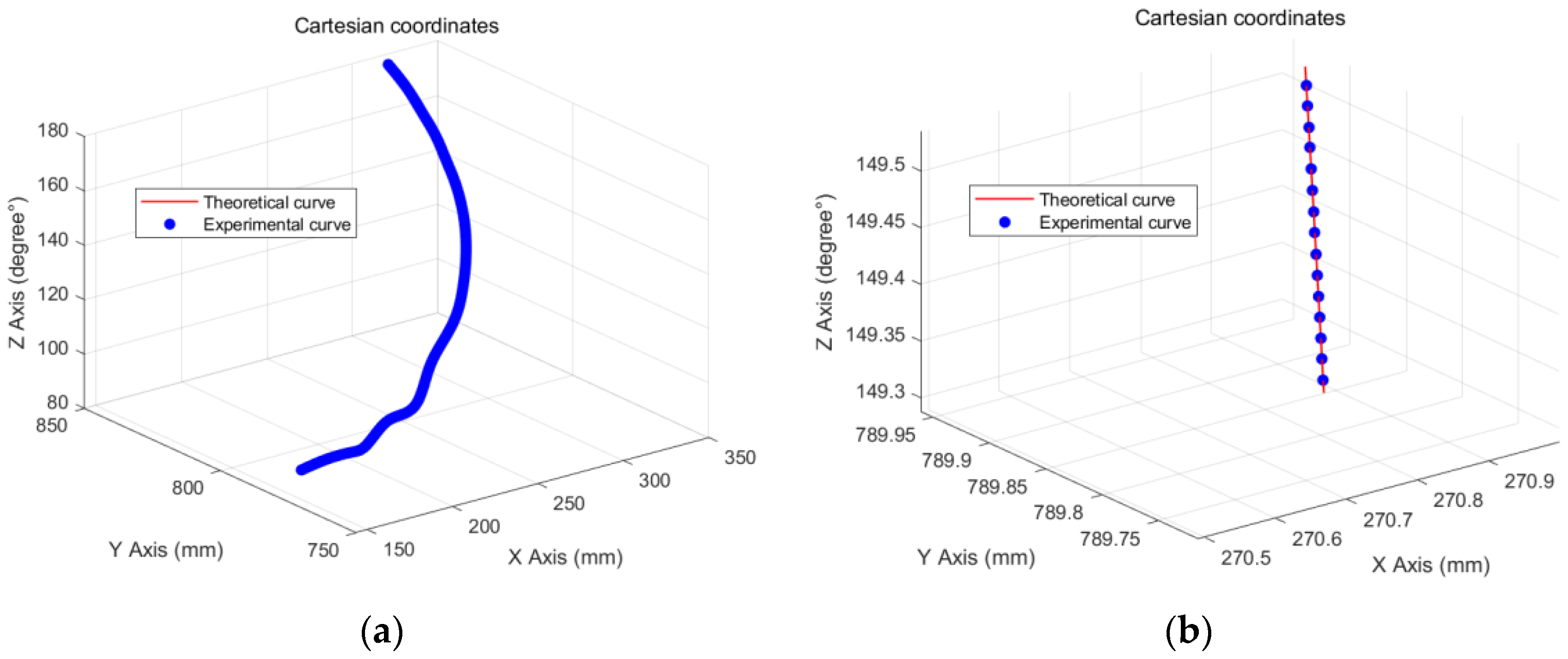
This experiment mainly studies the application of the B-spline curve in real-time interpolation algorithms in embedded systems. According to the polishing process, the running speed is set as 100 mm/s, the acceleration and deceleration are both 2500 mm/s2, the interpolation cycle is 1 ms, and the trajectory error update cycle is 0.125 ms. The system operation effect is shown in Figure 14, Figure 15 and Figure 16. Figure 14a is the actual trajectory curve of the x-axis servo. It can be seen from the trajectory diagram that the x-axis running time is 2.358 s, and the trajectory running range is from 180 mm to 94 mm. Figure 14b shows that the average error value of the trajectory running is 1.098 μm, and the maximum absolute error is 1.796 μm. Figure 15a is the actual track curve of the y-axis servo. It can be seen from the track diagram that the running time of the y-axis is 2.358 s and the track running range is 845 mm~72 mm. Figure 15b shows that the average error value of the track running is 1.284 μm and the maximum absolute error is 1.489 μm. Figure 16a is the actual trajectory curve of the z-axis servo. It can be seen from the trajectory diagram that the z-axis running time is 2.358 s, and the trajectory running range is from 180° to 94°. Figure 16b shows that the maximum absolute error is 0.001685°. Figure 17 shows the running trajectory of the motion axis in a Cartesian coordinate system, and the blue coordinate points are the trajectory of the actual system operation. The experimental data are summarized in Table 2.

8. Conclusions

This paper introduces an embedded control system for the B-spline interpolation of a real-time curve. The system is developed independently, and its main control chip is STM32. It is a low-cost, real-time control scheme. One of the main contributions of this system is the software flow design. The queue function is designed in the software logic to process the interpolated data in real-time and ensure the output of interpolated data within a 1 ms interpolation cycle. The output track is continuously smooth, and the speed and contour are controllable. The hardware circuit design of this project can be compatible with the control of three or more axes at the same time, can realize multi-axis interpolation linkage, and can support an extended analog, Ethernet, and RS485 port.
Another contribution of this work is the design of an embedded control system to implement multi-axis, real-time interpolation. The system uses STM32 architecture for thed esign. This work mainly involves the hardware and software design of an embedded system, especially the discrete optimization of an algorithm to improve the real-time performance of the system. The experimental results show that the trajectory errors of the x-axis, y-axis, and z-axis are all within the expected range, and the errors are very small. The theoretical curve of the B-spline trajectory is basically consistent with the actual curve.

Author Contributions

Conceptualization, Q.T.; methodology, Q.T.; software, Q.T.; validation, Q.T.; formal analysis, Q.T.; investigation, Q.T.; resources, Q.T.; data curation, Q.T.; writing—original draft preparation, Q.T.; writing—review and editing, Q.T.; visualization, Q.T.; supervision, M.A.M.B.; project administration, Q.T. All authors have read and agreed to the published version of the manuscript.

Funding

This research received no external funding.

Data Availability Statement

Data are contained within the article.

Acknowledgments

This project is supported by the Featured Innovation Project of Guangdong Education Department (2021KTSCX141).

Conflicts of Interest

The authors declare no conflict of interest.

Appendix A

The derivation of Equations (8) and (9):
According to Equation (5), we can substitute the variable ( u + u ) into the formula P u to obtain the increasing quantity of P u :
P u = P u + u P u = R 3 u + u 3 + R 2 u + u 3 + R 2 u + u + R 0 P ( u ) = 3 R 3 u u 2 + 3 R 3 u 2 + 2 R 2 u u + ( R 3 u 3 + R 2 u 2 + R 1 u )
Assuming that the constant C 0 = R 3 u 3 + R 2 u 2 + R 1 u , we can obtain the formula for P u :
P u = 3 R 3 u u 2 + 3 R 3 u 2 + 2 R 2 u u + C 0
The calculation of Equation (6) can be extended and associated with Equation (A2):
2 P u = P u + u P u = 3 R 3 u ( u + u ) 2 + 3 R 3 u 2 + 2 R 2 u u + u + C 0 P u = 6 R 3 u 2 u + 6 R 3 u 3 + 2 R 2 u 2
Assuming that the constant C 1 = 6 R 3 u 3 + 2 R 2 u 2 , we can obtain the formula for 2 P u :
2 P u = 6 R 3 u 2 u + C 1
The calculation of Equation (7) can be extended and associated with Equation (A4):
3 P u = 2 P u + u 2 P u = 3 R 3 u 2 u + u + C 1 2 P u = 3 R 3 u 3
This formula no longer contains the variable u ; there will be no new recursion.
From the formula in Equation (5), we can it convert into the following:
P u + u = P u + P u
If we let u i + u = u i + 1 , P i = P u i and u i = u , and combine Equation (A6), we obtain the following formula:
P u + u = P u i + 1 = P i + 1 P i + 1 = P u i = P u P u = P u i = P i
By calculating Equations (A6) and (A7), we obtain the recurrence formula:
P i + 1 = P i + P i
From formula Equation (6), we can convert it into the following:
P u + u = P u + 2 P u
Similarly, if we let u i + u = u i + 1 , P i = P u i , and u i = u , and combine Equation (A8), we obtain the following formula:
P u + u = P u i + 1 = P i + 1 P u i = P i 2 P u = P i
By calculating Equations (A9) and (A10), we obtain the recurrence formula:
P i + 1 = P i + 2 P i
From the formula in Equation (7), we can it convert into the following:
2 P u + u = 2 P u + 3 P u
Using the same steps, we obtain the recurrence formula:
2 P i 1 = 2 P i 2 + 3 P i 2 3 P i 2 = P i
By combining the formulas in Equations (A8), (A11) and (A13), we can derive Equation (8).
By substituting the variable ( i = 0 ) into Equations (4)–(7), we can derive Equation (9).

Appendix B

The derivation of Equation (24):
According to Equation (2), we can convert the equation of a three-degree B-spline curve into the following form:
P i u = j = 0 3 B j , 4 ( u ) P i + j = 1 6 1 u u 2 u 3 1 3 3 1 4 0 6 3 1 3 3 3 0 0 0 1 P i P i + 1 P i + 2 P i + 3
Combined with Equation (23), we can substitute the parameters M, U, and P into the formula and decompose them. The detailed steps are as follows:
P i u = U M P T = 1 6 ( 1 3 u + 3 u 2 u 3 ) 4 6 u 2 + 3 u 3 ( 3 u + 3 u 2 3 u 3 ) u 3 P i P i + 1 P i + 2 P i + 3 = 1 6 [ P i 3 P i + 1 3 P i + 2 + P i + 3 u 3 + 3 P i 6 P i + 1 + 3 P i + 2 u 2 + 3 P i + 3 P i + 2 u + P i + 4 P i + 1 + P i + 2 ] = 1 6 P i 3 P i + 1 3 P i + 2 + P i + 3 u 3 + 1 6 3 P i 6 P i + 1 + 3 P i + 2 u 2 + 1 6 3 P i + 3 P i + 2 u + 1 6 P i + 4 P i + 1 + P i + 2
By comparing Equation (A15) with Equation (4), we can obtain Equation (24).

References

  1. Campos, J.G.; Miguez, L.R. Standard process monitoring and traceability programming in collaborative CAD/CAM/CNC manufacturing scenarios. Comput. Ind. 2011, 623, 311–322. [Google Scholar] [CrossRef]
  2. Shibata, T.; Yano, M.; Kodama, F. Empirical analysis of evolution of product architecture: Fanuc numerical controllers from 1962 to 1997. Res. Policy 2005, 341, 13–31. [Google Scholar] [CrossRef]
  3. Dubovska, R.; Jambor, J.; Majerik, J. Implementation of CAD/CAM System CATIA V5 in Simulation of CNC Machining Process. Procedia Eng. 2014, 69, 638–645. [Google Scholar] [CrossRef]
  4. Pawan Kumar, N.; Mangey, R.; Om Prakash, Y. 7 CNC Machine Programming Codes (G-Codes and M-codes). In Basics of CNC Programming; River Publishers: Aalborg, Denmark, 2018; pp. 73–128. [Google Scholar]
  5. Ji, S.A.; Hu, T.L.; Huang, Z.G.; Zhang, C.R. A NURBS curve interpolator with small feedrate fluctuation based on arc length prediction and correction. Int. J. Adv. Manuf. Technol. 2020, 111, 2095–2104. [Google Scholar] [CrossRef]
  6. Du, X.; Huang, J.; Zhu, L.M.; Ding, H. An error-bounded B-spline curve approximation scheme using dominant points for CNC interpolation of micro-line toolpath. Robot. Comput.-Integr. Manuf. 2020, 64, 101930. [Google Scholar] [CrossRef]
  7. Yang, H.P.; Wang, W.P.; Sun, J.G. Control point adjustment for B-spline curve approximation. Comput.-Aided Des. 2004, 367, 639–652. [Google Scholar] [CrossRef]
  8. Wang, X.D.; Liu, B.; Mei, X.S.; Hou, D.X.; Li, Q.; Sun, Z. Global smoothing for five-axis linear paths based on an adaptive NURBS interpolation algorithm. Int. J. Adv. Manuf. Technol. 2021, 114, 2407–2420. [Google Scholar] [CrossRef]
  9. Zhao, D.; Guo, H. A Trajectory Planning Method for Polishing Optical Elements Based on a Non-Uniform Rational B-Spline Curve. Appl. Sci. 2018, 8, 1355. [Google Scholar] [CrossRef]
  10. Wu, J.; Zhou, H.; Tang, X.; Chen, J. A NURBS interpolation algorithm with continuous feedrate. Int. J. Adv. Manuf. Technol. 2012, 595, 623–632. [Google Scholar] [CrossRef]
  11. Wang, T.Y.; Zhang, Y.B.; Dong, J.C.; Ke, R.J.; Ding, Y.Y. NURBS Interpolator with Adaptive Smooth Feedrate Scheduling and Minimal Feedrate Fluctuation. Int. J. Precis. Eng. Manuf. 2020, 212, 273–290. [Google Scholar] [CrossRef]
  12. Erwinski, K.; Paprocki, M.; Karasek, G. Comparison of NURBS trajectory interpolation algorithms for high-speed motion control systems. In Proceedings of the 2021 IEEE 19th International Power Electronics and Motion Control Conference (PEMC), Gliwice, Poland, 25–29 April 2021; pp. 527–533. [Google Scholar]
  13. Nam, S.H.; Yang, M.Y. A study on a generalized parametric interpolator with real-time jerk-limited acceleration. Comput.-Aided Des. 2004, 361, 27–36. [Google Scholar] [CrossRef]
  14. Ji, S.J.; Lei, L.G.; Zhao, J.; Lu, X.Q.; Gao, H. An adaptive real-time NURBS curve interpolation for 4-axis polishing machine tool. Robot. Comput.-Integr. Manuf. 2021, 67, 102025. [Google Scholar] [CrossRef]
  15. Heng, M.; Erkorkmaz, K. Design of a NURBS interpolator with minimal feed fluctuation and continuous feed modulation capability. Int. J. Mach. Tools Manuf. 2010, 503, 281–293. [Google Scholar] [CrossRef]
  16. Zhang, Y.; Zhao, M.; Ye, P.; Zhang, H. A G4 continuous B-spline transition algorithm for CNC machining with jerk-smooth feedrate scheduling along linear segments. Comput.-Aided Des. 2019, 115, 231–243. [Google Scholar] [CrossRef]
  17. Langeron, J.M.; Duc, E.; Lartigue, C.; Bourdet, P. A new format for 5-axis tool path computation, using Bspline curves. Comput.-Aided Des. 2004, 3612, 1219–1229. [Google Scholar] [CrossRef]
  18. Emami, M.M.; Arezoo, B. A look-ahead command generator with control over trajectory and chord error for NURBS curve with unknown arc length. Comput.-Aided Des. 2010, 427, 625–632. [Google Scholar] [CrossRef]
  19. Liu, X.B.; Ahmad, F.; Yamazaki, K.; Mori, M. Adaptive interpolation scheme for NURBS curves with the integration of machining dynamics. Int. J. Mach. Tools Manuf. 2005, 45, 433–444. [Google Scholar] [CrossRef]
  20. Ni, H.P.; Yuan, J.P.; Ji, S.; Zhang, C.R.; Hu, T.L. Feedrate Scheduling of NURBS Interpolation Based on a Novel Jerk-Continuous ACC/DEC Algorithm. IEEE Access 2018, 6, 66403–66417. [Google Scholar] [CrossRef]
  21. Du, D.S.; Liu, Y.D.; Yan, C.L.; Li, C.X. An accurate adaptive parametric curve interpolator for NURBS curve interpolation. Int. J. Adv. Manuf. Technol. 2007, 32, 999–1008. [Google Scholar] [CrossRef]
  22. Tajima, S.; Sencer, B. Online interpolation of 5-axis machining toolpaths with global blending. Int. J. Mach. Tools Manuf. 2022, 175, 103862. [Google Scholar] [CrossRef]
  23. Xu, B.; Ding, Y.; Ji, W. An interpolation method based on adaptive smooth feedrate scheduling and parameter increment compensation for NURBS curve. ISA Trans. 2022, 128, 633–645. [Google Scholar] [CrossRef]
  24. Du, X.; Wang, B. A C3-continuous NURBS transition scheme for the CNC machining of short linear segments. Precis. Eng. 2022, 73, 1–10. [Google Scholar] [CrossRef]
  25. Yang, Z.; Shen, L.-Y.; Yuan, C.-M.; Gao, X.-S. Curve fitting and optimal interpolation for CNC machining under confined error using quadratic B-splines. Comput.-Aided Des. 2015, 66, 62–72. [Google Scholar] [CrossRef]
  26. Tikhon, M.; Ko, T.J.; Lee, S.H.; Sool Kim, H. NURBS interpolator for constant material removal rate in open NC machine tools. Int. J. Mach. Tools Manuf. 2004, 442, 237–245. [Google Scholar] [CrossRef]
  27. Dharmawardhana, M.; Ratnaweera, A.; Oancea, G. STEP-NC Compliant Intelligent CNC Milling Machine with an Open Architecture Controller. Appl. Sci. 2021, 11, 6223. [Google Scholar] [CrossRef]
  28. Morales-Velazquez, L.; de Jesus Romero-Troncoso, R.; Osornio-Rios, R.A.; Herrera-Ruiz, G.; Cabal-Yepez, E. Open-architecture system based on a reconfigurable hardware–software multi-agent platform for CNC machines. J. Syst. Archit. 2010, 569, 407–418. [Google Scholar] [CrossRef]
  29. Yau, H.-T.; Lin, M.-T.; Tsai, M.-S. Real-time NURBS interpolation using FPGA for high speed motion control. Comput.-Aided Des. 2006, 3810, 1123–1133. [Google Scholar] [CrossRef]
  30. De Santiago-Perez, J.J.; Osornio-Rios, R.A.; Romero-Troncoso, R.J.; Morales-Velazquez, L. FPGA-based hardware CNC interpolator of Bezier, splines, B-splines and NURBS curves for industrial applications. Comput. Ind. Eng. 2013, 664, 925–932. [Google Scholar] [CrossRef]
  31. Jaen-Cuellar, A.Y.; De Santiago-Perez, J.J.; Romero-Troncoso, R.J.; Morales-Velazquez, L.; Benitez-Rangel, J.P.; Osornio-Rios, R.A. A hardware–software system for coordinated multi-axis control based on a non uniform rational B-splines interpolator applied to industrial computer numerically controlled machines. Proc. Inst. Mech. Eng. Part I J. Syst. Control. Eng. 2012, 2266, 831–840. [Google Scholar] [CrossRef]
  32. Fei, J.; Deng, R.; Zhang, Z.; Zhou, M. Research on Embedded CNC Device Based on ARM and FPGA. Procedia Eng. 2011, 16, 818–824. [Google Scholar] [CrossRef]
Figure 1. Midline approximation of the string error.
Machines 11 01043 g001
Figure 2. The flowchart of the spline interpolation program with the constant-speed algorithm.
Machines 11 01043 g002
Figure 3. Flowchart of spline interpolation program with constant-speed algorithm.
Machines 11 01043 g003
Figure 4. Actual hardware circuit board.
Machines 11 01043 g004
Figure 5. Software framework and implementation process (Step 1).
Machines 11 01043 g005
Figure 6. Software framework and implementation process (Step 2).
Machines 11 01043 g006
Figure 7. Simulation (3D B-spline curve).
Machines 11 01043 g007
Figure 8. Overall framework of the experiment.
Machines 11 01043 g008
Figure 9. (a) CNC polishing equipment; (b) schematic diagram of the equipment.
Machines 11 01043 g009
Figure 10. Size and shape of the workpiece.
Machines 11 01043 g010
Figure 11. Diagram of control point of metal workpiece.
Machines 11 01043 g011
Figure 12. Schematic diagram of the on-site teaching process of the polishing trajectory.
Machines 11 01043 g012
Figure 13. Machining process (CNC polishing machine working process).
Machines 11 01043 g013
Figure 14. (a) x-axis trajectory curve; (b) tracking error.
Machines 11 01043 g014
Figure 15. (a) y-axis trajectory curve; (b) tracking error.
Machines 11 01043 g015
Figure 16. (a) z-axis trajectory curve; (b) tracking error.
Machines 11 01043 g016
Figure 17. Three-dimensional curve trajectory: (a) complete motion trajectory; (b) local trajectory amplification.
Machines 11 01043 g017
Table 1. The parameter setting of the B-spline curve.
B-Spline CurveValue
Number of control points20
Axis3
The control points(313 312 310 305 300 295 288 276 262 251 238 218 209 199 188 179 169 164 154 143), (845 841 835 827 819 812 804 793 784 778 772 767 765 762 762 762 763 764 767 770), (180 178 175 171 168 162 159 152 145 141 133 127 122 111 110 110 100 100 98 94)
Table 2. Summary of experimental data 1.
Axis NumberAverage ErrorMaximum ErrorRunning Range
x-axis1.098 μm1.796 μm180 mm~94 mm
y-axis1.284 μm1.489 μm845 mm~72 mm
z-axis0.000876°0.001685°180°~94°
Note: 1 running time, 2.358 s.
Disclaimer/Publisher’s Note: The statements, opinions and data contained in all publications are solely those of the individual author(s) and contributor(s) and not of MDPI and/or the editor(s). MDPI and/or the editor(s) disclaim responsibility for any injury to people or property resulting from any ideas, methods, instructions or products referred to in the content.