A Novel Tribometer and a Comprehensive Testing Method for Rolling-Sliding Conditions

Abstract

This study introduces a method based on fine torque control to evaluate traction in rolling—liding line contacts under small slide-to-roll ratios (SRRs). To accomplish this, we engineered an innovative testing machine—a two-roller tribometer capable of precisely applying resisting torques to one of the rollers. Two types of tests were designed and conducted to validate our method and showcase the capabilities of the novel test setup. The first type, named the “Traction Decay Test”, proved to be effective in evaluating changes in the SRR over time. The second, named the “Torque-Mode Traction Test”, demonstrated its effectiveness in achieving ultra-low SRRs, in the order of 0.01%. As a result, traction curves with high resolution in the low SRR domain were constructed. This advancement provides the means for gaining a deeper understanding of traction coefficients, wear behavior, and tribological performance at ultra-low SRRs across diverse applications.

1. Introduction

Traction in dry and lubricated rolling–sliding contacts has been a subject of study for many decades. Many researchers have focused their attention on studying different tribological phenomena under small slide-to-roll ratios (SRRs), since in numerous engineering applications, rolling contacts operate under these conditions. Widely known examples include dry and lubricated wheel–rail contacts [1,2,3,4,5] and cam–roller follower contacts [6,7,8].

The tractive behavior of a rolling–sliding contact is characterized by its traction curve [9]. Usually, traction curves shown in the literature are based on two-disc machine measurements [1,2,3,4,5,10,11,12]. In these curves, the traction coefficient is plotted against the slide-to-roll ratio (SRR) (or creep ratio, slip ratio, slippage, or creepage), where the latter term(s) quantify the amount of sliding in relation to rolling at the contact. Although the name and calculation of the latter terms used to quantify slippage at the contact differ, in essence, they represent the same thing. For example, the SRR is given by $\frac{u_1-u_2}{u_m}$, where $u_1$ and $u_2$ are the surface velocities of the contacting bodies and $u_m$ is the mean entrainment velocity.

The two-disc machine concept was introduced by Merrit [13] in 1935 to study worm gear performance. The idea behind this development was to drive two contacting discs at different speeds by using a set of gears to generate traction forces at the interface. At present, the integration of advanced speed control systems [14,15] allows the generation of different SRRs in a much more versatile way. Nevertheless, the underlying principle remains the same.

Throughout time, two-disc machines have been used for testing gear contacts [15,16,17,18], cam–roller follower contacts [6,8], and wheel–rail contacts [1,2,4,5,11]. Many publications on wheel–rail contacts are dedicated to the study of traction at SRRs ranging from 0 to 1% ([1,2,3,4,5,11]), where the traction coefficient changes sharply with the SRR. A few publications report traction coefficients at slip ratios below 1%, and as small as 0.1%, with curves containing five or six data points within the range from 0 to 1% slip [1,4,9]. However, many others present curves with fewer data points [2,5,11]. Consequently, the resolution of the traction curves is reduced. In fact, as far as our knowledge extends, there have been no previous reports of traction curves based on two-disc measurements with a larger number (>6) of data points within the SRRs ranging from 0 to 1% and encompassing SRRs below 0.1%.

The situation described above may be attributed to a common issue of twin disc machines that arises at small SRRs. In two-disc tests conducted under speed control, the SRR imposed at the contact is greatly influenced by the sensitivity of the machine, and the traction coefficient is highly sensitive to the SRR, particularly within the range from 0 to 1%. Consequently, even when both discs are driven at “equal speeds,” minimal disparities can lead to traction coefficients above zero being recorded under “pure rolling” conditions [1,5]. Furthermore, while experiments employing two-disc setups and speed control provide valuable insights, they fall short of realistically replicating real-world contact conditions. This inadequacy arises from the fact that rolling contacts in reality do not operate under fixed SRRs, as elaborated below.

To devise an alternative method for assessing traction in rolling–sliding contacts that could yield better results at low SRRs, we have drawn inspiration from the tribological interaction between a cam and a roller follower. In a typical heavily loaded cam–roller follower system (Figure 1), the pin–roller contact functions as a hydrodynamic journal bearing that allows the roller to rotate on its axis by the effect of the traction force $F_t$. At the same time, the friction generated at the pin–roller contact gives rise to a frictional torque ${\tau }_{p-r}$, which can potentially slow down the roller causing slippage at the cam–roller interface. Additionally, at higher speeds, the effects of the inertia torque ${\tau }_I$ generated during accelerations become more significant and can also contribute to the occurrence of slippage at the cam–roller interface. Considering these factors, it can be deduced that the SRR at the cam–roller interface depends on the resisting torque acting on the roller follower. This insight sparked the idea of investigating the sensitivity of an interface in relation to an applied resisting torque, which has proved to be intriguing in previous studies [7].

In this work, we introduce a novel tribometer along with a comprehensive testing method for rolling–sliding line contacts operating under small SRRs. In contrast to the conventional approach based on speed control, our method relies on precise torque control. Since we have drawn inspiration from a cam–roller follower system, we henceforth refer to our novel tribometer as the “Cam-Roller Tribotester (CRT)”. Our method displays a closer resemblance to the operation of many actual rolling contacts and demonstrates effectiveness in generating ultra-small SRRs. As a result, the resolution of traction curves within the small SRR range can be improved. Furthermore, this work describes our novel two-roller tribometer, the CRT (designed to enable precise torque control), and discloses key design aspects. We aim to support future researchers in addressing common issues encountered when using a two-roller (i.e., disc) configuration, including challenges related to contact alignment and the measurement of traction forces.

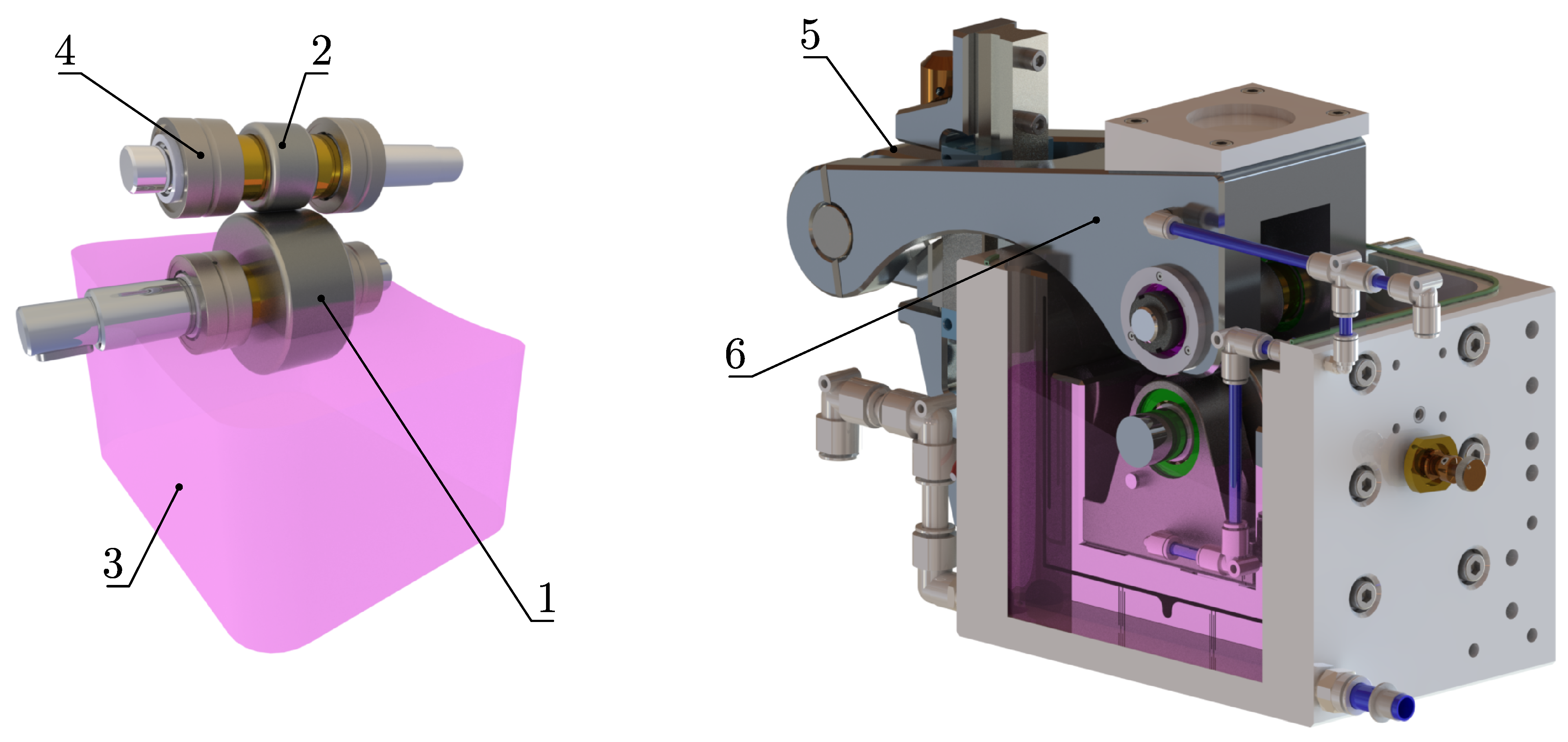
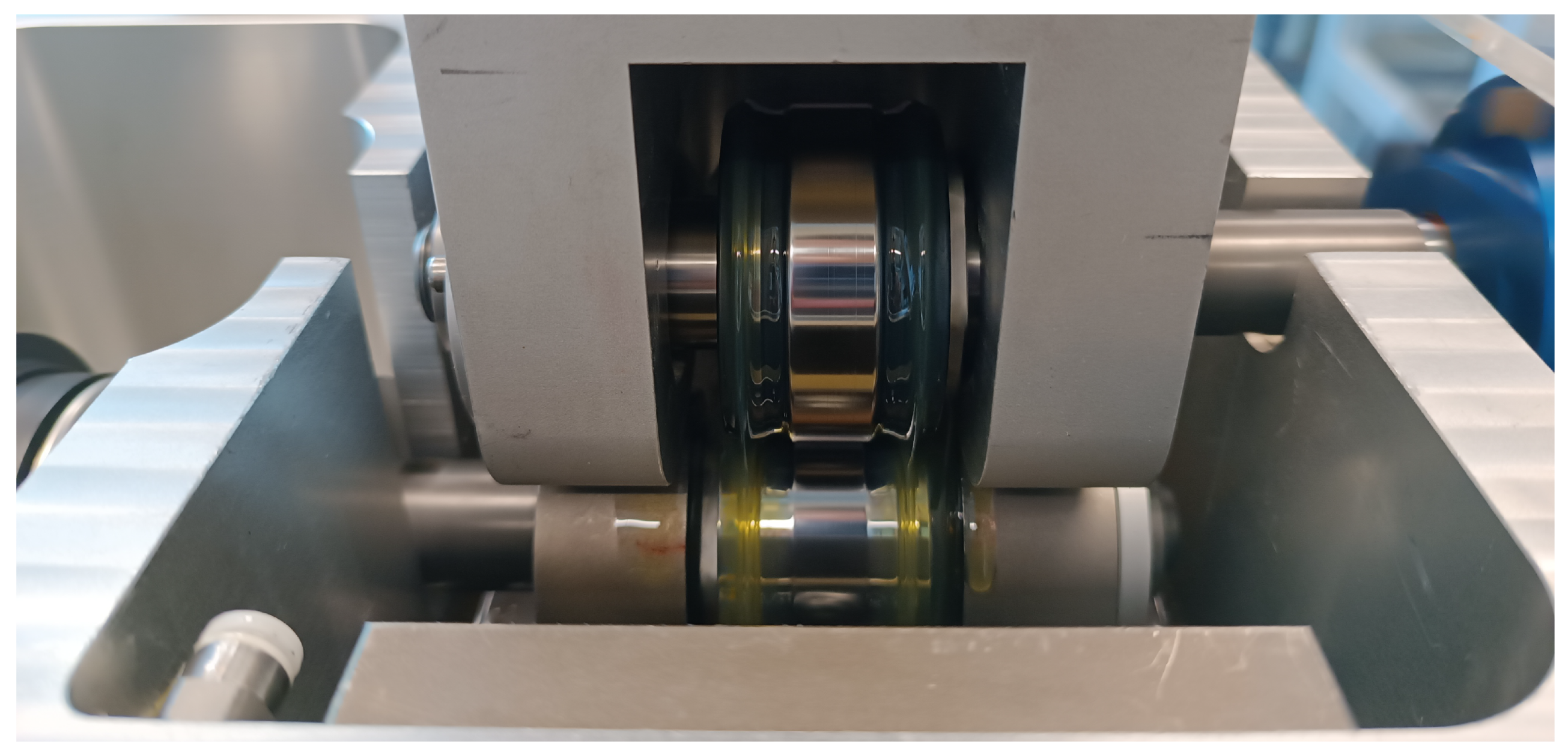
2. The Cam–Roller Tribotester (CRT)

Figure 2 shows a top-level view of the CRT and its systems. The tribological system (1), which takes its name from containing the test rollers in an oil bath, is the core of the test setup and functions as a stiff central support for the other adjacent systems. The driving system (2) is located on the left, the braking system (3) on the right, and the loading system (4) at the top. Figure 3 shows the cross-section of the tribological system. The components forming part of the tribological system include two test rollers, four support bearings, two bearing housings, four heating elements, and other structural components partially submerged in a temperature-controlled oil bath. The lubricant temperature is controlled by employing an autotune temperature controller operating in a closed loop with a K-type thermocouple.

The bottom (1) and top roller (2) are fixed to their shafts, respectively (Figure 3). The needle bearing arrangement (4) allows the shafts to rotate with minimum resistance under high loads while keeping them axially and radially fixed. The lubrication of the needle bearings is carried out by using a two-gear pump with a stable pressure of roughly 7 bar. The lubrication circuit, which comprises external hoses and internal conducts, conveys the oil from an external container to both the top and bottom bearing arrangements. Since the needle bearings do not have seals, the oil can freely flow back into the oil bath and then back to the external container.

2.1. Self-Tracking and Traction Force Measurement

In Figure 3, the pivot point (5) located upstream allows the top roller arm (6) to move with 3 rotational degrees of freedom (DoF) enabling roller self-tracking (similar to a trailer towed by a car), and thus, excellent contact alignment can be attained. To enable self-alignment, the test rollers are mounted on the test setup as shown in Figure 4. First, a moderate load is applied with the air bellow (6), and then, the bottom roller is driven at low speeds (e.g., 50 rpm) for a few seconds. This process takes advantage of the air bellow compliance, the 3 DoF of the top roller arm, and the friction forces at the interface to enable self-alignment of the top roller in the horizontal and vertical planes. By doing so, lateral slippage and localized contact pressures can be prevented during the tests. Once self-alignment has taken place, the top roller shaft is connected to the braking system via flexible couplings (7) (Figure 2). The evenly formed wear track on the bottom roller in Figure 4 confirms that contact along the whole length of the line contact occurred. This serves as evidence that correct alignment has been attained during the test.

To enable the measurement of the traction force $F_t$, the bottom bearing housing is mounted on a flexure-based linear guide, where the DoF coincides with the direction of $F_t$, and hence, frictionless displacement occurs when $F_t>0\mathrm{N}$. By immediately constraining this displacement with a button compression load cell, $F_t$ can be measured with negligible dissipation and without the introduction of parasitic friction forces. Additional details regarding this matter are given in the following sections.

2.2. CRT System Partition

In Figure 2, the driving system (2) employs a high-torque motor (with an inbuilt encoder for speed measurement) connected directly to the bottom roller through a drive shaft to ensure stable speed and torque transfer. The motor is also supported by a flexure-based linear guide to enable frictionless displacement of the whole driveshaft and allow the measurement of traction force. The braking system (3) utilizes a magnetic hysteresis brake (HB-1750) in a closed loop with a high-precision torque sensor (TS109) with an inbuilt encoder and a high-speed controller (DSP7000) to apply precise and stable braking torques on the top roller. In that way, stable traction forces can be generated at the interface. Flexible couplings (7) are used to engage the shafts and compensate for a small misalignment. The loading system (4) generates a contact force $F_c$ using a pressurized air bellow (6). The applied force is measured by a pancake load cell (inline). The force $F_c$ is indirectly controlled by controlling the air bellow pressure via a proportional pressure regulator valve. Finally, the data acquisition system (5) comprises a set of analog and digital I/O NI modules used to operate actuators and acquire data from sensors to store it in a PC. Speed, force, traction, and torque signals are captured by sensors at a 100 $\mathrm{Hz}$ sampling rate, and LabVIEW is used to log data.

Table 1. Technical Specifications of the CRT.

Parameter	Value	Unit
Distance between shafts	54	$\mathrm{m}\mathrm{m}$
Roller length (min./max.)	20/35	$\mathrm{m}\mathrm{m}$
Contact length (min./max.)	4/35	$\mathrm{m}\mathrm{m}$
Contact pressure (min./max.)	0/2.1	$\mathrm{G}\mathrm{Pa}$
Motor speed (max.)	500	rpm
Brake torque (max.)	12	$\mathrm{N}\mathrm{m}$
Load (min./max.)	0/6.7	$\mathrm{k}\mathrm{N}$
Oil temperature (max.)	50	${}^{\circ }\mathrm{C}$
Pancake load cell rated force	8.8	$\mathrm{k}\mathrm{N}$
Compression load cell rated force	2.2	$\mathrm{k}\mathrm{N}$
Torque sensor rated torque	20	$\mathrm{N}\mathrm{m}$
Pancake load cell accuracy	0.1	% of rated load
Compression load cell accuracy	0.25	% of rated load
Torque sensor accuracy	0.05	% of the rated torque
Speed measurement accuracy	0.01	% of the reading
Lubrication type (rollers)	Oil bath	−
Lubrication type (bearings)	Forced lubrication	−

summarizes the specifications of the CRT. Note that rollers with different diameters can be fitted as long as the distance between the axes of the shafts remains 54 $\mathrm{m}$$\mathrm{m}$. To achieve higher or lower contact pressures with the available load range, the contact length can be modified. For example, a maximum contact pressure of $2.1$ $\mathrm{G}$$\mathrm{Pa}$ can be attained with a contact length of 4 $\mathrm{m}$$\mathrm{m}$ and a $6.7$ $\mathrm{k}$$\mathrm{N}$ load (Table 1).

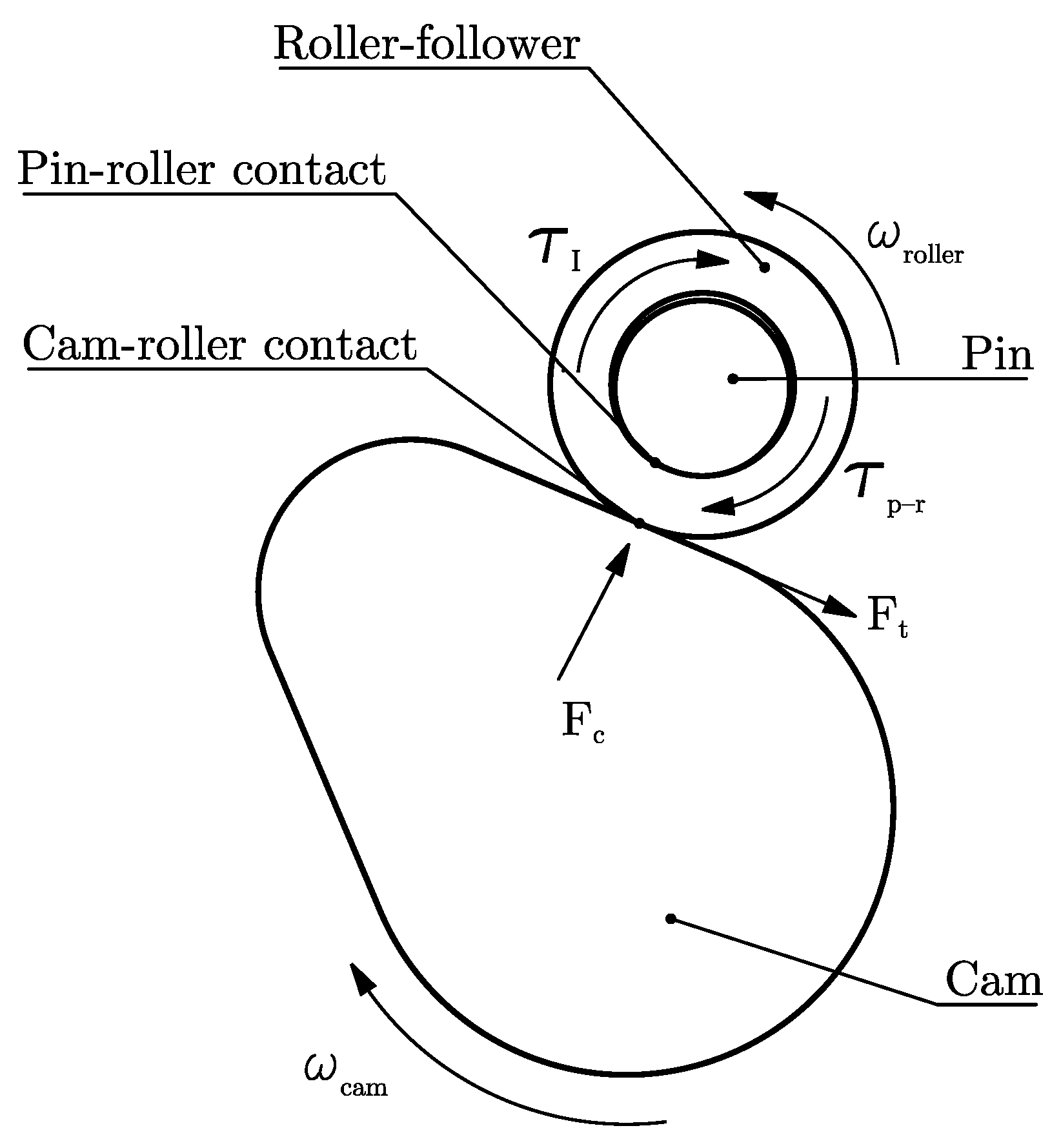
2.3. Force and Torque Measurement Principle

The bottom roller $R_1$ (1) and top roller $R_2$ (2) rotate with angular speeds ${\omega }_1$ and ${\omega }_2$, respectively. The motor drives $R_1$ with a torque ${\tau }_D$, and $R_1$ drives $R_2$. In other words, $R_1$ is driving, and $R_2$ is driven. The contact force $F_c$ generates a maximum contact pressure $P_{\max }$ between the rollers. The small frictional torque ${\tau }_f$ produced by the needle bearings plus the braking torque ${\tau }_B$, act on $R_2$ generating a determined traction force $F_t$ at the interface. In Figure 5, the bearing housing (3) is supported by a flexure-based linear guide (4) that can translate with negligible stiffness in the direction of the traction force $F_t$ and bear high loads in the direction of the contact force $F_c$. A compression button load cell (5) is placed in line with the center of $R_1$ to constrain the linear guide. By doing so, the contact force $F_c$ is kept aligned with the center of the rollers, and the traction force $F_t$ can be measured with negligible dissipation.

2.4. Torque Balancing

Figure 6 shows a simplified top-view schematic of the torques acting on the system. The motor (3) drives $R_1$ with a torque ${\tau }_D$. At the top, $R_2$ is supported by two needle bearings (4a and 4b) that generate a small frictional torque ${\tau }_f$ that acts on $R_2$. The magnetic hysteresis brake (5) is used to apply a braking torque ${\tau }_B$ on $R_2$. Thus, the total resisting torque applied to $R_2$ is the sum of ${\tau }_f$ and ${\tau }_B$, and it is proportional to the traction force $F_t$ acting at the contact. This force is measured by the load cell (7). The torque measured (${\tau }_M$) by the inline torque sensor (6) corresponds only to the braking torque applied by (5). Therefore, ${\tau }_f$ is not accounted for in ${\tau }_M$.

The traction coefficient $\mu =F_t/F_c$ is heavily dependent on the SRR, as dictated by a determined traction curve [9]. The SRR can be computed by balancing torques on $R_2$, as demonstrated in References [7,19,20,21]. Under stable speeds, the torque of inertia (i.e., ${\tau }_I=I{\dot{\omega }}_2$) can be disregarded, and a simplified expression can be written as follows:

$$F_c\mu r_{R2}={\tau }_t={\tau }_f+{\tau }_B$$

(1)

The SRR quantifies the amount of rolling to sliding in the contact and can be calculated with Equation (2), where $u_1$ and $u_2$ are the surface velocities of $R_1$ and $R_2$, respectively, and $u_m$ is the mean entrainment velocity. From Equation (1), it can be deduced that slippage occurs when the “required tractive torque” ${\tau }_f+{\tau }_B$ on the right-hand side of the equation is higher than a limiting available tractive torque at the interface. When this occurs, some slippage must occur until $\mu$ increases up to a point where the torques balance out.

$$SRR=\frac{u_1-u_2}{u_m}$$

(2)

2.5. Frictional Torque

Note that although ${\tau }_f$ is relatively small compared to ${\tau }_B$, it still contributes to the total resisting torque acting on $R_2$ and should be considered. Since the torque sensor can only measure the torques generated by the magnetic hysteresis brake (on the right side), a solution is needed to account for ${\tau }_f$. The tractive torque ${\tau }_t$ can be calculated as $F_c\mu r_{R2}$, where $r_{R2}$ is the radius of $R_2$, and $F_t=F_c\mu$. At stable speeds, the measured torque ${\tau }_M$ is equal to the braking torque ${\tau }_B$ since inertia effects are negligible. By making the respective substitutions in Equation (1), an expression for the total frictional torque ${\tau }_f$ can be obtained (Equation 3). Since $F_c$, $F_t$, and ${\tau }_M$ are continuously measured during the test and $r_{R2}$ is known, ${\tau }_f$ can be calculated as follows:

$${\tau }_f=F_t{r}_{R2}-{\tau }_M$$

(3)

The top and bottom roller shafts use a locating/non-locating bearing arrangement. A combined needle bearing is used for axial and radial support on the locating side, while a single-row needle bearing is used on the non-locating side to accommodate axial displacement due to thermal expansions or component tolerances. The single-row bearing has a mean diameter $d_m$ of 31 $\mathrm{m}$$\mathrm{m}$. The mean bearing diameter of the combined needle bearing $c{d}_m$ is $28.52 \mathrm{m}\mathrm{m}$, respectively ($c=0.92$). The constant c is simply used to express the mean bearing diameter of the combined needle bearing as a function of $d_m$ (i.e., the mean bearing diameter of the single-row needle bearing). Assuming the same friction coefficient (${\mu }_{nb}$) for both bearings and neglecting axial forces and the stiffness of the flexible couplings, Equation (4) can be used to estimate its value. The radial force $F_r$ acting on the bearings can be computed as $F_r=\sqrt{F_c^2+F_t^2}$.

$${\mu }_{nb}=\frac{4{\tau }_f}{F_r{d}_m(1+c)}$$

(4)

It is noteworthy to mention that having the capability to assess the frictional torque produced by the needle bearings opens up interesting possibilities. For instance, the influence of temperature-driven viscosity changes on the frictional torque could be investigated. Although this aspect was not within the scope of the current study, it is certainly one of the opportunities for future research.

3. Testing Method

We designed and conducted two different types of tests, both employing our novel tribometer and the method based on torque control. The first type is referred to as the “Traction Decay Test” and the second as the “Torque-mode Traction Test”.

3.1. Traction Decay Tests

In a traction decay test, a predetermined contact force $F_c$, speed ${\omega }_1$, and braking torque ${\tau }_B$ are set to evaluate the evolution of the SRR during the experiment. This procedure allows for the analysis of the tractive performance of rolling–sliding interfaces over time. Despite the test’s name, it should be noted that the traction force remains constant while the SRR evolves. Thus, an increasing trend in the SRR can be linked to a decline (i.e., decay) in the tractive properties of the interface. In other words, the slipperiness of the interface increases since more slippage is required to balance the same resisting torque (Equation (1)).

Traction decay tests can have various objectives, such as rapidly running-in surfaces, evaluating their endurance, assessing their ability to maintain tractive functional properties over time, studying polishing rates, and identifying the onset of severe adhesive wear, among other purposes. It is important to mention that under controlled torque, better control over the wear rate and wear type might be attained in relation to controlled speed. In traditional two-disc machines, when a scuffing event occurs, the motors will attempt to maintain a stable SRR, resulting in sudden spikes in the tractive torque and severe wear [15]. Conversely, if the SRR is allowed to fluctuate and the traction force is fixed, the occurrence of adhesive wear would lead to a sudden drop in the SRR and negligible changes in the tractive torque.

For the method validation, 3 pairs of 316 stainless steel rollers were employed, where one roller from each pair has a step with a straight length $L_s=10 \mathrm{m}\mathrm{m}$ (Figure 4). The runout was kept below $5 \mathsf{\mu }\mathrm{m}$ by applying low tolerances in the design. During the tests, the rollers were lubricated with a highly refined white mineral oil (Shell Ondina Oil 933) with stable viscosity. The material and lubricant properties are summarized in

Table 2. Material and lubricant properties.

Parameter	Description	Value	Unit
E	Elastic modulus	209	$\mathrm{G}\mathrm{Pa}$
$hd$	Hardness	1.49	$\mathrm{G}\mathrm{Pa}$
$r_{R_1}$	Driving roller ($R_1$) radius	27	$\mathrm{m}\mathrm{m}$
$r_{R_2}$	Driven roller ($R_2$) radius	27	$\mathrm{m}\mathrm{m}$
$L_s$	Straight contact length	10	$\mathrm{m}\mathrm{m}$
$\nu$	Poisson’s ratio	0.33	−
$\alpha$	Pressure–viscosity coefficient	$1.82\times {10}^{-8}$	${\mathrm{Pa}}^{-1}$
${\nu }_k@40 {}^{\circ }\mathrm{C}$	Kinematic viscosity	67	$\mathrm{m}{\mathrm{m}}^2/\mathrm{s}$
${\nu }_k@100 {}^{\circ }\mathrm{C}$	Kinematic viscosity	7.9	$\mathrm{m}{\mathrm{m}}^2/\mathrm{s}$
$\eta @40 {}^{\circ }\mathrm{C}$	Dynamic viscosity	0.058	$\mathrm{Pa}\mathrm{s}$

. For both types of tests, the temperature of the oil bath was maintained at $40 {}^{\circ }\mathrm{C}\pm 2 {}^{\circ }\mathrm{C}$ to stabilize the lubricant viscosity at around $\eta =0.058 \mathrm{Pa}\mathrm{s}$. The lubrication regime was described by using the film parameter $\mathrm{\Lambda }=h_{min}/\sigma$, where $h_{min}$ is the minimum film thickness (estimated with the formulas in Reference [22], and $\sigma =\sqrt{{\sigma }_1^2+{\sigma }_2^2}$, the combined surface roughness. Under some conditions, $\mathrm{\Lambda }$ is smaller than 0.5. In these cases, the lubrication regime is expected to fall in the boundary regime rather than EHL or mixed EHL.

The traction decay tests were conducted first. For that, the 3 pairs of rollers were ground to achieve 3 different roughness levels referred to as smooth (S), medium (M), and rough (R). The initial ${\sigma }_{1i}$ and final ${\sigma }_{1f}$ roughness profiles of the bottom roller were taken for comparison, as well as the initial and final SRRs. All the traction decay tests were conducted in the boundary lubrication regime to ensure contact. For each roughness level, the tests were carried out for $120\min$ under the conditions shown in

Table 3. Reference conditions for traction decay tests.

Parameter	Description	Value	Unit
$F_c$	Contact force	4	$\mathrm{k}\mathrm{N}$
$P_{max}$	Maximum contact pressure	1	$\mathrm{G}\mathrm{Pa}$
n	Driving roller ($R_1$) rotational speed	100	rpm
${\omega }_1$	Driving roller ($R_1$) rotational speed	10.47	$\mathrm{rad}{\mathrm{s}}^{-1}$
${\tau }_B$	Braking torque	7.5	$\mathrm{N}\mathrm{m}$

. During this time, force, torque, and speed signals were acquired at a sampling rate of $100\mathrm{Hz}$.

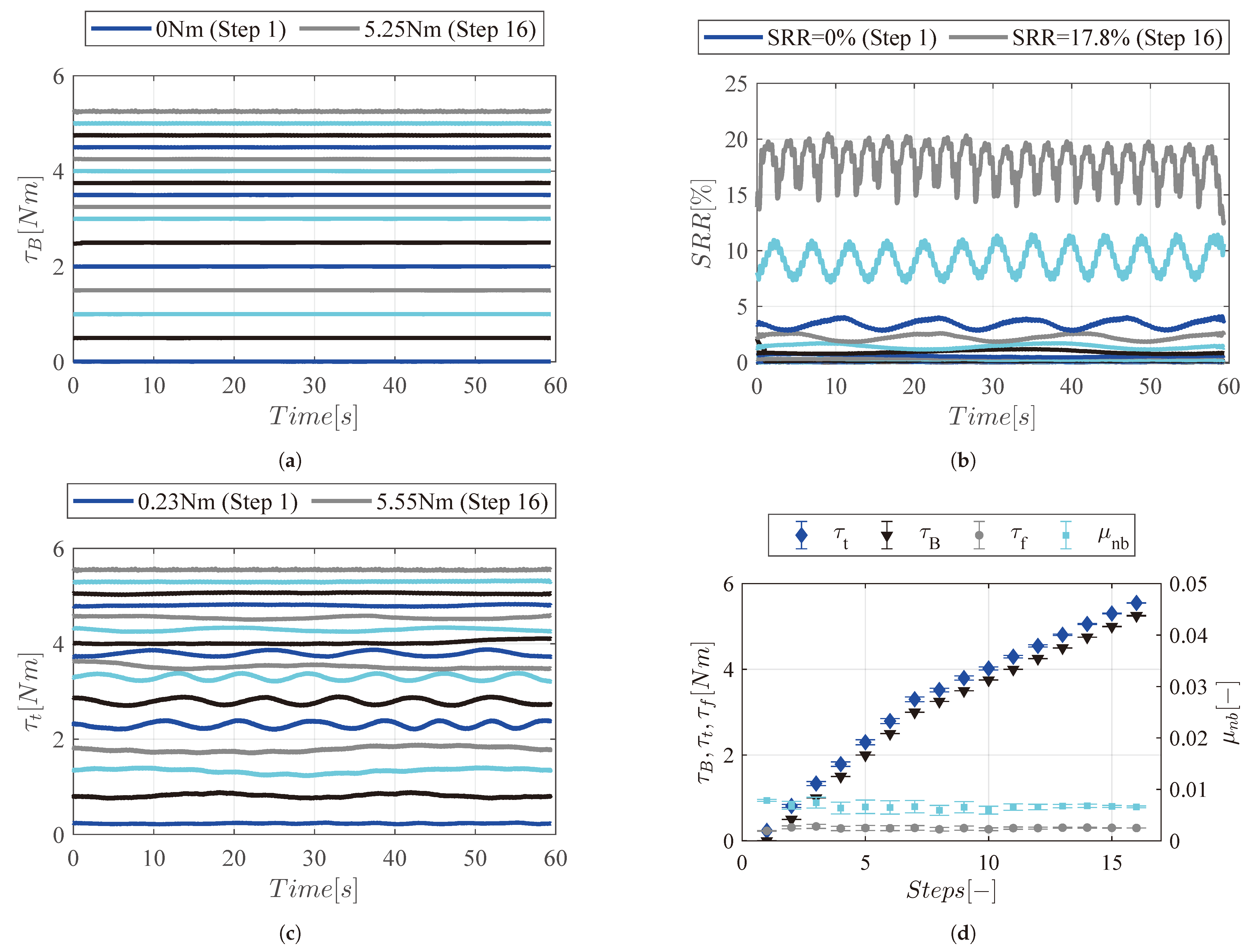
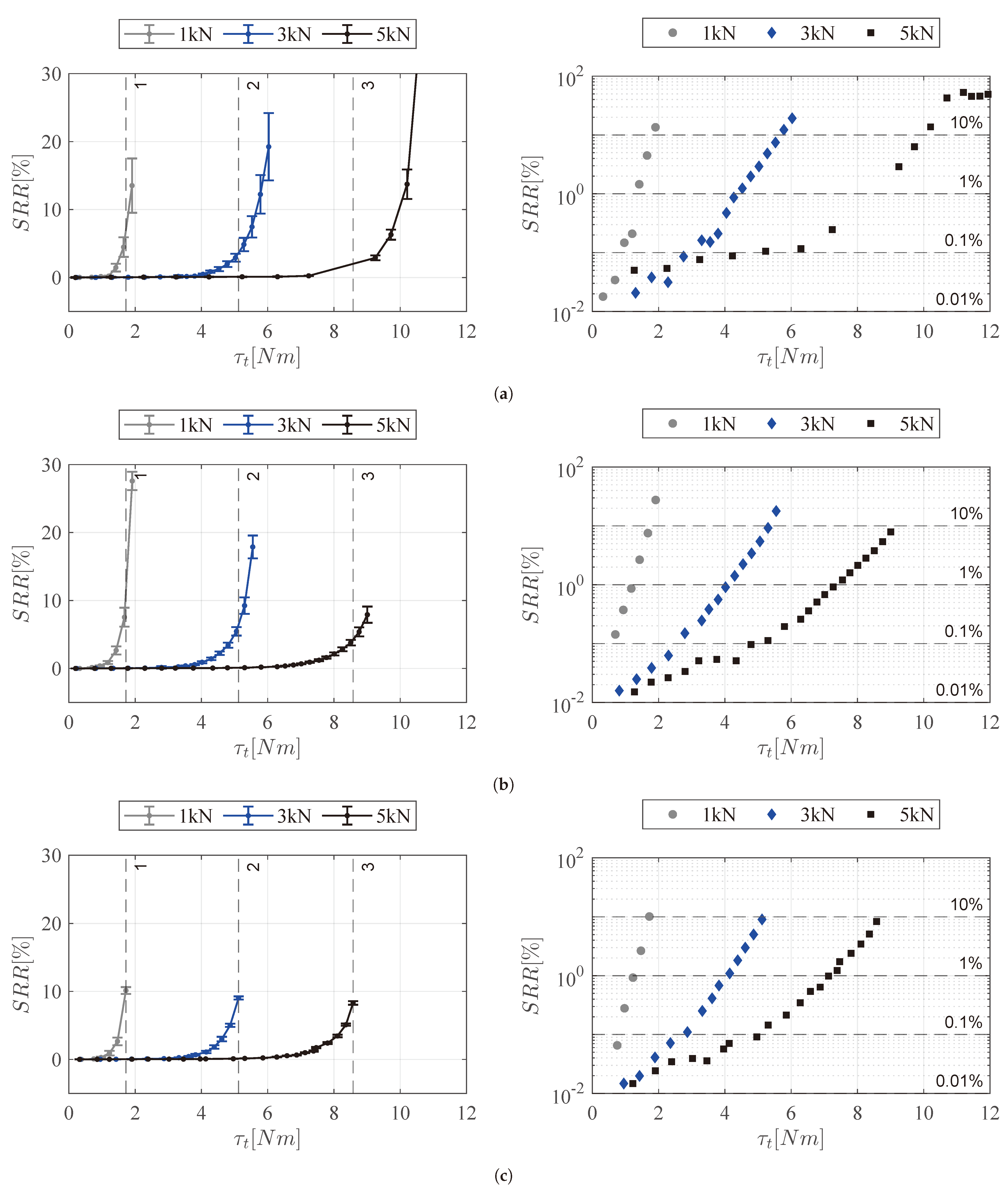
3.2. Torque-Mode Traction Tests

To generate a traction curve in torque mode, the contact force $F_c$ and the speed of the bottom roller ${\omega }_1$ are maintained at a fixed level, the braking torque ${\tau }_B$ is gradually increased in small steps (from low to high), and the resulting SRR is recorded. To construct the curves, the average traction coefficients can be plotted against the SRRs in a conventional traction curve plot [9], or in torque mode as shown in the results. Torque-mode traction curves are useful to investigate the sensitivity of rolling–sliding interfaces as a function of an applied torque. Under torque control, the onset of high SRRs and the maximum transferable traction force of rolling interfaces can be evaluated. For instance, considering a cam–roller system, the impact of pin–roller friction on the tribological performance of the cam–roller contact can be simulated through the application of a resisting torque that mimics the frictional torque at the pin–roller contact. Precise torque control provides the opportunity to mimic different frictional torques produced by the latter contact.

Generally speaking, torque-mode traction tests can be advantageous in evaluating friction-based transmissions and contacts operating under tractive rolling or rolling–sliding conditions. Common examples include backup rolls, support rolls, and wheel–rail contacts since torque control is much closer to the actual tribological system. Furthermore, the ability to finely control the resisting torque is advantageous for producing ultra-low SRRs. This methodology is particularly useful within the linear region of the traction curve, where the traction coefficient varies greatly with the SRR.

To conduct the torque-mode traction tests, the rolling pair with medium surface roughness was re-used, once the traction decay tests (described previously) were concluded. To validate the method over a wide range of conditions, 9 traction curves were generated at 3 different loads and 3 different speeds. The reference conditions for each test are summarized in

Table 4. Reference conditions for torque-mode traction tests.

Speed/Load	1 kN (0.52 GPa)	3 kN (0.91 GPa)	5k N (1.17 GPa)
450 rpm	(1) $\mathrm{\Lambda }=1.43$	(2) $\mathrm{\Lambda }=1.25$	(3) $\mathrm{\Lambda }=1.18$
150 rpm	(4) $\mathrm{\Lambda }=0.81$	(5) $\mathrm{\Lambda }=0.67$	(6) $\mathrm{\Lambda }=0.62$
50 rpm	(7) $\mathrm{\Lambda }=0.54$	(8) $\mathrm{\Lambda }=0.42$	(9) $\mathrm{\Lambda }=0.37$

. These tests were conducted in a determined sequence, from “least critical” (1) to “most critical” (9) conditions, to prevent excessive surface damage. The data were acquired in the same way as explained in the traction decay test above.

3.3. Roughness Measurements

The standard deviation of surface heights ${\sigma }_1$ and ${\sigma }_2$ was measured using a 3D profiler Sensofar S Neox optical microscope in confocal mode with 10× magnification. The measurements were taken before and after the tests. Each surface was marked to ensure matching with the first measurement location, allowing for a clear comparison of roughness changes. The surface profiles were taken perpendicular to the rolling direction. For rollers without a step, the entire contact length was measured along with approximately $2\mathrm{m}\mathrm{m}$ on either side outside of the contact. Roughness values were obtained from a series of profiles taken within the contact after removing initial curvature using low- and high-pass Gaussian filters of $0.8 \mathsf{\mu }\mathrm{m}$ and $2.5 \mathsf{\mu }\mathrm{m}$, respectively, following the ISO 21920 standard [23].

4. Results and Discussion

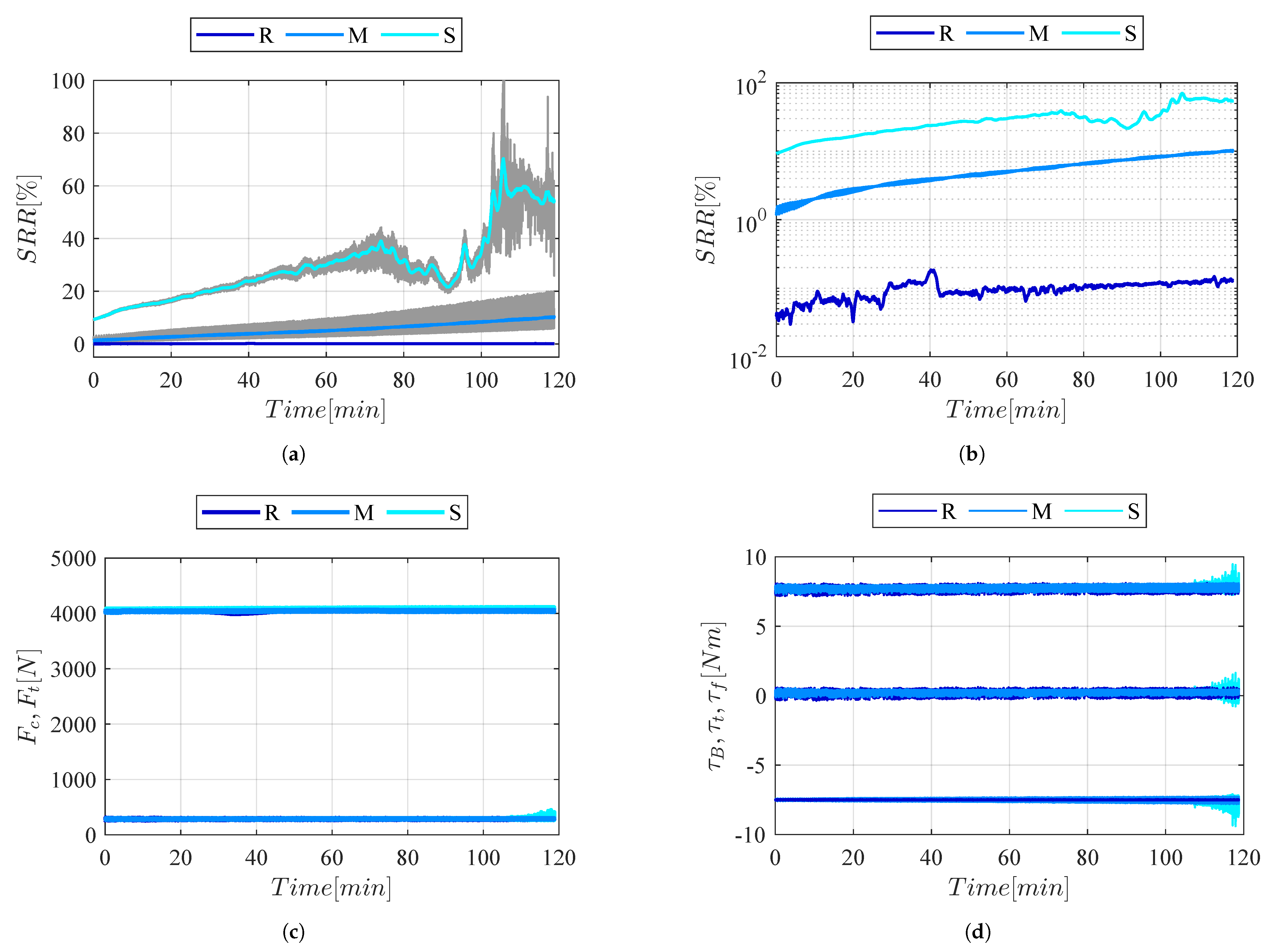
4.1. Traction Decay Tests

Figure 7 shows the data from the traction decay tests for three rolling pairs with three different roughness levels: smooth (S), medium (M), and rough (R), respectively. Figure 7a shows the evolution of the SRR during the tests. The grey background lines correspond to the raw data, and the colored lines on top were obtained by applying a moving average filter. A comparison between the initial and final roughness levels and SRRs is given in

Table 5. Roughness and SRR changes.

Surface Finish	${\mathit{\sigma }}_{1\mathit{i}}$ ($\mathsf{\mu }$m)	${\mathit{\sigma }}_{1\mathit{f}}$ ($\mathsf{\mu }$m)	$\frac{{\mathit{\sigma }}_{1\mathit{i}}}{{\mathit{\sigma }}_{1\mathit{f}}}$	$\mathbf{\Lambda }$	${\mathit{SRR}}_{\mathit{i}}$ (%)	${\mathit{SRR}}_{\mathit{f}}$ (%)	${\mathit{SRR}}_{\mathit{f}}$/${\mathit{SRR}}_{\mathit{i}}$
Smooth	0.32	1.44	0.22	0.44	8.14	54.6	6.7
Medium	1	0.24	4.16	0.28	0.57	10.2	17.9
Rough	2.7	1.3	2.07	0.25	0.019	0.13	6.8

. Figure 7b shows the evolution of the SRR in the logarithmic scale. This plot exposes the ultra-low initial SRR measured with the rough rollers and its increase with time. Figure 7c shows the contact force $F_c$ and traction force $F_t$, which were maintained at a stable level for all roughness levels. Finally, Figure 7d shows the applied braking torque ${\tau }_B$, the tractive torque ${\tau }_t$, and the frictional torque ${\tau }_f$. Note that the braking torque ${\tau }_B$ is shown as negative only for the sake of clarity since its value is very close to that of the tractive torque ${\tau }_t$. This means that the contribution of the needle bearings to the total resisting torque is minimal (Equation (1)). In fact, the average frictional torque is $0.20 \mathrm{N}\mathrm{m}$ and accounts for only ≈2.6% of the total resisting torque. The average frictional torque ${\tau }_f$ generated by the needle bearings corresponds to an average friction coefficient ${\mu }_{nb}=0.0033$.

During the traction decay tests, for all roughness levels (i.e., S, M, and R), a substantial increase in slipperiness was recorded. The rough and smooth surfaces exhibited the smallest and largest SRRs, respectively. However, in Table 5, it is interesting to see that, proportionally, the increase in the SRR was practically the same for both roughness levels. The most significant rise in the SRR occurred with the medium roughness level, where the SRR increased 17.9 times during the test. This considerable increase in slipperiness can be attributed to the loss of roughness caused by polishing wear. The change in roughness for the medium roughness level was the largest compared to the other two (Table 5). Here, it should be noted that the initial SRR (i.e., 0.57%) in Table 5 does not match that in Figure 7b. The reason for this is that 0.57% corresponds to the initial SRR recorded before applying a moving average filter. The same explanation applies to the smooth and rough rollers.

For the rough rollers, a (smaller) decrease in roughness was also observed. However, for the smooth surface, the roughness “increased” during the test. This was attributed to the occurrence of severe adhesive wear, which also explains the large fluctuations in the SRR in Figure 7a. The sudden decline in the SRR in minute 75 and the subsequent fluctuations were linked to the occurrence of severe adhesive wear. Figure 8, Figure 9 and Figure 10 show the initial and final surface topologies of the rollers with rough, smooth, and medium roughness levels.

It should be pointed out that while we recognize the importance of achieving repeatable results, our primary goal in this study was to present our methodology and validate our novel tribometer. Consequently, we stopped ourselves from diving into the details of adhesive wear initiation and the repeatability of such outcomes since conducting such an investigation would demand a substantial number of rolling pairs and a different research design. However, based on the patterns observed and the insights gathered during testing, we believe that comparable outcomes may be anticipated when repeating the experiment with a smooth surface. This anticipation holds valid particularly for smooth stainless steel rollers, given the susceptibility of the material to suffer from adhesive wear.

4.2. Torque-Mode Traction Tests

Figure 11 shows the data acquired to construct one traction curve. In this case, curve (5) according to the sequence in Table 4. It should be noted that in Figure 11, only two legends are shown due to limited space. They correspond to the first and last steps followed, from low to high braking torques ${\tau }_B$, to generate different SRRs. The color of the lines can be used as a guide to distinguish torques and SRRs from different steps.

In this section, the procedure to construct a traction curve is further described, with aid from the results obtained. Figure 11a shows the steps taken in the braking torque ${\tau }_B$ from low to high. At each step, the braking torque ${\tau }_B$ was kept stable for 60 $\mathrm{s}$, while speed, force, and torque signals were acquired. Figure 11b shows the SRRs recorded during the test for each applied braking torque ${\tau }_B$. Low SRRs correspond to small braking torques and vice versa. For example, for the largest average braking torque ${\tau }_t=5.25\mathrm{Nm}$, the mean SRR is 17.8%. It is worthwhile pointing out that fluctuations in the SRR were recorded at larger braking torques in particular. The amplitude of these fluctuations increases proportionally with the braking torque ${\tau }_B$. At low SRRs, the fluctuations are too small to be noticed. This intriguing behavior can be better explained by examining curve (5) in Figure 12b (at $3 \mathrm{k}\mathrm{N}$. At small resisting torques, ${\tau }_t$ values, the slope of the curve is close to zero. Therefore, small fluctuations in the resisting torque ${\tau }_t$ cause much smaller fluctuations in the SRR. However, at higher resisting torques ${\tau }_t$, the slope becomes much steeper. Under these conditions, small fluctuations in the resisting torque cause noticeable variations in the SRR. At ${\tau }_t=5.55\mathrm{Nm}$, the slope of the curve is close to 1. This means that small torque fluctuations cause very large changes in the SRR. Under these conditions, the contact is highly unstable, and full sliding (i.e., SRR = 200%) can suddenly occur. This argument also explains why torque control is attractive, particularly for conducting tests at small SRRs, close to the linear region of the traction curve.

The increasing amplitude of the SRR fluctuations at higher resisting torques is an attention-grabbing aspect. An escalating amplitude could be used to indicate that the limiting traction that the interface can handle is about to be reached. Furthermore, the frequency of the SRR fluctuations (Figure 11b) also appears to increase at higher torques, where more slippage occurs. This phenomenon might be linked to viscosity changes due to thermal effects as follows: At low SRRs, the contact cools down, viscosity increases, and asperity contact is lost; thus, the SRR goes up. At higher SRRs, the contact temperature increases, and viscosity drops, allowing for more contact between asperities, and hence, the SRR goes down. This behavior seems to follow a repeating and predictable pattern, making it an intriguing topic for further investigation.

In addition, the following should be highlighted. Although the braking torque was increased in steps as small as $0.25 \mathrm{Nm}$ for constructing the traction curves, much smaller increments can be made if required. As a result, the number of average data points can be increased, yielding traction curves with improved resolution. In fact, the CRT allows us to apply braking torques with increments as small as $0.1 \mathrm{Nm}$. Concerning the stability of the braking torque, under closed-loop regulation, variations of roughly ±0.05% of the set torque value can be anticipated.

Figure 12 shows nine torque-mode traction curves for three different contact forces ($1 \mathrm{k}\mathrm{N}$, $3 \mathrm{k}\mathrm{N}$, $5 \mathrm{k}\mathrm{N}$) and three different rotational speeds (50, 150, and 450 rpm). On the right side, the logarithmic plots depict the ultra-low SRRs generated at small resisting torques. Using curve Figure 12b (at $5 \mathrm{k}\mathrm{N}$ and $150 \mathrm{rpm}$) as an example, it can be seen that it contains data points at ultra-low SRRs ranging from 0.015% to 0.11% and a total of 15 data points from 0 to 1%. This demonstrates the advantage of operating in torque mode when generating high-resolution traction curves that include ultra-small SRRs.

Overall, it can be concluded that the SRR increases as a function of the resisting torque ${\tau }_t$, except in cases where traction is “enhanced” due to adhesive wear damage. At higher contact forces, the interface can tolerate higher resisting torques at small SRRs. At higher speeds, the tractive properties of the interface decrease due to a reduction in the contact between asperities produced by a thicker lubricating film. For the plots on the left side, the vertical lines 1, 2, and 3 can be used to highlight the influence of speed. For example, in Figure 12c, line 2 intersects the $3 \mathrm{k}\mathrm{N}$ curve at an SRR of 9%, in Figure 12b, at 6%, and in Figure 12a, at 3%. This indicates that at higher speeds, more slippage is necessary to balance the same resisting torques.

It is worth emphasizing that the limited kinetic power rating of a magnetic hysteresis brake can become a constraint. This rating is determined by both the operating speed and braking torque. For the HB1750 model, under continuous operation it should not exceed 350 $\mathrm{W}$. However, for a brief 5 $\min$ period, the maximum allowable kinetic power is 1200 $\mathrm{W}$. During the tests conducted at 450 rpm, in the last four steps with braking torques above $7.5$ Nm, the kinetic power exceeded 350 $\mathrm{W}$. In the final and most critical step, the kinetic power reached 400 $\mathrm{W}$. Notably, these last steps resulted in a significant temperature increase in the brake. Under these circumstances, a fan or compressed air can be used on the side of the brake to improve the dissipation. However, it is essential to be cautious to prevent overheating. In addition, these constraints should be considered when establishing the parameters for testing.

To conclude this section, it is important to point out that the data from the curves in Figure 12 can also be plotted in a conventional way, with the SRR in the x-axis and the traction coefficient $\mu$ (or the tractive torque ${\tau }_t$) in the y-axis. In fact, if the curves in Figure 12 are mirrored on the right and then rotated $90{}^{\circ }$ clockwise, the plots become conventional traction curves, as shown in Figure 13.

5. Conclusions

A novel tribometer, along with a comprehensive testing method for rolling–sliding line contacts operating under small SRRs, was introduced in this work.

In contrast to conventional methods based on speed control, the presented approach relies on precise torque control. This results in a closer resemblance to the operation of many rolling contacts in engineering applications (e.g., cam–roller follower contacts), where slippage occurs as a result of a resisting torque acting on one of the rolling elements.

To validate our method, two types of tests were conducted, namely, the “Traction Decay Tests” and the “Torque Mode Traction Tests”. During the latter tests, our method proved to be effective in generating ultra-small slide-to-roll ratios. As a result, traction curves containing several data points in the range from SRR = 0% to SRR = 1% and encompassing ultra-low SRRs as small as 0.015% were constructed. During the traction decay tests, it was demonstrated that torque control allows us to track changes in the SRR as a function of time. Under stable testing conditions, an increase in slipperiness was recorded for three different surface roughness levels after a 120 min test.

Concerning our novel tribometer, the “Cam-Roller Tribotester”, the following key points can be summarized:

• The incorporation of a roller self-tracking system leads to excellent contact alignment.
• By integrating flexure-based linear guides into the design, direct measurement of the traction force without introducing parasitic friction forces can be achieved.
• The addition of a magnetic hysteresis brake, operating in a closed loop with a high-precision torque sensor and a high-speed controller, enables the precise, stable, and repeatable application of torques to the top roller.

Overall, the information presented in this work provides the means for gaining a deeper understanding of traction coefficients, wear behavior, and tribological performance at ultra-low SRRs across diverse applications. Moreover, our efforts to confront the challenges linked with the utilization of a two-roller (disc) configuration, such as complexities in contact alignment and precise traction force measurement, aim to provide valuable assistance to upcoming researchers in their pursuits.

References

1. Baek, K.S.; Kyogoku, K.; Nakahara, T. An experimental investigation of transient traction characteristics in rolling-sliding wheel/rail contacts under dry-wet conditions. Wear 2007, 263, 169–179. [Google Scholar] [CrossRef]
2. Gallardo-Hernandez, E.A.; Lewis, R. Twin disc assessment of wheel/rail adhesion. Wear 2008, 265, 1309–1316. [Google Scholar] [CrossRef]
3. Wang, W.J.; Shen, P.; Song, J.H.; Guo, J.; Liu, Q.Y.; Jin, X.S. Experimental study on adhesion behavior of wheel/rail under dry and water conditions. Wear 2011, 271, 2699–2705. [Google Scholar] [CrossRef]
4. Salas Vicente, F.; Pascual Guillamón, M. Use of the fatigue index to study rolling contact wear. Wear 2019, 436–437, 203036. [Google Scholar] [CrossRef]
5. Rodríguez-Arana, B.; San Emeterio, A.; Panera, M.; Montes, A.; Álvarez, D. Investigation of a relationship between twin-disc wear rates and the slipping contact area on R260 grade rail. Tribol. Int. 2022, 168, 107456. [Google Scholar] [CrossRef]
6. Kang, J.J.; Xu, B.S.; Wang, H.D.; Wang, C.B. Investigation of a novel rolling contact fatigue/wear competitive life test machine faced to surface coating. Tribol. Int. 2013, 66, 249–258. [Google Scholar] [CrossRef]
7. Alakhramsing, S.S.; de Rooij, M.B.; Akchurin, A.; Schipper, D.J.; van Drogen, M. A mixed-TEHL analysis of cam-roller contacts considering roller slip: On the influence of roller-pin contact friction. J. Tribol. 2019, 141, 011503. [Google Scholar] [CrossRef]
8. John, S.; El-Ghoul, Z.; Dimkovski, Z.; Lööf, P.J.; Lundmark, J.; Mohlin, J. Friction between pin and roller of a truck’s valvetrain. Surf. Topogr. Metrol. Prop. 2019, 7, 014001. [Google Scholar] [CrossRef]
9. Johnson, K.L.; Cameron, R. Fourth Paper: Shear Behaviour of Elastohydrodynamic Oil Films at High Rolling Contact Pressures. Proc. Inst. Mech. Eng. 1967, 182, 307–330. [Google Scholar] [CrossRef]
10. Masjedi, M.; Khonsari, M.M. Theoretical and experimental investigation of traction coefficient in line-contact EHL of rough surfaces. Tribol. Int. 2014, 70, 179–189. [Google Scholar] [CrossRef]
11. Hu, Y.; Zhou, L.; Ding, H.; Tan, G.; Lewis, R.; Liu, Q.; Guo, J.; Wang, W. Investigation on wear and rolling contact fatigue of wheel-rail materials under various wheel/rail hardness ratio and creepage conditions. Tribol. Int. 2020, 143, 106091. [Google Scholar] [CrossRef]
12. Liu, H.C.; Zhang, B.B.; Bader, N.; Venner, C.H.; Poll, G. Scale and contact geometry effects on friction in thermal EHL: Twin-disc versus ball-on-disc. Tribol. Int. 2021, 154, 106694. [Google Scholar] [CrossRef]
13. Merritt, H.E.; Mech, M.I.E. Worm Gear Performance. Proc. Inst. Mech. Eng. 1935, 219, 127–194. [Google Scholar] [CrossRef]
14. Moder, J.; Grün, F.; Stoschka, M.; Gódor, I. A Novel Two-Disc Machine for High Precision Friction Assessment. Adv. Tribol. 2017, 2017, 8901907. [Google Scholar] [CrossRef]
15. Handschuh, M.J.; Kahraman, A.; Anderson, N.E. Development of a High-Speed Two-Disc Tribometer for Evaluation of Traction and Scuffing of Lubricated Contacts. Tribol. Trans. 2020, 63, 509–518. [Google Scholar] [CrossRef]
16. Kleemola, J.; Lehtovaara, A. Experimental evaluation of friction between contacting discs for the simulation of gear contact. Tribotest 2007, 13, 13–20. [Google Scholar] [CrossRef]
17. Akbarzadeh, S.; Khonsari, M.M. Experimental and theoretical investigation of running-in. Tribol. Int. 2011, 44, 92–100. [Google Scholar] [CrossRef]
18. Meneghetti, G.; Terrin, A.; Giacometti, S. A twin disc test rig for contact fatigue characterization of gear materials. Procedia Struct. Integr. 2016, 2, 3185–3193. [Google Scholar] [CrossRef]
19. Chiu, Y.P. Lubrication and slippage in roller finger follower systems in engine valve trains. Tribol. Trans. 1992, 35, 261–268. [Google Scholar] [CrossRef]
20. Lee, J.; Patterson, D.J. Analysis of Cam/Roller Follower Friction and Slippage in Valve Train Systems; SAE Technical Paper 951039; SAE International: Warrendale, PA, USA, 1995. [Google Scholar]
21. Amoroso, P.; Ostayen, R.A.J.V. Rolling-Sliding Performance of Radial and Offset Roller Followers in Hydraulic Drivetrains for Large Scale Applications: A Comparative Study. Machines 2023, 11, 604. [Google Scholar] [CrossRef]
22. Masjedi, M.; Khonsari, M.M. Film thickness and asperity load formulas for line-contact elastohydrodynamic lubrication with provision for surface roughness. J. Tribol. 2012, 134, 011503. [Google Scholar] [CrossRef]
23. ISO 21920-1:2021(en); Geometrical product specifications (GPS)—Surface texture: Profile—Part 1: Indication of surface texture. International Organization for Standardization, 2021. Available online: https://www.iso.org/obp/ui/#iso:std:iso:21920:-1:ed-1:v1:en (accessed on 9 October 2023).
Figure 1. Schematic of a cam–roller follower system in a diesel injection system.
Machines 11 00993 g001
Figure 2. Cam–roller tribometer. (1) Tribological system. (2) Driving system. (3) Braking system. (4) Loading system. (5) Data acquisition system (DAQ). (6) Air bellow. (7) Flexible coupling.
Machines 11 00993 g002
Figure 3. Test rollers and cross-section view of the core of the CRT. Bottom roller (1). Top roller (2). Oil bath (3). Needle bearing arrangement (4). Pivot point (5). Top roller arm (6).
Machines 11 00993 g003
Figure 4. Test rollers mounted on the test setup.
Machines 11 00993 g004
Figure 5. Forces and torques acting on the test rollers. (1) Bottom roller ( R 1 ). (2) Top roller ( R 2 ). (3) Bearing housing. (4) Flexure-based linear guide. (5) Compression button load cell.
Machines 11 00993 g005
Figure 6. Torques acting on the test rollers. (1) Bottom roller ( R 1 ). (2) Top roller ( R 2 ). (3) Motor. (4a and 4b) Needle bearings. (5) Magnetic hysteresis brake. (6) Torque sensor. (7) Compression button load cell.
Machines 11 00993 g006
Figure 7. Traction decay test results. (a) Evolution of the SRR. (b) Evolution of the SRR in the logarithmic scale. (c) Contact force and traction force. (d) Braking torque, tractive torque, and frictional torque.
Machines 11 00993 g007
Figure 8. Rough surface topology before and after the traction decay tests.
Machines 11 00993 g008
Figure 9. Smooth surface topology before and after the traction decay tests.
Machines 11 00993 g009
Figure 10. Medium surface topology before and after the traction decay tests, and after the torque-mode traction tests.
Machines 11 00993 g010
Figure 11. Data acquired in torque mode for the construction of a traction curve. (a) Braking torques. (b) SRRs. (c) Total resisting torques. (d) Average torques and average friction coefficients.
Machines 11 00993 g011
Figure 12. Torque mode traction curves. (a) 50 rpm. (b) 150 rpm. (c) 450 rpm.
Machines 11 00993 g012
Figure 13. Conventional traction curve plots. (a) 50 rpm. (b) 150 rpm. (c) 450 rpm.
Machines 11 00993 g013