Design and Analysis of an Input–Output Linearization-Based Trajectory Tracking Controller for Skid-Steering Mobile Robots

Abstract

This manuscript presents a control law based on the kinematic control concept and the input–output linearization approach. More specifically, the given approach has the structure of a two-loop controller. A rigorous closed-loop system analysis is presented by using known theory on perturbed systems. By assuming that the desired velocity in the body frame is persistently exciting, the uniform bound of the tracking error in earth coordinates is ensured. A simulation study using practical mobile robot parameters shows the viability of the introduced approach. In addition, two known trajectory tracking controllers are simulated in order to compare the performance of the proposed technique. Better tracking accuracy is obtained with the proposed control approach, even if uncertainties in the knowledge of the friction coefficients are presented.

1. Introduction

Mobile robots have attracted attention in recent years. In practice, these systems can be applied in the solution of many tasks, such as transportation of materials, surveillance, entertainment, and agriculture [1]. Control system researchers have also found a benchmark system in mobile robots since they present highly nonlinear dynamics. An interesting fact is that most of the research on mobile robot control is focused on the consideration of kinematic models and in designing feedback control laws for non-holonomic systems; see, for example, [2].

Next, a literature review on the following topics will be presented:

• Control of vehicles with nonlinear dynamics;
• Control of skid-steering mobile robots;
• Applications of input–output linearization to nonlinear systems.

As mentioned above, we first present an assessment of the research on the control of vehicles with nonlinear dynamics. A backstepping controller for a wheeled mobile robot was designed in [3]. A more complex problem was solved in [4], where a controller for a tractor–trailer system was designed and experimentally tested. In [5], a discontinuous controller for a non-holonomic mobile robot subject to disturbances was developed. The flatness approach was used in [6] to approach the motion control of differentially driven wheeled mobile robots. The design of a robust discontinuous controller using a nonlinear state transformation was provided in [7]. The authors of [8] presented a review on the visual servoing of non-holonomic mobile robots. In [9,10,11], techniques for the teleoperation of skid-steering mobile robots were introduced. By using velocity transformation and backstepping methods, a nonlinear controller for a nonlinear vehicle was introduced in [12,13]. A Lyapunov-based controller for solving the visual servoing of a unicycle mobile robot was introduced in [14]. An interesting approach based on integral backstepping control was provided in [15] in order to guarantee motion control of a non-holonomic wheeled mobile robot. A controller for mobile robots with the ability to ensure robustness against external disturbance and fixed-time convergence was introduced in [16]. In [17,18,19], the control of mobile robots under constraints was addressed. A formation control strategy with the ability to reject disturbances for wheeled vehicles was proposed in [20].

A review on the modeling and control of skid-steering mobile robots is provided in the next section. Among the multiple configurations of wheeled mobile robots, we know that skid-steering mobile robots rely on lateral skidding, which is produced by a difference in the forces produced by wheels. A moment is created by this difference in the forces, and if this moment is larger than the dissipative friction moment, then skidding takes place and rotatory motion is consequently obtained. So-called tracked vehicles are also skid-steering vehicles. The modeling of a four-wheel skid-steering mobile robot was studied in [21,22,23], where nonlinear controllers were proposed. In order to guarantee motion control and pose estimation, in [24] a kinematic approach for the nonlinear model of tracked mobile robots was proposed. A controller for the practical stabilization of a mobile robot was introduced in [25]. In [26], a robust dynamic feedback controller was designed and implemented for a six-wheel skid-steering vehicle. The authors of [27] provided a motion planning algorithm for autonomous navigation. The control for teams of skid-steering mobile robots was solved in [28]. The work in [29] concerned a skid-steering mobile robot with independently rotating wheels displacing on irregular ground, proving its results experimentally. Friction compensation was proposed in [30] in order to improve performance. An adaptive control approach was introduced in [31]. The intelligent optimization of the parameters of a nonlinear controller for controlling a skid-steering mobile robot was introduced in [32]. To achieve laser ray tracking, a backstepping controller was developed [33]. Paper [34] reported a predictive tracking controller using an error-based dynamic model approach, guaranteing motion control of a skid-steering vehicle. In [35], a Lyapunov stable path-following controller was designed to generate the steering control command for a skid-steering mobile robot. More recently, a complex nonlinear controller was introduced in [36] with the aim of ensuring trajectory tracking of a skid-steering mobile robot.

The feedback linearization control technique aims to achieve a controller that can turn either part or all of a closed-loop system linear. We now discuss the concept of this technique and its applications to nonlinear systems, including mobile robots. In particular, when applying the input–output feedback linearization strategy to nonlinear systems, an external system with linear dynamics and a nonlinear internal system with nonlinear descriptions are obtained. The input–output linearization technique is an attractive design tool since the output functions can be used as design criterion to stabilize the internal dynamics. Textbooks [37,38] show detailed theory and academical application examples of the mentioned techniques. A literature review is discussed in the next section. By defining a point on the mobile robot as the output function, a controller was synthesized by input–output linearization in [39]. The input–output linearization technique was applied in [40] to a complex system composed of a tractor and $n-1$ trailers. In [41], input–output-linearization using a neural process model was described. To solve the problem of regulating the output voltage of a resonant converter, an input–output-linearization scheme was adopted in [42]. Another interesting application was developed in [43], where a controller was developed to suppress vibrations in a mechanical system. In [44], an adaptive nonlinear controller was designed for controlling the output voltage of a DC–DC buck converter considering continuous and discontinuous conduction modes. By using an approach based on feedback linearization, a nonlinear controller for a planar vertical take-off and landing aircraft was introduced in [45,46]. More recently, in [47], the control of a vehicle using a combination of passivity analysis and feedback linearization was proposed. Similarly, the use of feedback linearization was an important step in the controller method introduced in [48]. An application of input–output linearization for glucose regulation was achieved in [49]. Excellent performance was shown under perturbations. An input–output linearization controller for a flexible joint robot was proposed in [50], showing that tracking accuracy is improved with respect to a state feedback linearization controller. The control of a self-balancing mobile robot was addressed in [51] by using a feedback linearization controller. As can be seen, the power of the input–output linearization technique has been widely recognized by the community since applications to various types of problems and systems can be developed with relative ease, in addition to the fact that robustness can be guaranteed with a few modifications to the controller.

This paper deals with the trajectory tracking of a skid-steering mobile robot. The given literature review shows that the application of the input–output linearization technique has been little explored, particularly using a linear combination of error states as the output function. Hence, the contributions of this paper are established as follows:

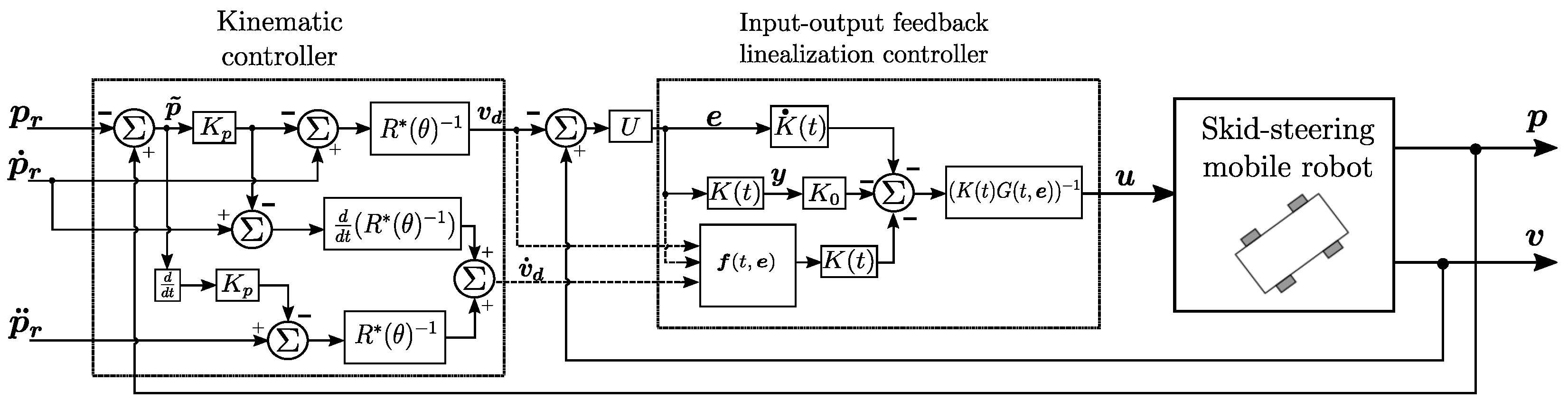
• The proposed control approach consists of a two-level approach. The external control loop (also denoted as kinematic controller) computes the desired velocity for the inner loop and is designed to ensure that the fixed (earth) frame tracking error is bounded. The purpose of the inner control loop is to guarantee that the body frame velocity error is similarly bounded.
• Due to the underactuated nature of the skid-steering mobile robot, the uniform ultimately boundedness of the position error in the earth frame is ensured theoretically without requiring stringent conditions for the desired earth frame trajectories. This statement has been proven to be true by assuming that the desired body velocity produced by the kinematic controller is persistently exciting.
• A simulation study is presented, where the viability of the proposed approach is shown. We test the persistency of the excitation condition resulting from the proposed analysis. Furthermore, a comparison with two known trajectory tracking control schemes is shown. Robustness is tested by using friction coefficients in the vehicle that are position-varying.

The manuscript is organized as follows. Section 2 deals with the model of the mobile robot, the control goal, and the mathematical tools required to prove our main theoretical results. The proposed approach, based on the two loops of feedback and input–output feedback linearization, is provided in Section 3. Simulation results are discussed in Section 4. Finally, the main conclusions from the study and analysis are established in Section 5.

2. Model, Control Goal, and Mathematical Preliminaries

In the next section, the model of a skid-steering mobile robot is presented. Further details are provided in [21,23]. The model corresponds to the free-body diagram depicted in Figure 1.

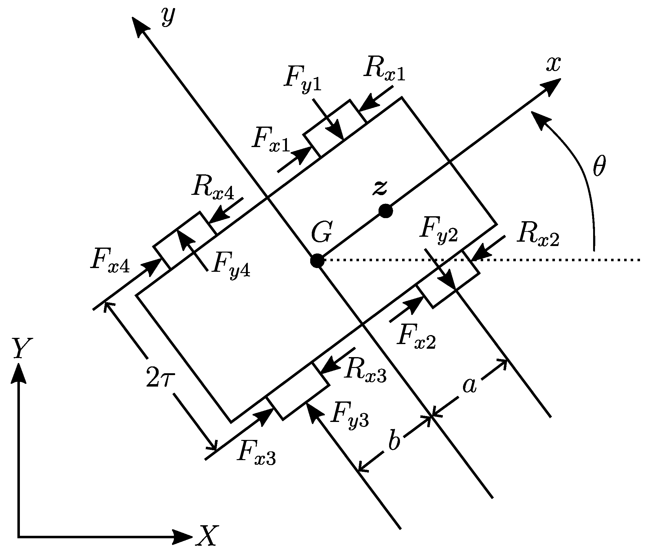
2.1. Model of a Skid-Steering Mobile Robot

Define a fixed reference frame, $F(X,Y)$, and a moving frame, $f(x,y)$, attached to the vehicle body, with origin at the vehicle center of mass G (see Figure 1). The center of mass is located at distances a and b (usually, $a<b$) from the front and rear wheel axes, respectively, and is symmetric with respect to the vehicle sides (at distance $\tau$).

Let us consider the rotation matrices:

$$R\left(\theta \right)=\left[\begin{array}{cc}cos\left(\theta \right)& -sin\left(\theta \right)\\ sin\left(\theta \right)& cos\left(\theta \right)\end{array}\right]$$

and

$$R^{\ast }\left(\theta \right)=\left[\begin{array}{ccc}cos\left(\theta \right)& -sin\left(\theta \right)& 0\\ sin\left(\theta \right)& cos\left(\theta \right)& 0\\ 0& 0& 1\end{array}\right]=\left[\begin{array}{cc}R\left(\theta \right)& 0_{2\times 1}\\ 0_{1\times 2}& 1\end{array}\right].$$

Let $v_x$, $v_y$, $\dot{\theta }=\omega$ be, respectively, the longitudinal, lateral, and angular velocity of the vehicle in frame f. In the fixed frame F, the absolute velocities are

$$\frac{d}{dt}\left[\begin{array}{c}X\\ Y\\ \theta \end{array}\right]=\left[\begin{array}{cc}R\left(\theta \right)& 0_{2\times 1}\\ 0_{1\times 2}& 1\end{array}\right]\left[\begin{array}{c}{v}_x\\ v_y\\ \omega \end{array}\right].$$

(1)

From the differential kinematics (1), we have

$$\left[\begin{array}{c}\dot{X}\\ \dot{Y}\end{array}\right]=R\left(\theta \right)\left[\begin{array}{c}{v}_x\\ v_y\end{array}\right].$$

(2)

For each wheel, $i=1,\cdots ,4$; let $v_{x_i}$ and $v_{y_i}$ be the the longitudinal velocity and the lateral (skidding) velocity, respectively, which are explicitly given by

$$\begin{array}{ccccc}{v}_{x_1}=v_{x_4}& =& v_x-\tau \dot{\theta }& & \left(\mathrm{left}\right)\\ v_{x_2}=v_{x_3}& =& v_x+\tau \dot{\theta }& & \left(\mathrm{right}\right)\\ v_{y_1}=v_{y_2}& =& v_y+a\dot{\theta }& & \left(\mathrm{front}\right)\\ v_{y_3}=v_{y_4}& =& v_y-b\dot{\theta }& & \left(\mathrm{rear}\right).\end{array}$$

(3)

We assume that wheel actuation is equal on each side so as to reduce longitudinal slip. Thus, it will always be $F_{x4}=F_{x1}$ and $F_{x3}=F_{x2}$. Lateral forces, $F_{yi}$, act on the wheels as a consequence of lateral skidding. In addition, a resistive moment, $M_r$, around the center of mass is induced in general by the $F_{yi}$ and $R_{xi}$ forces.

The dynamic model of the skid-steering mobile robot of mass m and inertia J about its center of mass can be rewritten as

$$\begin{array}{ccc}\hfill m{\dot{v}}_x-m{v}_y\omega & =& F_1-R_x\hfill \\ \hfill m{\dot{v}}_y+m{v}_x\omega & =& -F_y\hfill \\ \hfill J\dot{\omega }& =& F_2-M_r,\hfill \end{array}$$

(4)

where $R_x$ and $F_y$ are dissipative forces in the x and y direction of the body frame, respectively, and $M_r$ is the dissipative moment. Furthermore, $F_1$ and $F_2$ are the control inputs.

The longitudinal resistive force is expressed by [21]

$$R_x=f_r\frac{mg}{2}\left(\tanh \left(\beta v_{x_1}\right)+tanh\left(\beta v_{x_2}\right)\right).$$

(5)

The total lateral force is thus

$$F_y=\mu \frac{mg}{a+b}\left(btanh\left(\beta v_{y_1}\right)+atanh\left(\beta v_{y_3}\right)\right),$$

(6)

while the resistive moment is

$$\begin{array}{ccc}\hfill M_r& =& \mu \frac{abmg}{a+b}\left(\tanh \left(\beta v_{y_1}\right)-\tanh \left(\beta v_{y_3}\right)\right)+f_r\frac{\tau mg}{2}\left(\tanh \left(\beta v_{x_2}\right)-\tanh \left(\beta v_{x_1}\right)\right).\hfill \end{array}$$

(7)

It is worth noting that a continuous model of friction has been introduced in the dynamic model (4). This guarantees that the closed-loop system is locally Lipschitz.

2.2. Control Problem Formulation

Let us consider the point of interest given by

$$\mathit{z}=\left[\begin{array}{c}{X}_z\\ Y_z\end{array}\right]=\left[\begin{array}{c}X+d_{0}cos\left(\theta \right)\\ Y+d_{0}sin\left(\theta \right)\end{array}\right],$$

where $d_0$ is constant, such that [21]

$$0<d_0<a.$$

See Figure 1 for an illustration of point z. Thus, the mobile robot pose is defined as

$$\mathit{p}\left(t\right)=\left[\begin{array}{c}{X}_z\left(t\right)\\ Y_z\left(t\right)\\ \theta \left(t\right)\end{array}\right]=\left[\begin{array}{c}\mathit{z}\left(t\right)\\ \theta \left(t\right)\end{array}\right]\in {\mathbb{R}}^3,$$

which is a vector that contains the vehicle position and orientation in the fixed earth frame. Furthermore, the desired point of interest is defined as

$${\mathit{z}}_r\left(t\right)=\left[\begin{array}{c}{X}_{zr}\left(t\right)\\ Y_{zr}\left(t\right)\end{array}\right].$$

Thus, the desired pose is specified by ${\mathit{p}}_r={\left[{\mathit{z}}_r^T{\theta }_r\right]}^T$, with ${\theta }_r=\mathrm{atan}2({\dot{Y}}_{zr}\left(t\right),{\dot{X}}_{zr}\left(t\right))$.

Assumption 1.

The desired pose trajectory, ${\mathit{p}}_r\left(t\right)$, is assumed to be at least twice differentiable. Furthermore,

$${\mathit{p}}_r\left(t\right),{\dot{\mathit{p}}}_r\left(t\right),{\ddot{\mathit{p}}}_r\left(t\right)<\mu ,\forall t\ge 0,$$

with constant $\mu >0$.

Furthermore, the pose error is defined as

$$\tilde{\mathit{p}}=\mathit{p}-{\mathit{p}}_r.$$

(8)

For the sake of simplicity, let us define the control input:

$$\mathit{u}=\left[\begin{array}{c}{F}_1\\ F_2\end{array}\right]=\left[\begin{array}{c}2F_{x1}+2F_{x2}\\ 2\tau (F_{x1}-F_{x2})\end{array}\right].$$

(9)

Thus, the control problem consists of designing a control input, $\mathit{u}\left(t\right)\in {\mathbb{R}}^2$, such that the pose error in the fixed earth frame is uniformly ultimately bounded [38]; that is,

$$∥\tilde{\mathit{p}}\left(t\right)∥\le a_0,\forall t\ge T,$$

(10)

for a compact set of initial conditions, such that

$$∥\tilde{\mathit{p}}\left(0\right)∥\le b_0.$$

(11)

In (10) and (11), the notation $\parallel =\sqrt{{\mathit{x}}^T\mathit{x}}$ stands for the Euclidean norm of vector $\mathit{x}\in {\mathbb{R}}^n$.

2.3. Mathematical Background for Analysis

The following analysis tools are found in the classical textbook [52] and are necessary for the proposed control approach analysis.

Definition 1.

A signal $\varphi :{\mathbb{R}}^{+}\to \mathbb{R}$ is persistently exciting if there exist ${\Delta }_1$, ${\Delta }_2$, and ${\Delta }_3>0$, such that

$${\Delta }_1\ge {\int }_t^{t+{\Delta }_2}\varphi \left(t\right)dt\ge {\Delta }_3, for all t\ge 0.$$

Theorem 1

([52]). Let $\varphi :{\mathbb{R}}^{+}\to \mathbb{R}$ be piecewise continuous. If $\varphi \left(t\right)$ is persistently exciting, then the system is

$$\dot{\eta }\left(t\right)=-\gamma \varphi \left(t\right)\eta \left(t\right),constant \gamma >0,$$

and is globally exponentially stable.

We consider the properties of a so-called perturbed system:

$$\dot{\mathit{x}}=\mathit{f}(t,\mathit{x},\mathit{d}),{\mathit{x}}_0=\mathit{x}\left(0\right),$$

(12)

and relate its properties to those of the unperturbed system:

$$\dot{\mathit{x}}=\mathit{f}(t,\mathit{x},\mathbf{0}),{\mathit{x}}_0=\mathit{x}\left(0\right),$$

(13)

where $t\ge 0$, $\mathit{x}\in {\mathbb{R}}^n$, and $\mathit{d}\in {\mathbb{R}}^m$.

Similarly to [52], we restrict our attention to solution $\mathit{x}\left(t\right)$ and perturbation $\mathit{d}\left(t\right)$ belonging to some arbitrary balls, $B_h\in {\mathbb{R}}^n$ and $B_c\in {\mathbb{R}}^m$.

Consider that the L-∞ norm is defined as

$${\parallel \mathit{x}\parallel }_{\infty }=\underset{i}{sup}\left|x_i\right|.$$

In particular, for $u\left(t\right):{\mathbb{R}}^{+}\to \mathbb{R}$, the notation $u\left(t\right)\in L_{\infty }$ means that ${\left|u\left(t\right)\right|}_{\infty }={sup}_{t\ge 0}\left|u\left(t\right)\right|$ exists.

Theorem 2

([52]). Consider the perturbed system (12) and the unperturbed system (13). Let $\mathit{x}=\mathbf{0}$ be an equilibrium of (13); that is, $\mathit{f}(t,\mathbf{0},\mathbf{0})=\mathbf{0}$ for all $t\ge 0$. Let f be piecewise continuous in t and have continuous and bounded first partial derivatives in x, for all $t\ge 0$, $\mathit{x}\in B_h$, and $\mathit{d}\in B_c$. Let f be Lipschitz in d, with Lipschitz constant $l_d$, for all $t\ge 0$, $\mathit{x}\in B_h$, and $\mathit{d}\in B_c$. Let $\mathit{d}\in L_{\infty }$.

If $\mathit{x}=0$ is the exponentially stable equilibrium point of the unperturbed system, then

(a) 

The perturbed system is small-signal $L_{\infty }$-stable; that is, there exist ${\gamma }_{\infty }$, $c_{\infty }$, such that ${\parallel \mathit{d}\parallel }_{\infty }<c_{\infty }$ implies that

$${\parallel \mathit{x}\parallel }_{\infty }\le {\gamma }_{\infty }{\parallel \mathit{d}\parallel }_{\infty }<h$$

where x is the solution of (12) starting at $\mathit{x}\left(0\right)=\mathbf{0}$.

(b) 

There exists $s\ge 1$, such that, for all $\parallel \mathit{x}\left(0\right)\parallel < h/s$, ${0 < \parallel \mathit{d}\parallel }_{\infty }<c_{\infty }$ implies that $\mathit{x}\left(t\right)$ converges to a $B_{\delta }$ ball of radius $\delta ={\gamma }_{\infty }{\parallel \mathit{d}\parallel }_{\infty }<h$; that is, for all $ϵ>0$ there exists $T\ge 0$, such that

$$\parallel \mathit{x}\parallel <(1+ϵ)\delta$$

for all $t\ge T$, along the solutions of (12) starting at $\mathit{x}\left(0\right)$. In addition, for all $t\ge 0$, $\parallel \mathit{x}\left(t\right)\parallel <h$.

Essentially, Theorem 2 provides sufficient conditions for solution $\mathit{x}\left(t\right)$ of system (12) to be uniformly ultimately bounded [38]. In the textbook [52], Theorems 1 and 2 were used systematically to conclude the robustness of the parameter identification algorithms and adaptive controllers.

3. A Two-Level Control Approach

Once the dynamic model of the skid-steering mobile robot has been defined, we are in position to describe and present the corresponding analysis of the proposed control approach. The adopted scheme is described as two-level control architecture and also denoted as nested control: an external kinematic control and an inner input–output feedback linearization control loop. Figure 2 illustrates the proposed control approach, which relies on the described two-level architecture. Further details are given in the next section.

3.1. Outer Control Loop: Kinematic Control

The kinematic control loop will be defined in this subsection. Kinematic control considers the differential relationship (1) as the mobile robot model, the body frame velocity vector,

$$\mathit{v}={\left[\begin{array}{c}{v}_x\\ v_y\\ \omega \end{array}\right]}^T\in {\mathbb{R}}^3,$$

(14)

being the input of the mobile robot, while the pose, p, is the variable of interest.

Motivated by the motion rate control [53,54], let us definite the desired body frame velocity as

$${\mathit{v}}_d=\left[\begin{array}{c}{v}_{xd}\\ v_{yd}\\ {\omega }_d\end{array}\right]=R^{\ast }{\left(\theta \right)}^{-1}\left[{\dot{\mathit{p}}}_r-K_p\tilde{\mathit{p}}\right],$$

(15)

where $K_p$ is a $3\times 3$ symmetric positive definite matrix, and the tracking error, $\tilde{\mathit{p}}$, is defined in (8). Equation (15) also denotes the outer control loop.

Let us define the following error signals:

$$\begin{array}{ccc}\hfill e_1& =& v_x-v_{xd},\hfill \\ \hfill e_2& =& \omega -{\omega }_d,\hfill \\ \hfill e_3& =& v_y-v_{yd},\hfill \end{array}$$

(16)

which can be placed into a vector:

$$\mathit{e}=\left[\begin{array}{c}{e}_1\\ e_3\\ e_2\end{array}\right].$$

The reason for defining the velocity error as in (16) is because the velocity in $v_x\left(t\right)$ is related to the applied force, $F_1\left(t\right)$, and the $\omega \left(t\right)$ is related to the applied torque, $F_2\left(t\right)$. This will facilitate the derivation of the input–output linearization controller. In order to balance the relation between the body frame velocity error, $\mathit{e}\left(t\right)$, and the velocity error vector in the fixed frame, $\dot{\tilde{\mathit{p}}}\left(t\right)$, the matrix

$$U=\left[\begin{array}{ccc}1& 0& 0\\ 0& 0& 1\\ 0& 1& 0\end{array}\right]$$

is defined.

The kinematic relation (2) can be rewritten as

$$\dot{\tilde{\mathit{p}}}=-{\dot{\mathit{p}}}_r+R^{\ast }\left(\theta \right)U\mathit{e}+R^{\ast }\left(\theta \right)\left[\begin{array}{c}{v}_{xd}\\ v_{yd}\\ {\omega }_d\end{array}\right].$$

(17)

By substituting (15) into the error system (17), the expression

$$\dot{\tilde{\mathit{p}}}=-K_p\tilde{\mathit{p}}+R^{\ast }\left(\theta \right)U\mathit{e}$$

(18)

is obtained.

Provided that the body frame velocity error, $\mathit{e}\left(t\right)$, is a uniformly bounded signal, one can expect that the pose error, $\tilde{\mathit{p}}\left(t\right)$, will satisfy the control objectives in (10) and (11). This claim will be precisely proven next by means of the introduction of an input–output linearization controller, $\mathit{u}\left(t\right)$.

As seen in Figure 2, the inputs for the inner control loop are the desired body frame velocity, ${\mathit{v}}_d\left(t\right)$, in (15), its time derivative,

$${\dot{\mathit{v}}}_d\left(t\right)=R^{\ast }{\left(\theta \right)}^{-1}\left[{\ddot{\mathit{p}}}_r-K_p\dot{\tilde{\mathit{p}}}\right]+\left[\frac{d}{dt}{R}^{\ast }{\left(\theta \right)}^{-1}\right]\left[{\dot{\mathit{p}}}_r-K_p\tilde{\mathit{p}}\right],$$

and the actual body frame velocity, $\mathit{v}\left(t\right)\in {\mathbb{R}}^3$.

An important observation is that, thanks to Assumption 1, for all $\theta \in \mathbb{R}$, the matrix $R^{\ast }\left(\theta \right)$ is invertible and bounded, and for all $\tilde{\mathit{p}}$, $\dot{\tilde{\mathit{p}}}$ $\in B_p$, with $B_p\subset {\mathbb{R}}^3$, a compact set that contains the origin, the body frame desired velocity and acceleration ${\mathit{v}}_d\left(t\right)$, and ${\dot{\mathit{v}}}_d\left(t\right)$, respectively, are bounded for all time $t\ge 0$.

3.2. Inner Control Loop: Input–Output Linearization

In this subsection, a controller, $\mathit{u}\left(t\right)$, will be developed with the aim of ensuring the uniform ultimately boundedness of the body frame velocity error, $\mathit{e}\left(t\right)$; that is,

$$∥\mathit{e}\left(t\right)∥\le a_{v0},\forall t\ge T, \mathrm{with} T\ge 0,$$

(19)

where $\mathit{e}\left(t\right)$ is defined in (16), for $\mathit{e}\left(0\right)\in S$, where $S\subset {\mathbb{R}}^3$ is a compact set.

In order to derive the inner-loop controller, we follow the procedure described in textbook [37], and the works [50,55], for designing an input–output linearization controller.

3.2.1. Error System Development

Our goal is to developed an error system for which an input–output linearization approach will be applied.

The time derivative of the error signals (16) is computed by using the skid-steering mobile robot model (4), as follows:

$$\begin{array}{ccc}\hfill \frac{d}{dt}{e}_1& =& (e_3+v_{yd})(e_2+{\omega }_d)+\frac{F_1}{m}-\frac{R_x}{m}-{\dot{v}}_{xd},\hfill \\ \hfill \frac{d}{dt}{e}_2& =& -\frac{M_r}{J}+\frac{F_2}{J}-{\dot{\omega }}_d,\hfill \\ \hfill \frac{d}{dt}{e}_3& =& -(e_1+v_{xd})(e_2+{\omega }_d)-\frac{F_y}{m}-{\dot{v}}_{yd},\hfill \end{array}$$

which can be written in the compact standard form

$$\frac{d}{dt}\mathit{e}=\mathit{f}(t,\mathit{e})+G(t,\mathit{e})\mathit{u},$$

(20)

where

$$\mathit{f}(t,\mathit{e})=\left[\begin{array}{c}(e_3+v_{yd})(e_2+{\omega }_d)-\frac{R_x}{m}-{\dot{v}}_{xd}\\ -\frac{M_r}{J}-{\dot{\omega }}_d\\ -(e_1+v_{xd})(e_2+{\omega }_d)-\frac{F_y}{m}-{\dot{v}}_{yd}\end{array}\right],$$

(21)

$$G(t,\mathit{e})=\left[\begin{array}{cc}1/m& 0\\ 0& 1/J\\ 0& 0\end{array}\right],$$

and u defined in (9).

3.2.2. Input–Output Linearization Design

As highlighted in [37], the input–output methodology consists of defining an output function, $\mathit{y}\left(\mathit{e}\right)$. The definition of the output function shall be carried out to facilitate the analysis of the internal dynamics. With this in mind, the following output function is defined:

$$\mathit{y}=K\left(t\right)\mathit{e},$$

(22)

where $K\left(t\right)\in {\mathbb{R}}^{2\times 3}$ is a time-varying matrix; that is,

$$K\left(t\right)=\left[\begin{array}{ccc}{k}_{11}\left(t\right)& k_{12}\left(t\right)& k_{13}\left(t\right)\\ k_{21}\left(t\right)& k_{22}\left(t\right)& k_{23}\left(t\right)\end{array}\right].$$

(23)

The gain $k_{ij}\left(t\right)$ will be defined so that the solutions of the internal dynamics are uniformly ultimately bounded. The selection of the gain $k_{ij}\left(t\right)$ will be presented in a constructive form.

The reasons to define the output function, y, as a linear combination of the velocity error, e, is to facilitate the analysis of the internal dynamics; see also the papers [50,55], where a similar idea was used for the control of a Furuta pendulum and a flexible joint robot, respectively.

Once we have written the error system in the standard form and defined the output function, the next step is to differentiate each component of the output function $r_i$ times for the control input to appear. Thus, the time derivative of the output function, y, is given:

$$\dot{\mathit{y}}=\dot{K}\mathit{e}+K\dot{\mathit{e}}=\dot{K}\mathit{e}+K\mathit{f}(t,\mathit{e})+KG(t,\mathit{e})\mathit{u}.$$

(24)

The total relative degree is $r=r_1+r_2=1+1=2$, since the output function, y, has dimension 2 and the control input appears after differentiating with respect to times $y_1$ and $y_2$; see [37], p. 267, for further discussions.

What follows is the method to find a relationship between the controller, $\mathit{u}\left(t\right)$, and the dynamics of the output function, $\mathit{y}\left(t\right)$. As suggested in [37], one should select $\mathit{u}\left(t\right)$ to cancel the nonlinearities of (24) and guarantee the tracking convergence of $\mathit{y}\left(t\right)$. Specifically, the control input that linearizes the dynamics of $\mathit{y}\left(t\right)$ is given by

$$\mathit{u}={\left[KG(t,\mathit{e})\right]}^{-1}[-K\mathit{f}(t,\mathit{e})-\dot{K}\mathit{e}-K_0\mathit{y}],$$

(25)

with $K_0=K_0^T>0$; that is, $K_0\in {\mathbb{R}}^{2\times 2}$ is a symmetric positive definite matrix. By substituting the control action (25) into the output dynamics (24), we obtain

$$\dot{\mathit{y}}=-K_0\mathit{y}.$$

(26)

It is possible to show that $\mathit{y}\left(t\right)\to \mathbf{0}$ as $t\to \infty$ with exponential convergence rate.

Notice that the control action, u, in (25) depends on the expression ${\left[KG(t,\mathit{e})\right]}^{-1}$, which should hold for all time $t\ge 0$ and $\mathit{e}\in {\mathbb{R}}^3$. In other words, the square product matrix, $KG(t,\mathit{e})$, should be invertible. In order to guarantee that $KG(t,\mathit{e})$ is invertible and the indetermination of the control action, u, the following condition should be satisfied:

$$det\left(KG(t,\mathit{e})\right)=\frac{1}{mJ}\left[k_{11}{k}_{22}-k_{12}{k}_{21}\right]\ne 0.$$

(27)

Equation (26) denotes the external dynamics. The next step is to compute the internal dynamics. With this aim, let us define the change of variable $\eta \left(\mathit{e}\right)$, such that [37]

$$\frac{\partial \eta \left(\mathit{e}\right)}{\partial \mathit{e}}G(t,\mathit{e})=\left[\begin{array}{c}00\end{array}\right].$$

(28)

A selection is

$$\eta \left(\mathit{e}\right)=e_3,$$

so that the evaluation of Equation (28) results in

$$\left[\begin{array}{ccc}0& 0& 1\end{array}\right]\left[\begin{array}{cc}1/m& 0\\ 0& 1/J\\ 0& 0\end{array}\right]=\left[\begin{array}{c}00\end{array}\right].$$

(29)

To compute the internal dynamics, the following transformation is defined:

$$\left[\begin{array}{c}\eta \\ y_1\\ y_2\end{array}\right]=\underset{H}{\underbrace{\left[\begin{array}{ccc}0& 0& 1\\ k_{11}& k_{12}& k_{13}\\ k_{21}& k_{22}& k_{23}\end{array}\right]}}\left[\begin{array}{c}{e}_1\\ e_2\\ e_3\end{array}\right].$$

(30)

Then, the inverse relation of (30) is given by

$$\left[\begin{array}{c}{e}_1\\ e_2\\ e_3\end{array}\right]=\underset{H^{-1}}{\underbrace{\left[\begin{array}{ccc}\frac{k_{12}{k}_{23}-k_{13}{k}_{22}}{k_{11}{k}_{22}-k_{12}{k}_{21}}& \frac{k_{22}}{k_{11}{k}_{22}-k_{12}{k}_{21}}& -\frac{k_{12}}{k_{11}{k}_{22}-k_{12}{k}_{21}}\\ -\frac{k_{11}{k}_{23}-k_{13}{k}_{21}}{k_{11}{k}_{22}-k_{12}{k}_{21}}& -\frac{k_{21}}{k_{11}{k}_{22}-k_{12}{k}_{21}}& \frac{k_{11}}{k_{11}{k}_{22}-k_{12}{k}_{21}}\\ 1& 0& 0\end{array}\right]}}\left[\begin{array}{c}\eta \\ y_1\\ y_2\end{array}\right].$$

(31)

It is worth noting that (31) holds if

$$det\left(H\right)=k_{11}{k}_{22}-k_{12}{k}_{21}\ne 0,$$

which correspond to the invertibility condition (27) of the matrix $KG(t,\mathit{e})$.

For the sake of simplicity, we will adopt the notation

$$H^{-1}=\left[\begin{array}{ccc}{c}_{11}& c_{12}& c_{13}\\ c_{21}& c_{22}& c_{23}\\ 1& 0& 0\end{array}\right]=\left[\begin{array}{ccc}\frac{k_{12}{k}_{23}-k_{13}{k}_{22}}{k_{11}{k}_{22}-k_{12}{k}_{21}}& \frac{k_{22}}{k_{11}{k}_{22}-k_{12}{k}_{21}}& -\frac{k_{12}}{k_{11}{k}_{22}-k_{12}{k}_{21}}\\ -\frac{k_{11}{k}_{23}-k_{13}{k}_{21}}{k_{11}{k}_{22}-k_{12}{k}_{21}}& -\frac{k_{21}}{k_{11}{k}_{22}-k_{12}{k}_{21}}& \frac{k_{11}}{k_{11}{k}_{22}-k_{12}{k}_{21}}\\ 1& 0& 0\end{array}\right]$$

(32)

to make the calculations shown in the next section more compact.

By using (31), we are in position to compute the internal dynamics as follows:

$$\frac{d}{dt}\eta ={\dot{e}}_3=-e_1{e}_2-v_{xd}{e}_2-{\omega }_d{e}_1-v_{xd}{\omega }_d-\frac{F_y}{m}-{\dot{v}}_{yd}.$$

(33)

Substituting the expressions of $e_1$ and $e_2$ from (31) into (33), we have

$$\begin{array}{ccc}\hfill \frac{d}{dt}\eta & =& -\left(c_{11}\eta +c_{12}{y}_1+c_{13}{y}_2\right)\left(c_{21}\eta +c_{22}{y}_1+c_{23}{y}_2\right)\hfill \\ & & -v_{xd}\left(c_{21}\eta +c_{22}{y}_1+c_{23}{y}_2\right)-{\omega }_d\left(c_{11}\eta +c_{12}{y}_1+c_{13}{y}_2\right)\hfill \\ & & -v_{xd}{\omega }_d-\frac{F_y}{m}-{\dot{v}}_{yd}.\hfill \end{array}$$

(34)

The system (34) can be written with the structure suggested in [55] as follows:

$$\frac{d}{dt}\eta =f_0(t,\eta )+\Phi (t,\eta ,\mathit{y})+d_0,$$

(35)

where

$$\begin{array}{ccc}\hfill f_0(t,\eta )& =& -(v_{xd}{c}_{21}+{\omega }_d{c}_{11})\eta -c_{11}{c}_{21}{\eta }^2,\hfill \end{array}$$

(36)

$$\begin{array}{ccc}\hfill {\Phi }_0(t,\eta ,\mathit{y})& =& -c_{11}\eta (c_{22}{y}_1+c_{23}{y}_2)-c_{21}\eta (c_{12}{y}_1+c_{13}{y}_2)\hfill \end{array}$$

(37)

$$\begin{array}{ccc}& & -(c_{12}{y}_1+c_{13}{y}_2)(c_{22}{y}_1+c_{23}{y}_2)\hfill \end{array}$$

(38)

$$\begin{array}{ccc}& & -v_{xd}\left(c_{22}{y}_1+c_{23}{y}_2\right)-{\omega }_d\left(c_{12}{y}_1+c_{13}{y}_2\right)\hfill \end{array}$$

(39)

$$\begin{array}{ccc}\hfill d_0& =& -v_{xd}{\omega }_d-\frac{F_y}{m}-{\dot{v}}_{yd}.\hfill \end{array}$$

(40)

It is worth noting that, at $\mathit{y}=0$, the function

$${\Phi }_0(t,\eta ,\mathbf{0})=0,\forall t\ge 0,\eta \in \mathbb{R}.$$

Thus, by continuity of the function ${\Phi }_0(t,\eta ,\mathit{y})$, and assuming that $\eta \left(t\right)$ is uniformly continuous, we have

$${\Phi }_0(t,\eta \left(t\right),\mathit{y}\left(t\right))\to 0 as \mathit{y}\left(t\right)\to \left[\begin{array}{c}0\\ 0\end{array}\right].$$

The signals $v_{xd}\left(t\right)$, $v_{xd}\left(t\right)$, and ${\omega }_d\left(t\right)$, and their respective time-derivatives ${\dot{v}}_{xd}\left(t\right)$, ${\dot{v}}_{xd}\left(t\right)$, and ${\dot{\omega }}_d\left(t\right)$, are generated by the output of the kinematic (outer) controller (15). Furthermore, ${\dot{v}}_{xd}\left(t\right)$, ${\dot{v}}_{xd}\left(t\right)$, and ${\dot{\omega }}_d\left(t\right)$ depend on the actual pose, $\mathit{p}\left(t\right)$, and the desired one, ${\mathit{p}}_r\left(t\right)$.

By definition, the friction forces and moments $R_x$, $F_y$, and $M_r$ are bounded for all time. This is immediately deduced from the definition of the dissipative forces and moments $R_x$, $F_y$, and $M_r$ given in Equations (5)–(7), respectively.

Once we have defined the above-written framework, the following results are stated. Section 2.3 shows the definition of a persisting exciting signal as well as the required analysis tools to prove our main results.

Proposition 1.

Assume that the disturbance term $d_0$ in (40) is null for all time $t\ge 0$; that is,

$$d_0\left(t\right)=0,\forall t\ge 0.$$

(41)

Consider that

$$\begin{array}{ccc}{k}_{11}& >& 0,\hfill \\ k_{22}& >& 0,\hfill \\ k_{12}& =& -k_{21},\hfill \\ k_{13}& =& {\alpha }_2{k}_{21}{v}_{xd}-{\alpha }_1{k}_{11}{\omega }_d,\hfill \\ k_{23}& =& -{\alpha }_1{k}_{21}{\omega }_d-{\alpha }_2{k}_{22}{v}_{xd}.\hfill \end{array}$$

(42)

The constants ${\alpha }_1$ and ${\alpha }_2$ are selected either as strictly positive, or one of them is zero and the another is strictly positive. Furthermore, consider that

$$\varphi ={\alpha }_1{\omega }_d^2+{\alpha }_2{v}_{xd}^2$$

(43)

is a persisting exciting signal. Then, the vector ${\left[\eta \left(t\right)\mathit{y}{\left(t\right)}^T\right]}^T\in {\mathbb{R}}^n$ converges to zero exponentially, provided that the initial conditions start as a compact set.

Proof. 

Under assumption (41), the internal and external dynamics can be written as

$$\begin{array}{ccc}\hfill \frac{d}{dt}\mathit{y}& =& -K_o\mathit{y},\hfill \end{array}$$

(44)

$$\begin{array}{ccc}\hfill \frac{d}{dt}\eta & =& f_0(t,\eta )+\Phi (t,\eta ,\mathit{y}),\hfill \end{array}$$

(45)

which has an equilibrium point at $\eta =0$ and $\mathit{y}=\mathbf{0}$.

The zero dynamics is given by

$$\frac{d}{dt}\eta =f_0(t,\eta )+\Phi (t,\eta ,\mathbf{0}),$$

which can be linearized around $\eta =0$, resulting in

$$\frac{d}{dt}\eta \left(t\right)=\left[-{\omega }_d\left(\frac{k_{12}{k}_{23}-k_{13}{k}_{22}}{k_{11}{k}_{22}-k_{12}{k}_{21}}\right)+v_{xd}\left(\frac{k_{11}{k}_{23}-k_{13}{k}_{21}}{k_{11}{k}_{22}-k_{12}{k}_{21}}\right)\right]\eta \left(t\right),$$

(46)

where the explicit definitions of element $c_{ij}$ of the matrix $H^{-1}$ in (32) were used.

By substituting the gains selection (42) into Equation (46), and after some algebra, we obtain

$$\frac{d}{dt}\eta \left(t\right)=-\varphi \left(t\right)\eta \left(t\right),$$

with $\varphi \left(t\right)$ defined in (43). Since $\varphi \left(t\right)$ is a persisting exciting signal, the local exponential convergence of $\eta \left(t\right)$ can be claimed by Theorem 1. Since $K_0$ is a symmetric positive definite matrix, the local exponential stability of the state-space origin of (44) and (45) is concluded by using arguments of cascade systems [56], and thus Proposition 1 is proven. □

Proposition 2.

Assume that the control gains satisfy the conditions expressed in (42) and that $\varphi \left(t\right)$ in (43) is a persistently exciting signal. Then, the solutions $\mathit{y}\left(t\right)$ and $\eta \left(t\right)$ of the external and internal dynamics in (26) and (35), respectively, are uniformly ultimately bounded.

Proof. 

By defining

$$\mathit{d}\left(t\right)=\left[\begin{array}{c}\mathit{y}\left(t\right)\\ d_0\left(t\right)\end{array}\right],$$

the internal dynamics (35) have the same structure as the nonlinear system (12). For $d_0=0$, the control gains satisfying (42) and $\varphi \left(t\right)$ in (43) are assumed to be a persistently exciting signal; the local exponential stability of the internal dynamics was proven in Proposition 1.

Furthermore, since $\mathit{y}\left(t\right)$ converges to zero exponentially and $d_0\left(t\right)$ is bounded for all time, we have

$${\left|\right|\mathit{d}\left(t\right)\parallel }_{\infty }\le c_{\infty }.$$

Since all the conditions of Theorem 2 are satisfied, the solution $\eta \left(t\right)$ converges to a ball, $B_{\delta }$, of radius $\delta ={\gamma }_{\infty }{\parallel \mathit{d}\parallel }_{\infty }<h$. In other words, for all $ϵ>0$, there exists $T\ge 0$, such that

$$\left|\eta \right|<(1+ϵ)\delta$$

for all $t\ge T$, which means at the same time that $\eta \left(t\right)$ is a uniformly ultimately bounded signal. □

It is worth noting that the control law, $\mathit{u}\left(t\right)$, in (25) requires the time derivative of the control gain, $K\left(t\right)$. Thus, with the given design in Propositions 1 and 2, we have

$$\frac{d}{dt}K\left(t\right)=\left[\begin{array}{ccc}0& 0& {\alpha }_2{k}_{21}{\dot{v}}_{xd}-{\alpha }_1{k}_{11}{\dot{\omega }}_d\\ 0& 0& -{\alpha }_1{k}_{21}{\dot{\omega }}_d-{\alpha }_2{k}_{22}{\dot{v}}_{xd}\end{array}\right].$$

Finally, by means of relation (31), we can see that

$${\parallel \mathit{e}\left(t\right)\parallel \le \parallel H\left(t\right)}^{-1}\parallel ∥\left[\begin{array}{c}\eta \left(t\right)\\ \mathit{y}\left(t\right)\end{array}\right]∥$$

is satisfied for all time $t\ge 0$. In consequence, the error signal, $\mathit{e}\left(t\right)$, is uniformly ultimately bounded and inequality (19) is satisfied.

3.3. Bounding of the Pose Error

We have used the kinematic controller, ${\mathit{v}}_d\left(t\right)$, in (15) in the outer loop and the body frame velocity controller, $\mathit{u}\left(t\right)$, in (25) in the inner loop. We have proven that $\mathit{u}\left(t\right)$ (25) ensures that the body frame velocity error, $\mathit{e}\left(t\right)$, is a uniformly bounded signal. The final step is to show with the given control law that the control goal established in inequalities (10) and (11) is attained.

Proposition 3.

The pose error (the position error in fixed earth coordinates), $\tilde{\mathit{p}}\left(t\right)$, is a uniformly ultimately bounded signal; that is, $\tilde{\mathit{p}}\left(t\right)$ satisfies inequalities (10) and (11) established as the control goal.

Proof. 

The proof is similar to the proofs of Propositions 1 and 2. The fist step is to show that the equilibrium point, $\tilde{\mathit{p}}=0$, of the system

$$\dot{\tilde{\mathit{p}}}=-K_p\tilde{\mathit{p}}$$

is globally exponentially stable. The second step is that by defining

$$\mathit{d}\left(t\right)=R^{\ast }\left(\theta \left(t\right)\right)U\mathit{e}\left(t\right),$$

system (18) has the same structure as system (12). Since ${\parallel \mathit{d}\left(t\right)\parallel }_{\infty }\le c_{\infty }$ and all conditions of Theorem 2 are satisfied, the solution $\tilde{\mathit{p}}\left(t\right)$ is uniformly ultimately bounded. □

Proposition 1 establishes that in the absence of the perturbation $d_0\left(t\right)$ and under the condition persistency of excitation of the the signal $\varphi \left(t\right)$, which is a function of the desired signals $v_{xd}\left(t\right)$ and ${\omega }_d\left(t\right)$, the limit

$$\underset{t\to \infty }{lim}\eta \left(t\right)=\underset{t\to \infty }{lim}{e}_3\left(t\right)=\underset{t\to \infty }{lim}[v_y\left(t\right)-v_{yd}\left(t\right)]=0$$

will be satisfied with exponential convergence rate. Thus, from Definition 1 and Theorem 1 given in the mathematical background of Section 2.3, one can expect that the larger the energy of the signal, $\varphi \left(t\right)$, the faster the convergence of the velocity error, $e_3\left(t\right)$. In Proposition 2, where the perturbation, $d_0\left(t\right)$, is taken into account, the most we can say is that the error, $e_3\left(t\right)$, is uniformly ultimately bounded, no matter the amount of energy contained by the signal, $\varphi \left(t\right)$. Based on the previous discussion, we can still conjecture that the velocity error in the body frame, $\mathit{e}\left(t\right)$, and the position error in the fixed frame, $\tilde{\mathit{p}}\left(t\right)$, will be reduced if the energy of the signal, $\varphi \left(t\right)$, increases. This will be verified numerically in the following section.

4. Simulation Results

In this section, the numerical simulation results are presented. The following set of simulations are presented:

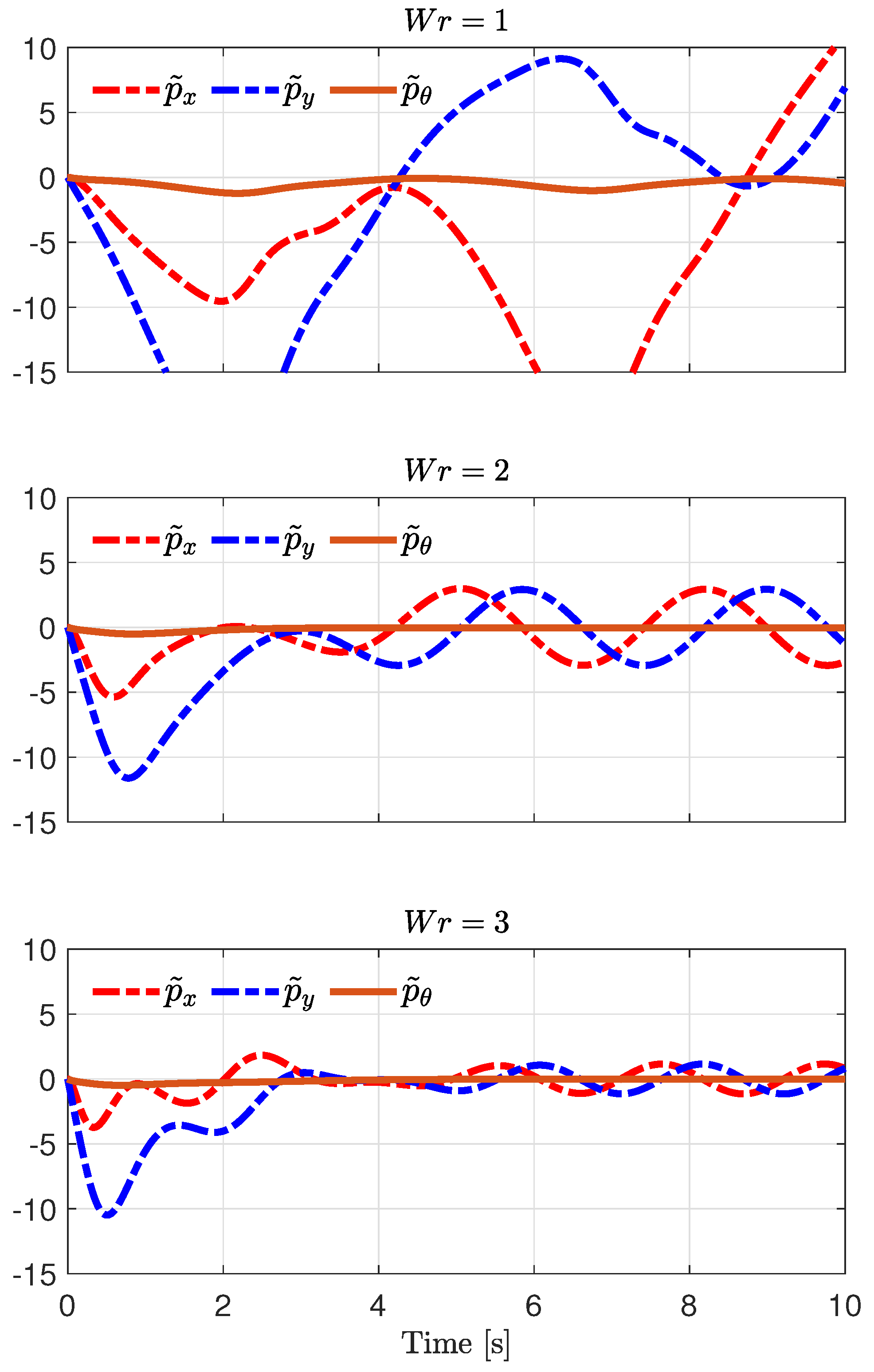
• A simulation set with the proposed input–output linearization controller using a trajectory that draws a circular path in earth coordinates at three different speeds. This test is useful to verify the conjecture that the larger the energy of the desired trajectory, the smaller the tracking error, and that is intuitively derived from Propositions 1 and 2.
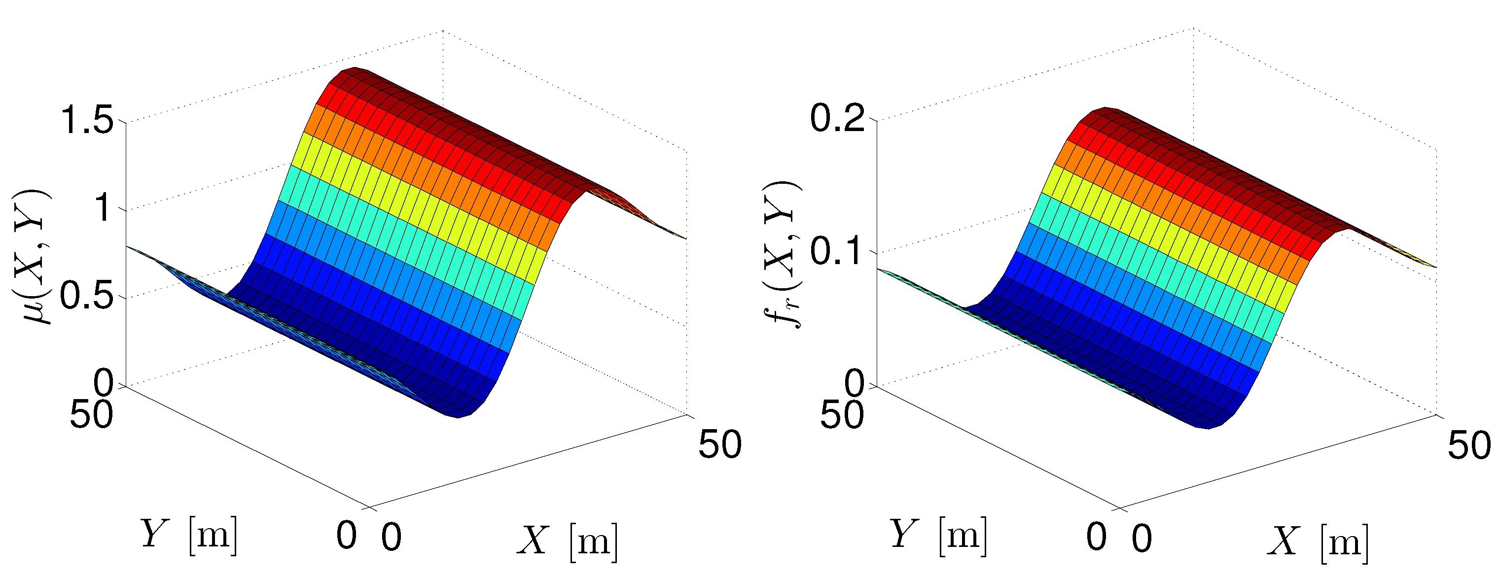
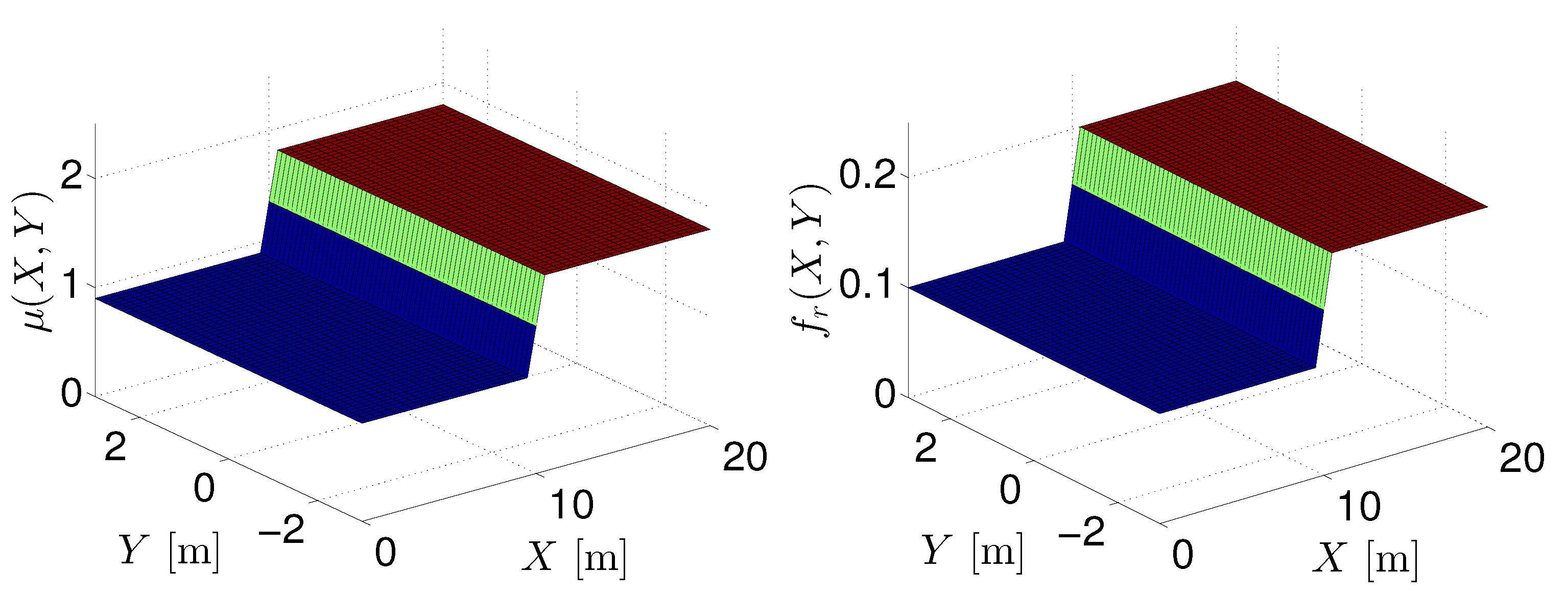
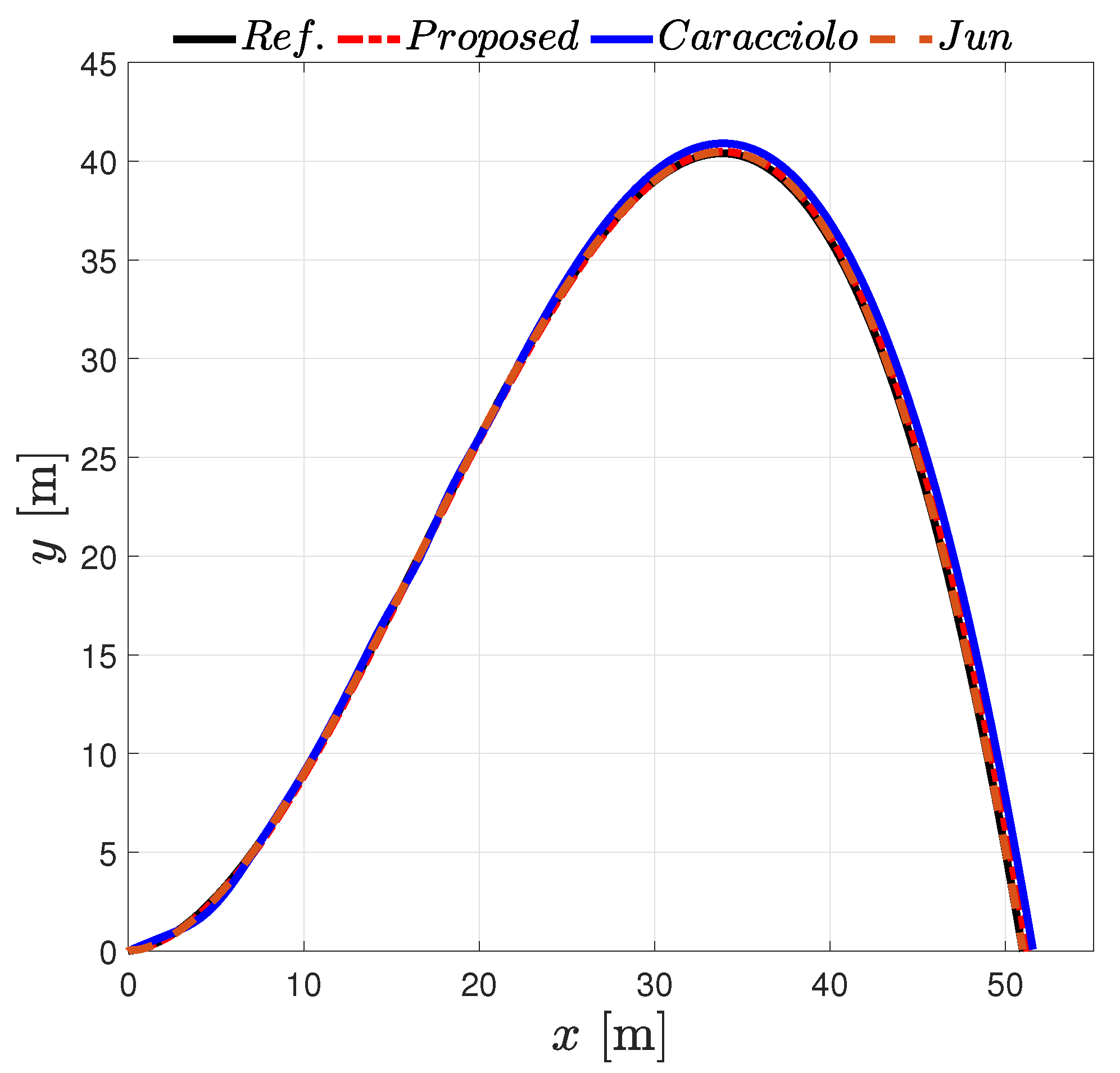
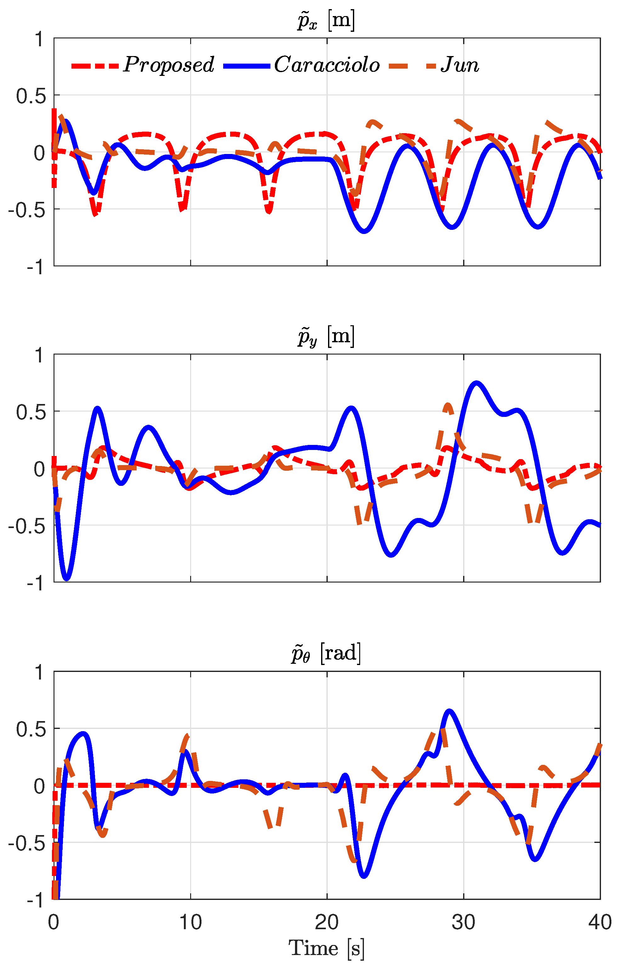
• A simulation set comparing the proposed input–output linearization controller with respect to another two known trajectory tracking control schemes. We consider a polynomial path in earth coordinates and continuous changes in the vehicle friction parameters so that continuous changes in the characteristics of the terrain are obtained.
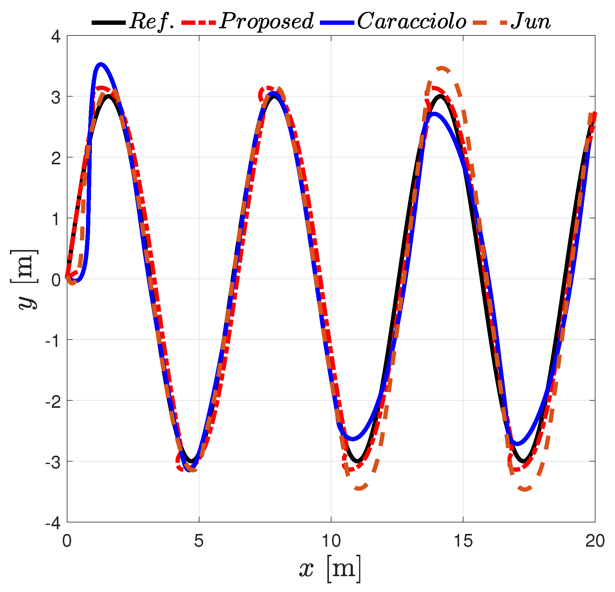
• The third simulation set is similar to the second one but a path that draws a sine wave in earth coordinates and a discontinuous change in the vehicle friction parameters are used.

The parameters of the ATRV-2 robot have been used [21]. Specifically, $a=0.37$ (m), $b=0.55$ (m), 2$\tau$ = 0.63 (m), and wheel radius $r=0.2$ (m). The vehicle mass is $m=116$ (kg) and its inertia is $J=20$ (kg m${}^3$). We used $d_0=0.18$ (m) as the coordinate of the point of interest, z. A value of $\beta =100$ in the resistive forces and moment (5)–(7) has been selected. As mentioned earlier, we have used fixed values of $\mu$ and $f_r$ in the vehicle for the first set of simulations, and varying values of $\mu (X,Y)$ and $f_r(X,Y)$ in the vehicle for the second and third sets of simulations. Details will be provided in the coming discussions.

4.1. Tracking a Circular Path at Different Speeds

We begin the numerical simulation discussions with a test that consists of showing the sensibility of the tracking error, $\tilde{\mathit{p}}\left(t\right)$, to the persistency of the excitation condition of the controller. The following desired path is defined:

$${\mathit{z}}_r\left(t\right)=\left[\begin{array}{c}{X}_{zr}\left(t\right)\\ Y_{zr}\left(t\right)\end{array}\right]=\left[\begin{array}{c}{r}_{c}cos\left(W_{r}t\right)\\ r_{c}sin\left(W_{r}t\right)\end{array}\right]\left[\mathrm{m}\right].$$

With ${\theta }_r=W_{r}t$, the desired pose, ${\mathit{p}}_r\left(t\right)={\left[{\mathit{z}}_r{\left(t\right)}^T{\theta }_r\left(t\right)\right]}^T$, is obtained. Three simulations were carried out by using $W_r=1$, 2, and 3 (rad/s), while $r_c=10$ (m) was used. The selected gains are

$$\begin{array}{ccc}\hfill K_p& =& diag\{1,1,1\},\hfill \\ \hfill K_0& =& diag\{2,2,2\},\hfill \end{array}$$

where ${\alpha }_1=1$, ${\alpha }_2=0.01$, $k_{11}=100$, $k_{12}=1$, $k_{21}=-k_{12}$, $k_{22}=k_{11}$, $k_{13}$, and $k_{23}$ are indicated in Proposition 2. In these simulations, the initial conditions are $X\left(0\right)=10$ (m), $Y\left(0\right)=10$ (m), $\theta \left(0\right)=0$ (rad), $v_x\left(0\right)=0$ (m/s), $v_y\left(0\right)=0$ (m/s), and $\omega \left(0\right)=0$ (rad/s). The friction parameters $\mu =0.9$ and $f_r=0.1$ were used in both the vehicle and the controller.

Figure 3 describes the path drawn by the vehicle in each one of the simulations. Furthermore, in Figure 4 the time evolution of tracking errors ${\tilde{p}}_x\left(t\right)=X_z\left(t\right)-X_{zr}\left(t\right)$, ${\tilde{p}}_y\left(t\right)=Y_z\left(t\right)-Y_{zr}\left(t\right)$, and ${\tilde{p}}_{\theta }\left(t\right)=\theta \left(t\right)-{\theta }_r\left(t\right)$ can be appreciated. Clearly, the larger the value of the path frequency, $W_r$, the smaller the pose error, $\tilde{\mathit{p}}\left(t\right)$. In other words, the trajectory tracking error decreases as the value of $W_r$ increases. The root mean squared (RMS) value of the components of the pose error vector, $\tilde{\mathit{p}}\left(t\right)$, has been computed for each one of the simulations. The obtained RMS values are given in

Table 1. Proposed input–output linearization controller: RMS values of the trajectory tracking errors ${\tilde{p}}_x\left(t\right)=X_z\left(t\right)-X_{zr}\left(t\right)$, ${\tilde{p}}_y\left(t\right)=Y_z\left(t\right)-Y_{zr}\left(t\right)$, and ${\tilde{p}}_{\theta }\left(t\right)=\theta \left(t\right)-{\theta }_r\left(t\right)$ for $W_r=1$, 2, and 3 (rad/s). Percentage of improvement is computed with respect to the RMS value obtained with $W_r=1$ (rad/s).

$\tilde{\mathit{p}}$	${\mathit{W}}_{\mathit{r}}=1$	${\mathit{W}}_{\mathit{r}}=2$	%	${\mathit{W}}_{\mathit{r}}=3$	%
${\tilde{p}}_x$	8.8907	2.1699	75.59	1.0887	87.75
${\tilde{p}}_y$	9.7074	3.9841	58.95	2.9552	69.55
$\tilde{\theta }$	0.6042	0.1787	70.42	0.1858	69.24

and they corroborate the fact that tracking errors decrease as the value of $W_r$ increases. We have confirmed numerically that the closed-loop system is stable for a trajectory of ${\mathit{z}}_d\left(t\right)$, such that $\varphi \left(t\right)$ in (43) is persistently exciting.

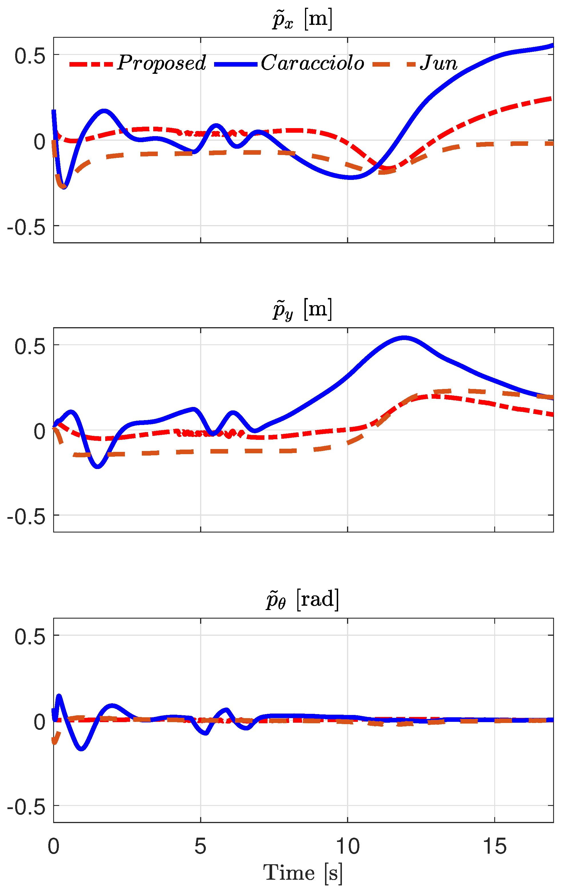
4.2. Comparison with the Controllers [21,31]: Polynomial Path

A dynamic feedback linearization was introduced by Caracciolo et al. [21]. The controller given there corresponds to a dynamic feedback linearization algorithm. Furthermore, Jun et al. [31] proposed a controller using a backstepping technique that guarantees the Lyapunov stability. The controllers reported in [21,31] have been numerically simulated in order to compare their performance with respect to the controller introduced in this paper.

Let us consider the path given by

$${\mathit{z}}_r\left(t\right)=\left[\begin{array}{c}{X}_{zr}\left(t\right)\\ Y_{zr}\left(t\right)\end{array}\right]=\left[\begin{array}{c}3t\\ -0.018t^3+0.3t^2+0.3t\end{array}\right]\left[\mathrm{m}\right].$$

The desired pose is specified by ${\mathit{p}}_r\left(t\right)={\left[{\mathit{z}}_r{\left(t\right)}^T{\theta }_r\left(t\right)\right]}^T$, where ${\theta }_r=\mathrm{atan}2({\dot{Y}}_{zr},{\dot{X}}_{zr})$. The resulting desired pose is used to numerically simulate the Caracciolo et al. controller in [21], the Jun et al. scheme in [31], and the proposed input–output linearization technique.

For the three controllers, the initial conditions are $X\left(0\right)=0$ (m), $Y\left(0\right)=0$ (m), $\theta \left(0\right)=0.17$ (rad), $v_x\left(0\right)=0.5$ (m/s), $v_y\left(0\right)=0.5$ (m/s), and $\omega \left(0\right)=-2.2$ (rad/s). The robustness of the simulated controllers has been evaluated by means of varying values of the friction coefficient, $\mu$, and the rolling resistance coefficient, $f_r$. In other words, the simulation consists of perturbing the vehicle dynamics during the path-following task by changing the characteristics of the terrain. Specifically, the friction coefficient has been programmed into the vehicle as a function of position $(X,Y)$; that is,

$$\mu (X,Y)=0.9(1+0.1(X-25)exp(-0.005{(X-25)}^2)),$$

and

$$f_r(X,Y)=0.1(1+0.1(X-25)exp(-0.005{(X-25)}^2)).$$

See Figure 5 for a graphical representation. The controllers have been implemented with the rough constant estimations given by

$$\widehat{\mu }=0.9,\mathrm{and}{\widehat{f}}_r=0.1.$$

The gains used in the controllers are given in

Table 2. Polynomial path: gains used for the Caracciolo et al. technique, the Jun et al. scheme, and the proposed input–output linearization scheme in (15)–(25).

Caracciolo et al.		Jun et al.		Proposed
Notation	Value	Notation	Value	Notation	Value
$K_p$	diag{300, 195}	$k_1$, $k_2$	3, 15.8	$K_0$	diag{40, 40}
$K_v$	diag{100, 65}	$k_3$, $k_4$	7.95, 1	$K_p$	diag{40, 40, 40}
$K_a$	diag{20, 13}	$k_5$, $k_6$	0.0005, 5	${\alpha }_1$, ${\alpha }_2$,	2, 0
		$k_7$	4.05	$k_{11}$, $k_{12}$	100, −10

. By using a trial-and-error process, the gains were selected until a similar performance of one controller to the another was obtained. In particular, the gains for the proposed controller attain the conditions established in Proposition 1, whereby the pose error, $\tilde{\mathit{p}}\left(t\right)$, is expected to be uniformly ultimately bounded according to Propositions 2 and 3.

The path drawn by the vehicle in $(X,Y)$ coordinates using each one of the controllers is depicted in Figure 6. Furthermore, Figure 7 shows the time evolution of the tracking errors ${\tilde{p}}_x\left(t\right)=X_z\left(t\right)-X_{zr}\left(t\right)$, ${\tilde{p}}_y\left(t\right)=Y_z\left(t\right)-Y_{zr}\left(t\right)$, and ${\tilde{p}}_{\theta }\left(t\right)=\theta \left(t\right)-{\theta }_r\left(t\right)$.

In spite of the initial errors and terrain perturbations, all the controllers are able to keep the tracking pose error bounded during the simulation time. In order to have a better understanding of how good the tracking accuracy of the simulated controllers is, the root mean squared (RMS) value of the components of the pose error vector $\tilde{\mathit{p}}\left(t\right)$ has been computed. Results are given in

Table 3. Polynomial path: RMS values of the trajectory tracking errors ${\tilde{p}}_x\left(t\right)=X_z\left(t\right)-X_{zr}\left(t\right)$, ${\tilde{p}}_y\left(t\right)=Y_z\left(t\right)-Y_{zr}\left(t\right)$, and ${\tilde{p}}_{\theta }\left(t\right)=\theta \left(t\right)-{\theta }_r\left(t\right)$ computed in the time interval $0\le t\le 17$ (s).

$\tilde{\mathit{p}}$	Caracciolo et al. [21]	Jun et al. [31]	P${}_{\mathit{M}}$%	Proposed	P${}_{\mathit{M}}$%
${\tilde{p}}_x$	0.2504	0.1064	57.50%	0.0987	60.57%
${\tilde{p}}_y$	0.2656	0.1540	42.03%	0.0941	64.55%
${\tilde{p}}_{\theta }$	0.0401	0.0148	63.20%	0.0044	89.13%

, where the notation ${\mathrm{P}}_M\%$ means the percentage of improvement with respect to the RMS values obtained with the Caracciolo et al. technique. Better tracking accuracy is obtained with the proposed approach.

4.3. Comparison with the Controllers [21,31]: Sine Path

For this comparison, the task specified is that the vehicle should follow a sine path described by

$${\mathit{z}}_d\left(t\right)=\left[\begin{array}{c}bt\\ asin\left(bt\right)\end{array}\right]\left[\mathrm{m}\right],$$

with $a=3$ (m) and $b=0.5$ (rad/s).

In addition, a discontinuous change in the vehicle friction parameters is considered:

$$\mu (X,Y)=\left\{\begin{array}{ccc}0.9& \mathrm{for} \mathrm{all} & X<10,Y\in \mathbb{R},\\ 1.8& \mathrm{for} \mathrm{all} & X\ge 10,Y\in \mathbb{R},\end{array}\right.f_r(X,Y)=\left\{\begin{array}{ccc}0.1& \mathrm{for} \mathrm{all} & X<10,Y\in \mathbb{R},\\ 0.2& \mathrm{for} \mathrm{all} & X\ge 10,Y\in \mathbb{R},\end{array}\right.$$

An illustration is provided in Figure 8. The estimations $\widehat{\mu }=0.9$ and ${\widehat{f}}_r=0.1$ are used in the controllers. The idea in this numerical test is to assess the performance of the controllers by using an abrupt change in the terrain characteristic. For all the controllers, the initial conditions are $X\left(0\right)=0$ (m), $Y\left(0\right)=0$ (m), $\theta \left(0\right)=0.0$ (rad), $v_x\left(0\right)=1$ (m/s), $v_y\left(0\right)=0$ (m/s), and $\omega \left(0\right)=0$ (rad/s).

In

Table 4. Sine path: gains used for the Caracciolo et al. technique and proposed input–output linearization scheme in (15)–(25).

Caracciolo et al.		Jun et al.		Proposed
Notation	Value	Notation	Value	Notation	Value
$K_p$	diag{250, 250}	$k_1$, $k_2$	3, 15.8	$K_0$	diag{250, 250}
$K_v$	diag{50, 50}	$k_3$, $k_4$	7.95, 1	$K_p$	diag{100, 150, 50}
$K_a$	diag{100, 100}	$k_5$, $k_6$	0.0005, 5	${\alpha }_1$, ${\alpha }_2$,	3.6, 0
		$k_7$	4.05	$k_{11}$, $k_{12}$	110, 10

, the gains used in the controllers are observed. Similarly to the comparison using a polynomial path, the gains for the proposed technique satisfy all the conditions established in Proposition 1. Thus, by Propositions 2 and 3, the pose error, $\tilde{\mathit{p}}\left(t\right)$, satisfies the definition of a uniformly ultimately bounded signal.

Figure 9 and Figure 10 describe the path drawn by the vehicle and the evolution of the tracking errors, respectively, with each one of the controllers. A visual examination of Figure 9 may suggest at first sight that the Caracciolo et al. controller presents the best performance. However, this is not correct at all. The RMS values of the components of tracking error $\tilde{\mathit{p}}\left(t\right)$ were computed and the results are provided in

Table 5. Sine path: RMS values of the trajectory tracking errors ${\tilde{p}}_x\left(t\right)=X_z\left(t\right)-X_{zr}\left(t\right)$, ${\tilde{p}}_y\left(t\right)=Y_z\left(t\right)-Y_{zr}\left(t\right)$, and ${\tilde{p}}_{\theta }\left(t\right)=\theta \left(t\right)-{\theta }_r\left(t\right)$ computed in the time interval $0\le t\le 40$ (s).

$\tilde{\mathit{p}}$	Caracciolo et al. [21]	Jun et al. [31]	P${}_{\mathit{M}}$%	Proposed	P${}_{\mathit{M}}$%
${\tilde{p}}_x$	0.2871	0.1423	50.42%	0.1891	34.12%
${\tilde{p}}_y$	0.4143	0.1627	60.71%	0.0824	80.11%
${\tilde{p}}_{\theta }$	0.2914	0.2246	22.90%	0.0235	91.92%

. The column ${\mathrm{P}}_M\%$ shows the percentage of improvement of the Jun et al. scheme and the proposed controller with respect to the results with the Caracciolo et al. technique. For the RMS value ${\tilde{p}}_x\left(t\right)$, the largest percentage of improvement, ${\mathrm{P}}_M\%$, was obtained with the Jun et al. scheme. However, we can see that, for the RMS values of ${\tilde{p}}_y\left(t\right)$ and ${\tilde{p}}_{\theta }\left(t\right)$, the largest percentages of improvement, ${\mathrm{P}}_M\%$, was obtained with the proposed controller. Averaging the three percentages of improvement for each controller, we conclude that the best tracking accuracy is obtained with the proposed technique.

We stress that the intention of the comparison was to show that the novel motion control approach may provide equal or better tracking performance than other known control algorithms.

5. Conclusions

In this paper, by using a nested control approach, the motion control of a skid-steering mobile robot has been addressed. A two-level control approach was adopted in order to ensure motion control. In the outer loop, a kinematic controller was used, while in the inner loop an input–output linearization scheme was developed. A known theory on the boundedness of solutions of perturbed systems was used to derive our theoretical results. Without any special requirements or constraints in the desired reference trajectories, the tracking error in the fixed earth frame was shown to be uniformly ultimately bounded. One condition resulting from the proposed analysis is that an expression of the desired velocity in the body frame should be persistently exciting, similarly to other results given to ensure the motion controllers of mobile robots.

From the simulation results, the following conclusions were established:

• By using simulations concerning the task of drawing a circle at different speeds in $(X,Y)$ coordinates, we could conclude that the proposed input–output feedback linearization controller may be well-adapted for tasks where the vehicle has to achieve a task at high speed.
• The simulation results discussed in Section 4.2 and Section 4.3 indicated that the proposed controller may provide equal or better performance than other controllers, such as the ones introduced in [21,31], in the presence either of smooth or discontinuous terrain conditions.

Summarizing, we have confirmed theoretical results by using different comparisons and complex desired pose trajectories.

Further research will include the exploration of the partial linearization technique as suggested in [57,58], as well as gain selection based on controllability [59]. Furthermore, the proposed controller will be restudied by adding the ability of adapting on-line unknown vehicle parameters. The comparison of the reported algorithm and other novel schemes derived from the ideas presented in this paper will be compared with known controllers using some gain tuning optimization criterion.

References

1. Fernandez, B.; Herrera, P.J.; Cerrada, J.A. A simplified optimal path following controller for an agricultural skid-steering robot. IEEE Access 2019, 7, 95932–95940. [Google Scholar] [CrossRef]
2. Sarcinelli-Filho, M.; Carelli, R. Control of Ground and Aerial Robots; Springer Nature: Cham, Switzerland, 2023. [Google Scholar] [CrossRef]
3. Zidani, G.; Drid, S.; Chrifi-Alaoui, L.; Benmakhlouf, A.; Chaouch, S. Backstepping controller for a wheeled mobile robot. In Proceedings of the 2015 4th International Conference on Systems and Control (ICSC), Sousse, Tunisia, 28–30 April 2015; pp. 443–448. [Google Scholar] [CrossRef]
4. Khalaji, A.K.; Moosavian, S.A.A. Adaptive sliding mode control of a wheeled mobile robot towing a trailer. Proc. Inst. Mech. Eng. Part I J. Syst. Control Eng. 2015, 229, 169–183. [Google Scholar] [CrossRef]
5. Goswami, N.K.; Padhy, P.K. Sliding mode controller design for trajectory tracking of a non-holonomic mobile robot with disturbance. Comput. Electr. Eng. 2018, 72, 307–323. [Google Scholar] [CrossRef]
6. Boubezoula, M.; Hassam, A.; Boutalbi, O. Robust-flatness controller design for a differentially driven wheeled mobile robot. Int. J. Control Autom. Syst. 2018, 16, 1895–1904. [Google Scholar] [CrossRef]
7. Ibrahim, F.; Abouelsoud, A.A.; Elbab, A.M.R.F.; Ogata, T. Path following algorithm for skid-steering mobile robot based on adaptive discontinuous posture control. Adv. Robot. 2019, 33, 439–453. [Google Scholar] [CrossRef]
8. Huang, Y.; Su, J. Visual Servoing of Nonholonomic Mobile Robots: A Review and a Novel Perspective. IEEE Access 2019, 7, 134968–134977. [Google Scholar] [CrossRef]
9. Santiago, D.; Slawinski, E.; Mut, V. Human-inspired stable bilateral teleoperation of mobile manipulators. ISA Trans. 2019, 95, 392–404. [Google Scholar] [CrossRef]
10. Slawiñski, E.; Santiago, D.; Mut, V. Dual Coordination for Bilateral Teleoperation of a Mobile Robot with Time Varying Delay. IEEE Lat. Am. Trans. 2020, 18, 1777–1784. [Google Scholar] [CrossRef]
11. Scaglia, G.J.E.; Serrano, M.E.; Godoy, S.A.; Rossomando, F. Linear algebra-based controller for trajectory tracking in mobile robots with additive uncertainties estimation. IMA J. Math. Control Inf. 2019, 37, 607–624. [Google Scholar] [CrossRef]
12. Herman, P. Trajectory Tracking Nonlinear Controller for Underactuated Underwater Vehicles Based on Velocity Transformation. J. Mar. Sci. Eng. 2023, 11, 509. [Google Scholar] [CrossRef]
13. Herman, P. Robust trajectory tracking control scheme using transformed velocities for asymmetric underactuated marine vehicles. Ocean. Eng. 2023, 285, 115379. [Google Scholar] [CrossRef]
14. Pérez-Alcocer, R.; Montoya-Villegas, L.G.; Lopez-Martinez, A.E.; Moreno-Valenzuela, J. Saturated Visual-Servoing Control Strategy for Nonholonomic Mobile Robots With Experimental Evaluations. IEEE Access 2021, 9, 130680–130689. [Google Scholar] [CrossRef]
15. Rabbani, M.J.; Memon, A.Y. Trajectory Tracking and Stabilization of Nonholonomic Wheeled Mobile Robot Using Recursive Integral Backstepping Control. Electronics 2021, 10, 1992. [Google Scholar] [CrossRef]
16. Labbadi, M.; Boubaker, S.; Djemai, M.; Mekni, S.K.; Bekrar, A. Fixed-Time Fractional-Order Global Sliding Mode Control for Nonholonomic Mobile Robot Systems under External Disturbances. Fractal Fract. 2022, 6, 177. [Google Scholar] [CrossRef]
17. Moreno-Valenzuela, J.; Montoya-Villegas, L.; Pérez-Alcocer, R.; Sandoval, J. A family of saturated controllers for UWMRs. ISA Trans. 2020, 100, 495–509. [Google Scholar] [CrossRef]
18. Fu, D.; Huang, J.; Shangguan, W.B.; Yin, H. Constraint-following servo control for an underactuated mobile robot under hard constraints. Proc. Inst. Mech. Eng. Part I J. Syst. Control Eng. 2022, 236, 26–38. [Google Scholar] [CrossRef]
19. Shen, C.; Bai, J.; Shi, B.; Chen, Y. Trajectory tracking control for wheeled mobile robot subject to generalized torque constraints. Trans. Inst. Meas. Control 2023, 45, 1258–1270. [Google Scholar] [CrossRef]
20. Ramírez-Neria, M.; González-Sierra, J.; Madonski, R.; Ramírez-Juárez, R.; Hernandez-Martinez, E.G.; Fernández-Anaya, G. Leader–Follower Formation and Disturbance Rejection Control for Omnidirectional Mobile Robots. Robotics 2023, 12, 122. [Google Scholar] [CrossRef]
21. Caracciolo, L.; de Luca, A.; Iannitti, S. Trajectory tracking control of a four-wheel differentially driven mobile robot. In Proceedings of the 1999 IEEE International Conference on Robotics and Automation (Cat. No.99CH36288C), Detroit, MI, USA, 10–15 May 1999; Volume 4, pp. 2632–2638. [Google Scholar] [CrossRef]
22. Sǒle, F.; Žalud, L.; Honzik, B. Mathematical Model of a SKID-Steered Mobile Robot for Control and Self-Localisation. In Proceedings of the 4th IFAC Symposium on Intelligent Autonomous Vehicles (IAV 2001), Sapporo, Japan, 5–7 September 2001; Volume 34, pp. 273–278. [Google Scholar] [CrossRef]
23. Kozłowski, K.; Pazderski, D. Modeling and control of a 4-wheel skid-steering mobile robot. Int. J. Appl. Math. Comput. Sci. 2004, 14, 477–496. [Google Scholar]
24. Martínez, J.L.; Mandow, A.; Morales, J.; Pedraza, S.; García-Cerezo, A. Approximating Kinematics for Tracked Mobile Robots. Int. J. Robot. Res. 2005, 24, 867–878. [Google Scholar] [CrossRef]
25. Kozlowski, K.; Pazderski, D. Practical Stabilization of a Skid-steering Mobile Robot—A Kinematic-based Approach. In Proceedings of the 2006 IEEE International Conference on Mechatronics, Budapest, Hungary, 3–5 July 2006; pp. 519–524. [Google Scholar] [CrossRef]
26. Lucet, E.; Grand, C.; Sallé, D.; Bidaud, P. Dynamic yaw and velocity control of the 6WD skid-steering mobile robot RobuROC6 using sliding mode technique. In Proceedings of the 2009 IEEE/RSJ International Conference on Intelligent Robots and Systems, St. Louis, MO, USA, 10–15 October 2009; pp. 4220–4225. [Google Scholar] [CrossRef]
27. Barbosa de Oliveira Vaz, D.A.; Inoue, R.S.; Grassi, V. Kinodynamic Motion Planning of a Skid-Steering Mobile Robot Using RRTs. In Proceedings of the 2010 Latin American Robotics Symposium and Intelligent Robotics Meeting, Sao Bernardo do Campo, Brazil, 23–28 October 2010; pp. 73–78. [Google Scholar] [CrossRef]
28. Ailon, A.; Cosic, A.; Zohar, I.; Rodic, A. Control for teams of kinematic unicycle-like and skid-steering mobile robots with restricted inputs: Analysis and applications. In Proceedings of the 2011 15th International Conference on Advanced Robotics (ICAR), Tallinn, Estonia, 20–23 June 2011; pp. 371–376. [Google Scholar] [CrossRef]
29. Okada, T.; Mahmoud, A.; Botelho, W.T.; Shimizu, T. Trajectory estimation of a skid-steering mobile robot propelled by independently driven wheels. Robotica 2012, 30, 123–132. [Google Scholar] [CrossRef]
30. Lyou, J. Indoor Navigation of a Skid Steering Mobile Robot Via Friction Compensation and Map Matching. J. Inst. Control Robot. Syst. 2013, 19, 468–472. [Google Scholar]
31. Jun, J.Y.; Hua, M.D.; Benamar, F. A trajectory tracking control design for a skid-steering mobile robot by adapting its desired instantaneous center of rotation. In Proceedings of the 53rd IEEE Conference on Decision and Control, Los Angeles, CA, USA, 15–17 December 2014; pp. 4554–4559. [Google Scholar] [CrossRef]
32. Elshazly, O.; Zyada, Z.; Mohamed, A. Genetic-based control of a skid steering mobile robot. Int. J. Mech. Robot. Syst. 2016, 3, 250–269. [Google Scholar] [CrossRef]
33. Ling, Y.; Wu, J.; Lyu, Z.; Xiong, P. Backstepping controller for laser ray tracking of a target mobile robot. Meas. Control 2020, 53, 1540–1547. [Google Scholar] [CrossRef]
34. Zhang, Y.; Zhao, X.; Tao, B.; Ding, H. Point Stabilization of Nonholonomic Mobile Robot by Bézier Smooth Subline Constraint Nonlinear Model Predictive Control. IEEE/ASME Trans. Mechatron. 2021, 26, 990–1001. [Google Scholar] [CrossRef]
35. Chen, Y.; Li, N.; Zeng, W.; Zhang, S.; Ma, G. Curved Path Following Controller for 4W Skid-Steering Mobile Robots Using Backstepping. IEEE Access 2022, 10, 66072–66082. [Google Scholar] [CrossRef]
36. Zhang, J.; Li, S.; Meng, H.; Li, Z.; Sun, Z. Variable gain based composite trajectory tracking control for 4-wheel skid-steering mobile robots with unknown disturbances. Control Eng. Pract. 2023, 132, 105428. [Google Scholar] [CrossRef]
37. Slotine, J.J.E.; Li, W. Applied Nonlinear Control; Prentice Hall: Englewood Cliffs, NJ, USA, 1991; Volume 199. [Google Scholar]
38. Khalil, H.K. Nonlinear Systems, 3rd ed.; Prentice Hall: Upper Saddle River, NJ, USA, 2002. [Google Scholar]
39. Kim, D.H.; Oh, J.H. Tracking control of a two-wheeled mobile robot using input-output linearization. Control Eng. Pract. 1999, 7, 369–373. [Google Scholar] [CrossRef]
40. Bolzern, P.; DeSantis, R.M.; Locatelli, A. An Input-Output Linearization Approach to the Control of an n-Body Articulated Vehicle. J. Dyn. Syst. Meas. Control 2001, 123, 309–316. [Google Scholar] [CrossRef]
41. Horn, J. Trajectory tracking of a batch polymerization reactor based on input-output-linearization of a neural process model. Comput. Chem. Eng. 2001, 25, 1561–1567. [Google Scholar] [CrossRef]
42. Castilla, M.; Garcia de Vicuna, L.; Guerrero, J.M.; Matas, J.; Miret, J. Sliding-mode control of quantum series-parallel resonant converters via input-output linearization. IEEE Trans. Ind. Electron. 2005, 52, 566–575. [Google Scholar] [CrossRef]
43. Chang, P.H.; Han, D.K.; Shin, Y.H.; Kim, K.J. Effective suppression of pneumatic vibration isolators by using input-output linearization and time delay control. J. Sound Vib. 2010, 329, 1636–1652. [Google Scholar] [CrossRef]
44. Salimi, M.; Zakipour, A. Direct voltage regulation of DC–DC buck converter in a wide range of operation using adaptive input-output linearization. IEEJ Trans. Electr. Electron. Eng. 2015, 10, 85–91. [Google Scholar] [CrossRef]
45. Aguilar-Ibañez, C. Stabilization of the PVTOL aircraft based on a sliding mode and a saturation function. Int. J. Robust Nonlinear Control 2017, 27, 843–859. [Google Scholar] [CrossRef]
46. Aguilar-Ibañez, C.; Suarez-Castanon, M.S.; Mendoza-Mendoza, J.; de Jesus Rubio, J.; Martínez-García, J.C. Output-feedback stabilization of the PVTOL aircraft system based on an exact differentiator. J. Intell. Robot. Syst. 2018, 90, 443–454. [Google Scholar] [CrossRef]
47. García-Molleda, D.; Sandoval, J.; Coria, L.N.; Bugarin, E. Energy-based trajectory tracking control for underwater vehicles subject to disturbances with actuator partial faults and bounded input. Ocean. Eng. 2022, 248, 110666. [Google Scholar] [CrossRef]
48. Sandoval, J.; Kelly, R.; Santibáñez, V.; Villalobos-Chin, J. Energy regulation of torque–driven robot manipulators in joint space. J. Frankl. Inst. 2022, 359, 1427–1456. [Google Scholar] [CrossRef]
49. Nath, A.; Dey, R.; Aguilar-Avelar, C. Observer based nonlinear control design for glucose regulation in type 1 diabetic patients: An LMI approach. Biomed. Signal Process. Control 2019, 47, 7–15. [Google Scholar] [CrossRef]
50. Montoya-Cháirez, J.; Moreno-Valenzuela, J. An Input-Output Feedback Linearization Approach to the Motion Control of Flexible Joint Manipulators. In Proceedings of the 2021 60th IEEE Conference on Decision and Control (CDC), Austin, TX, USA, 14–17 December 2021; pp. 1426–1431. [Google Scholar] [CrossRef]
51. Gandarilla, I.; Montoya-Cháirez, J.; Santibáñez, V.; Aguilar-Avelar, C.; Moreno-Valenzuela, J. Trajectory tracking control of a self-balancing robot via adaptive neural networks. Eng. Sci. Technol. Int. J. 2022, 35, 101259. [Google Scholar] [CrossRef]
52. Sastry, S.; Bodson, M. Adaptive Control: Stability, Convergence, and Robustness; Prentice-Hall, Inc.: Hoboken, NJ, USA, 1989. [Google Scholar]
53. Whitney, D.E. Resolved Motion Rate Control of Manipulators and Human Prostheses. IEEE Trans.-Man-Mach. Syst. 1969, 10, 47–53. [Google Scholar] [CrossRef]
54. Kelly, R.; Moreno, J. Manipulator motion control in operational space using joint velocity inner loops. Automatica 2005, 41, 1423–1432. [Google Scholar] [CrossRef]
55. Moreno-Valenzuela, J.; Aguilar-Avelar, C.; Puga-Guzman, S.A.; Santbáñez, V. Adaptive Neural Network Control for the Trajectory Tracking of the Furuta Pendulum. IEEE Trans. Cybern. 2016, 46, 3439–3452. [Google Scholar] [CrossRef] [PubMed]
56. Jankovic, M.; Sepulchre, R.; Kokotovic, P. Constructive Lyapunov stabilization of nonlinear cascade systems. IEEE Trans. Autom. Control 1996, 41, 1723–1735. [Google Scholar] [CrossRef]
57. Spong, M.W.; Corke, P.; Lozano, R. Nonlinear Control of the Reaction Wheel Pendulum. Automatica 2001, 37, 1845–1851. [Google Scholar] [CrossRef]
58. Pathak, K.; Franch, J.; Agrawal, S. Velocity and position control of a wheeled inverted pendulum by partial feedback linearization. IEEE Trans. Robot. 2005, 21, 505–513. [Google Scholar] [CrossRef]
59. Canudas de Wit, C.; Khennouf, H.; Samson, C.; Sordalen, O.J. Nonlinear Control Design for Mobile Robots. In Recent Trends in Mobile Robots; Zheng, Y.F., Ed.; World Scientific Series in Robotics and Intelligent Systems; World Scientific: Singapore, 1994; Volume 11, Chapter 5; pp. 121–156. [Google Scholar] [CrossRef]
Figure 1. Free-body diagram.
Machines 11 00988 g001
Figure 2. Block diagram of the proposed two-level control approach. The outer loop is a kinematic controller and the inner loop is an input–output linearization controller.
Machines 11 00988 g002
Figure 3. Proposed input–output linearization controller: path drawn by the vehicle by using W r = 1 , 2, and 3 (rad/s) in the desired pose, p r ( t ) .
Machines 11 00988 g003
Figure 4. Proposed input–output linearization controller: tracking errors p ˜ x ( t ) = X z ( t ) X z r ( t ) , p ˜ y ( t ) = Y z ( t ) Y z r ( t ) , and p ˜ θ ( t ) = θ ( t ) θ r ( t ) using W r = 1 , 2, and 3 (rad/s) in the desired pose, p r ( t ) .
Machines 11 00988 g004
Figure 5. Polynomial path: friction parameters as functions of the coordinates ( X , Y ) used in the vehicle model.
Machines 11 00988 g005
Figure 6. Polynomial path: path drawn by the vehicle for the Caracciolo et al. controller, the Jun et al. scheme, and for the proposed input–output linearization controller.
Machines 11 00988 g006
Figure 7. Polynomial path: time evolution of the tracking error the tracking errors p ˜ x ( t ) = X z ( t ) X z r ( t ) , p ˜ y ( t ) = Y z ( t ) Y z r ( t ) , and p ˜ θ ( t ) = θ ( t ) θ r ( t ) for the Caracciolo et al. controller, the Jun et al. scheme, and for the proposed input–output linearization controller.
Machines 11 00988 g007
Figure 8. Sine path: Friction parameters as functions of the coordinates ( X , Y ) used in the vehicle model.
Machines 11 00988 g008
Figure 9. Sine path: path drawn by the vehicle for the Caracciolo et al. controller and for the proposed input–output linearization controller.
Machines 11 00988 g009
Figure 10. Sine path: time evolution of tracking errors p ˜ x ( t ) = X z ( t ) X z r ( t ) , p ˜ y ( t ) = Y z ( t ) Y z r ( t ) , and p ˜ θ ( t ) = θ ( t ) θ r ( t ) for the Caracciolo et al. controller and for the proposed input–output linearization controller.
Machines 11 00988 g010