1. Introduction
The hydraulic cylinder plays a vital role in hydraulic transmission and control systems. The health/fault state of the hydraulic cylinder directly affects the safety as well as the functioning of a hydraulic system. Common issues associated with hydraulic cylinders encompass excessive friction, internal leakage, and external leakage. These problems can be attributed to factors such as wear and tear on the reciprocating seal [
1], temperature fluctuations [
2], alterations in the properties of the working fluid [
3], contaminants, surface texture [
4], etc. According to statistics, hydraulic cylinder leakage faults make up over 50% of all crane faults [
5]. To improve the availability, reliability, and safety of hydraulic systems, condition-based maintenance has emerged as a significant trend in the industry [
6,
7]. Fault diagnostics for hydraulic cylinders is a crucial aspect of this trend. Typically, sensors cannot directly measure internal leakages in hydraulic cylinders. Developing an effective condition monitoring method that can accurately predict conditions beyond the available measurements presents a significant challenge. Furthermore, for effective condition-based maintenance, there is typically a need for quantitative health/fault information from fault diagnostics. However, most existing methods can essentially only offer qualitative or limited quantitative diagnostics.
In the early stages, fault diagnostics for hydraulic cylinders primarily relied on knowledge-based artificial intelligence (AI) methods, such as fuzzy logic [
8] and rule-based expert systems [
9]. The primary drawback of this class of methods is the substantial amount of domain expertise required to formulate the rules. Furthermore, it was difficult for these rules to cover all potential scenarios comprehensively. As a result, knowledge-based AI methods waned in popularity. Over the past decade, hydraulic cylinder fault diagnostic techniques have gradually shifted towards two main categories: data-driven and model-based (also referred to as physics-based) methods.
Data-driven methods rely on labeled historical data that include training samples of both normal and faulty system behavior without depending on a mathematical model of the system. Once the data are collected, feature extraction techniques are applied to convert the raw data into a set of informative features. These features capture relevant information, patterns, or trends in the data that may indicate faults, making them crucial and drawing significant attention. Tan et al. [
10] used experimental data to study fault diagnostics by extracting various features from water hydraulic cylinder vibration signals. Zhao et al. [
11] explored energy fluctuations within hydraulic cylinders at different leakage levels using wavelet packet analysis to extract features. Tang et al. [
12] established a mapping relationship between hydraulic cylinder leakage and energy entropy obtained from the wavelet packet transform. In addition to wavelet transform, other methods such as Fourier transform, short-time Fourier transform, Wigner-Ville distribution, Hilbert transform, and more are also employed for feature extraction [
13]. However, it is worth noting that the wavelet transform is the most widely utilized method in the case of hydraulic cylinders. After feature extraction, data-driven methods often involve supervised machine learning (ML) classification algorithms. Typically, cylinder fault models and levels are categorized into discrete classes. For example, internal leakage is usually classified as none (representing a healthy state), small, medium, and large. Machine learning classification algorithms are then employed to map features to these predefined classes. Due to the increasing popularity of ML, these methods have gained significant traction in recent years. For instance, El-Betar et al. [
14] used a feedforward neural network to detect internal leakage in a hydraulic cylinder. Jin et al. [
5] proposed diagnosing hydraulic cylinder seal wear and internal leakage using wavelet transform and wavelet neural networks. Wang et al. [
15] extracted features from pressure signals using wavelet decomposition and inputted these features into a BP neural network (BPNN) to identify internal leakage. Ma et al. [
16] achieved a notably high level of accuracy in the detection of internal leakage by employing sensitive feature extraction based on wavelet packet transform in conjunction with a support vector machine. In addition to conventional ML, deep learning methods have garnered attention in the field of hydraulic cylinder fault diagnostics. For example, Wang et al. [
17] proposed a combination of sliding-window spectrum feature extraction and a deep belief network (DBN) for fault diagnosis in hydraulic systems. Zhang and Chen [
18] developed a fault diagnosis method based on an optimized DBN combined with complete ensemble empirical mode decomposition with adaptive noise techniques. Guo et al. [
19] compared the performance of different regression algorithms in predicting internal leakage, including convolutional neural network (CNN), BPNN, radial basis function network, support vector regression, T-S neural network, and Elman neural network. The results showed that CNN outperformed other algorithms. Similarly, Na et al. [
20] combined wavelet analysis-based feature extraction with CNN to detect leakage.
Data-driven methods can be effective when there is a lack of in-depth understanding of the system’s underlying physics. However, these methods are limited in their ability to cover only several discrete fault scenarios. When a fault is classified as “large”, it remains vague and unclear how large it is exactly for maintenance decision-makers. The information offered by data-driven methods may be too coarse for condition-based maintenance. Essentially, these methods are qualitative because they cannot provide a quantitative description of the fault’s severity. Moreover, their performance may suffer when encountering different operating conditions than those present in the training dataset. Since the training data cannot encompass all possible operating conditions, ML algorithms typically struggle to generalize to unforeseen data that deviates significantly from the training set. Lastly, obtaining high-quality training data in practice is quite challenging. For effective fault diagnostics, operational data that include faulty situations is required. This often necessitates a large amount of run-to-failure data, which is usually not feasible in reality. A common practice is to use simulation or experimental data with artificially injected faults. However, the extent to which these data accurately represent real situations is debatable. Even if run-to-failure data are available, labeling such a vast amount of data is also a formidable challenge.
In contrast to data-driven methods, model-based methods rely on accurate mathematical models of the system. Based on how the mathematical model is used, model-based methods can be further divided into analytical redundancy approaches and state estimator approaches. In the analytical redundancy approach, a mathematical model is meticulously developed to describe the expected normal behavior of the system. During operation, sensor data or measurements from the actual system are compared to the model’s output. Discrepancies between the measured values and those calculated by the model are referred to as residuals. Fault diagnostic algorithms analyze these residuals to identify deviations from the expected normal behavior. When a significant difference is detected, it signals the occurrence of some type of fault in the system. For instance, An and Sepehri [
21] utilized an extended Kalman filter (KF) to estimate the states of the hydraulic cylinder and used the residuals to detect internal and external leakage. Sepasi and Sassani [
22] enhanced this method by employing an unscented KF to better adapt to system models with higher non-linearity. Sun et al. [
23] applied a series of extended KFs to diagnose multiple fault modes of an electro-hydraulic actuator. Analytical redundancy approaches are highly effective for fault detection. However, these methods are typically limited to detecting faults in the cylinder and may not be able to isolate specific faults or describe their severity. To address this limitation, state estimator-based approaches are developed. Garimella and Yao [
24] developed an adaptive, robust observer capable of identifying several common faults that can occur in hydraulic cylinder drive units. These faults include inadequate supply pressure, decreased hydraulic compliance, and excessive hydraulic fluid leakage. Tan and Sepehri [
25] proposed a versatile order-recursive estimation scheme to estimate the parameters of the cylinder model. These efforts can be considered early attempts at quantitative fault diagnostics for hydraulic cylinders. However, it is important to note that these methods are deterministic in nature. In reality, numerous unavoidable sources of uncertainty impact state estimation. These sources include uncertainties in the initial state, sensor noise, process noise, disturbance inputs, and more. To make informed maintenance decisions, decision-makers need to assess the quality of the estimation and then decide whether to accept or reject the estimation results. Therefore, for state estimation-based methods, providing probability distributions is preferred over a set of deterministic values. Furthermore, even though quantitative fault diagnostics has been partially utilized in existing studies, there is still a gap in formally formulating this type of problem.
To overcome these limitations, this paper aims to tackle the problem of quantitative fault diagnostics for hydraulic cylinders within a stochastic framework, thereby facilitating effective decision-making in the context of condition-based maintenance. The main new contributions of this study are as follows:
- (1)
A physics-based quantitative fault diagnostics problem is formally formulated, and a joint state-parameter estimation-based architecture is proposed.
- (2)
The fault modes and their impact on the hydraulic cylinder are analytically identified and revealed through the establishment of a nonlinear dynamic model.
- (3)
A particle filter-based quantitative fault diagnostics method is proposed and validated, enabling accurate quantitative diagnosis of multiple faults for hydraulic cylinders.
The remainder of this paper is organized as follows.
Section 2 presents the formulation and architecture of the physics-based quantitative fault diagnostics problem. A non-linear dynamic model of the hydraulic cylinder is developed, validated, and analyzed in
Section 3.
Section 4 is dedicated to addressing particle filter-based joint state-parameter estimation. In
Section 5, the performance of the proposed method is evaluated and analyzed. Comparison with existing methods is discussed in
Section 6. Concluding remarks are drawn in
Section 7.
3. Modeling and Analysis of the System
Accurate state-parameter estimation necessitates a highly accurate system model. In this section, we initially develop a nonlinear dynamic model for the hydraulic cylinder. Subsequently, we validate this model by comparing its output results with those of a Simulink® SimScape model. By utilizing the system model, we analyze the impact of time-varying parameters, enabling us to theoretically identify the fault modes of the hydraulic cylinder.
3.1. Modeling of the System
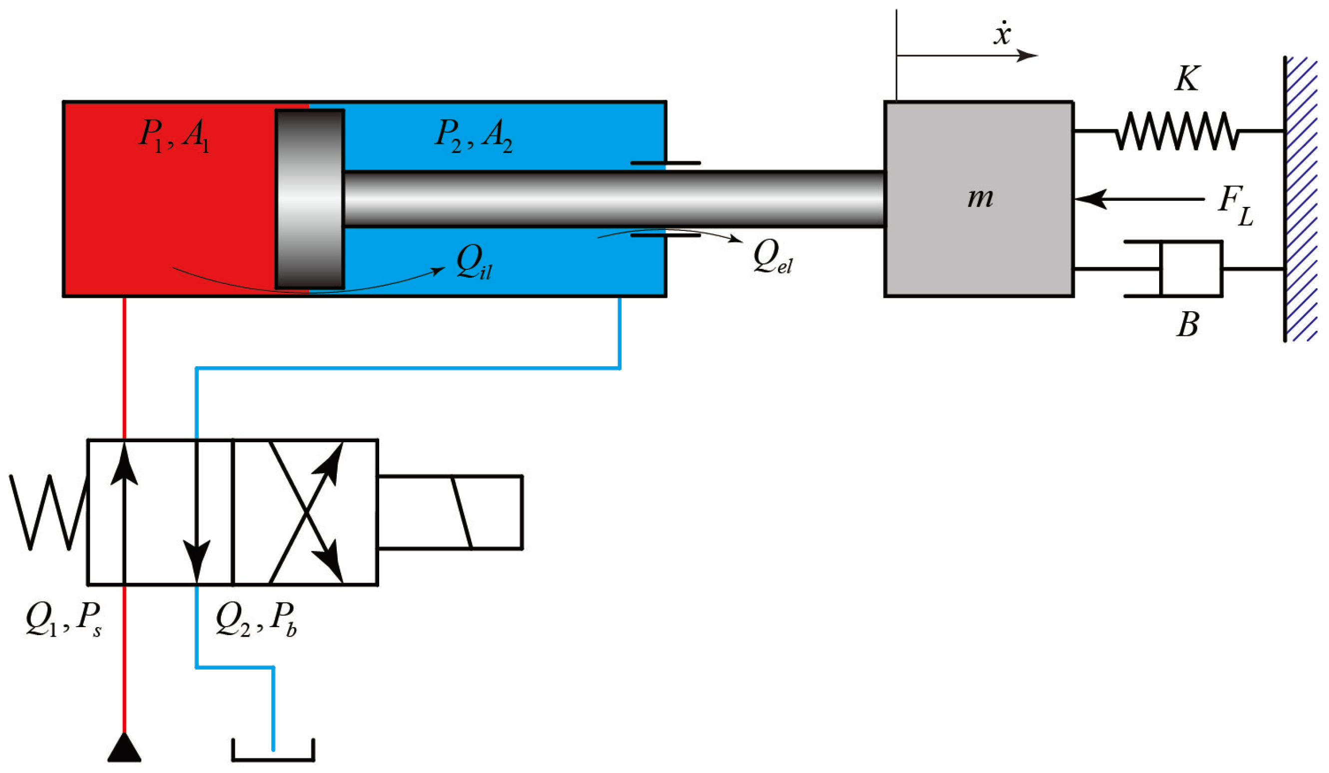
The schematic of the system is depicted in
Figure 2. The force of the cylinder is regulated by a fixed pressure source at the supply, and the direction of the piston motion is controlled by a directional control valve (DCV). For the purpose of facilitating analysis, the following assumptions are adopted:
- (1)
The temperature, viscosity, and bulk modulus of the working fluid remain constant.
- (2)
Leakage flows are characterized as laminar.
- (3)
The pressure within the working chambers of the cylinder is uniformly distributed.
Figure 2.
Schematic diagram of the system.
Figure 2.
Schematic diagram of the system.
Under these assumptions, we begin by examining the extension movement, with the DCV positioned to the left. The equation governing pressure buildup in the piston chamber of the cylinder can be expressed as follows:
The pressure buildup equation for the rod chamber of the cylinder can be expressed as follows:
The flow equation for the inlet port of the piston chamber in extension motion is as follows:
The flow equation for the outlet port of the rod chamber in extension motion is as follows:
For the retraction movement, the DCV is switched to the right position, and the pressure build-up equation for the piston chamber can be expressed as follows:
The pressure build-up equation for the rod chamber can be expressed as follows:
The flow equation for the inlet port of the piston chamber in retraction motion is as follows:
The flow equation for the outlet port of the rod chamber in retraction motion is as follows:
For both the extension and retraction cases, the motion equation of the piston is as follows:
The internal leakage can be expressed as follows:
The external leakage can be expressed as follows:
And the contact force can be expressed as follows:
Define the stats vector of the system as follows:
Define the input vector as follows:
Define the time-varying parameter vector as follows:
Based on the system model given in Equations (7)–(18), the state transition model of the system can be expressed as follows:
The system output can be expressed as follows:
To numerically solve the non-linear continuous-time state transition model, the 4th-order Runge–Kutta method is adopted in this study. The 4th-order Runge–Kutta method can be expressed as follows:
And the discrete output measurement is as follows:
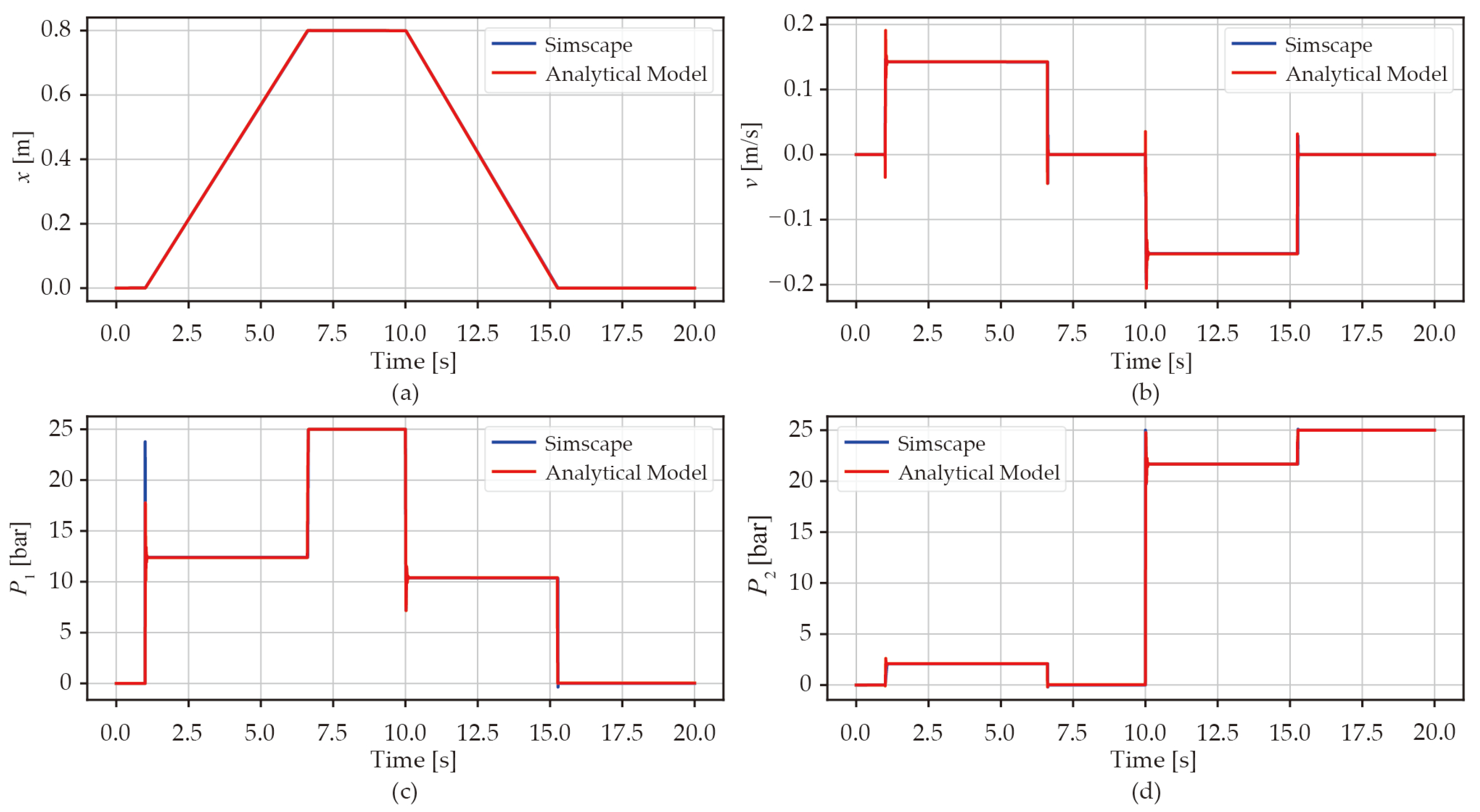
3.2. Verification of the Model
To validate the analytical model presented in the previous paragraphs, a Simulink
® SimScape model of the corresponding system was constructed. By employing the identical time-invariant parameters outlined in
Table 2, along with the designated input signals, a comparison was made between the output results of the analytical model and the SimScape model. This comparison is presented in
Figure 3. The evident agreement between the analytical model and the SimScape model serves to validate the efficacy of the analytical model. The small differences are given by the numerical integrator choice.
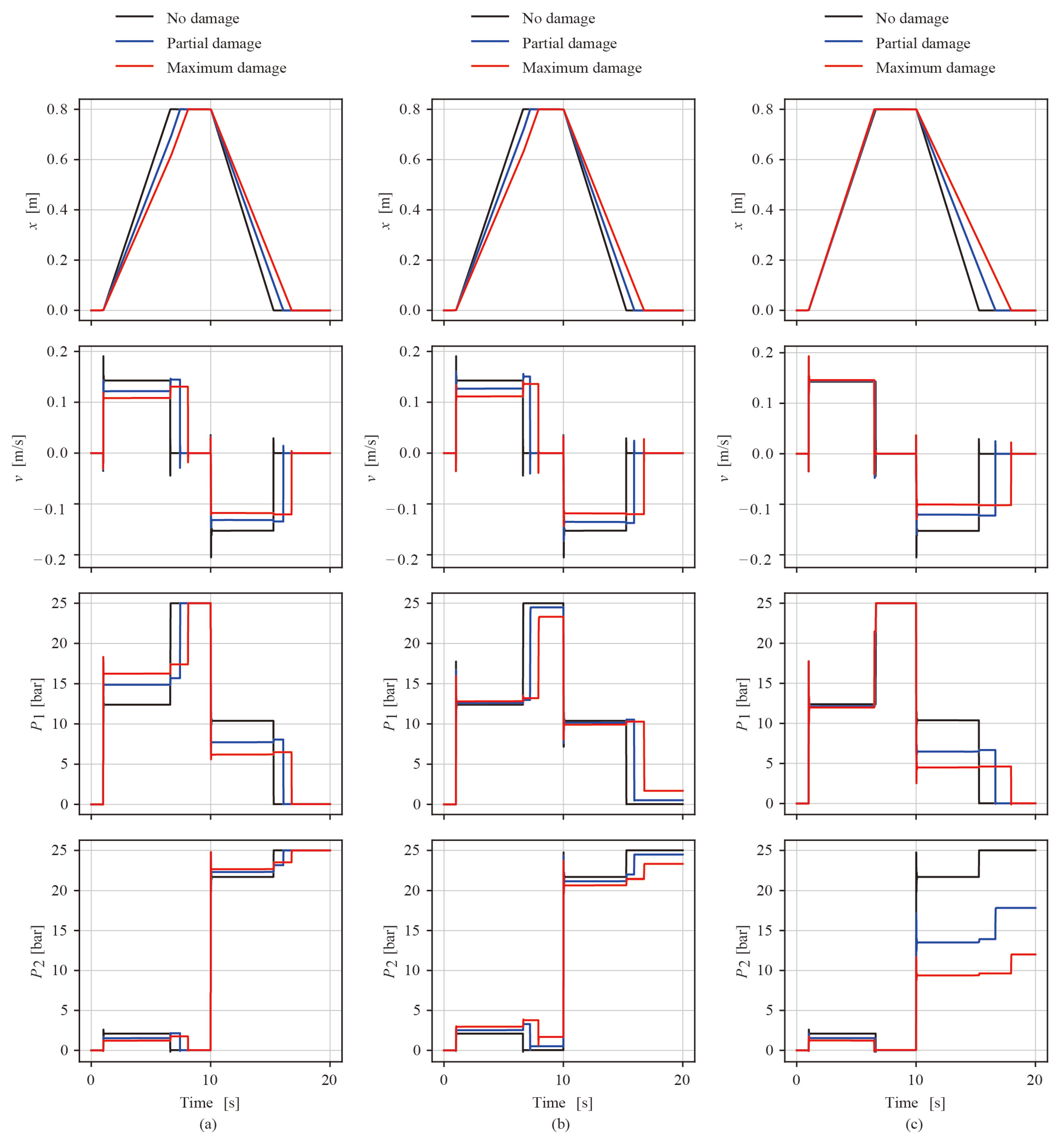
3.3. Impact of the Time-Varying Parameters
Upon confirming the efficacy of the analytical model, it becomes applicable for analyzing the impact of time-varying parameters on the system states. As illustrated in
Figure 4a, an increase in the viscous coefficient
B leads to a reduction in both extension and retraction speeds. Consequently, the time required to complete a full stroke increases. This is highly comprehensible since the viscous coefficient
B is directly associated with the friction force. During the extension stroke,
P1 functions as the working pressure, and
P2 acts as the back pressure. Conversely, in the retraction stroke,
P1 switches roles to become the back pressure, while
P2 becomes the working pressure. Throughout both strokes, the friction force consistently opposes the direction of motion. As a result, the impact of
B on
P1 and
P2 demonstrates a contrasting pattern. During the extension stroke, an increase in
B leads to a rise in
P1 and a decrease in
P2. Conversely, in the retraction stroke, an increase in
B causes
P1 to decrease and
P2 to increase. In magnitude, variations in
B have a notably substantial impact on
x,
v, and
P1, while the effect on
P2 is comparatively minor.
The internal leakage coefficient
Cil is directly connected to the rate of internal leakage flow via Equation (16). This influence of
Cil is depicted in
Figure 4b. The effect of
Cil on both
x and
v closely resembles that of
B. An increase in
Cil corresponds to a decrease in both extension and retraction speeds, consequently leading to an extended duration for extension/retraction. With an increase in
Cil, both
P1 and
P2 exhibit slight increments during the extension stroke, while they decrease in the retraction stroke. Notably, the influence of
Cil on
P2 is slightly more pronounced than on
P1. The variation in
Cil has a more prominent effect on
P1 and
P2 when the piston is at rest compared to when it is in motion.
The external leakage coefficient
Cel corresponds to the rate of external leakage flow, as shown in Equation (17). Referring to
Figure 4c, an increase in
Cel has a minor effect on the extension speed, but significantly reduces the retraction speed. This disparity in impact can be attributed to the occurrence of external leakage exclusively at the piston rod seal. Consequently, the influence on the pressure in the rod chamber (
P2) is notably greater than that on the pressure in the piston chamber (
P1).
It is evident that the time-varying parameters exert substantial influences on the system’s state variables, leading to diverse system performances. If the performance no longer aligns with the specified requirements, it can be inferred that a fault has occurred. With reference to the three time-varying parameters, three distinct fault modes can be identified for hydraulic cylinders: friction fault, internal leakage fault, and external leakage fault.
Note that various factors, including temperature, viscosity, bulk modulus, and the presence of contaminants within the working fluid, among others, can also significantly influence the performance of a hydraulic cylinder and potentially lead to malfunctions. It is important to recognize that these parameters are characteristics of the working fluid itself and not inherent properties of the cylinder. Consequently, in this study, we treat these fluid-related parameters as constant values over time.
Friction, internal leakage, and external leakage in a hydraulic system collectively impact both system functionality and the environment. Excessive friction within the system can lead to reduced efficiency, heat generation, component wear, and decreased precision, all of which can affect its overall performance. Internal and external leakage reduce efficiency through the loss of hydraulic fluid. Meanwhile, external leakage presents significant environmental concerns, as it can result in the release of hazardous hydraulic fluid into the surroundings, posing threats to ecosystems and human safety.
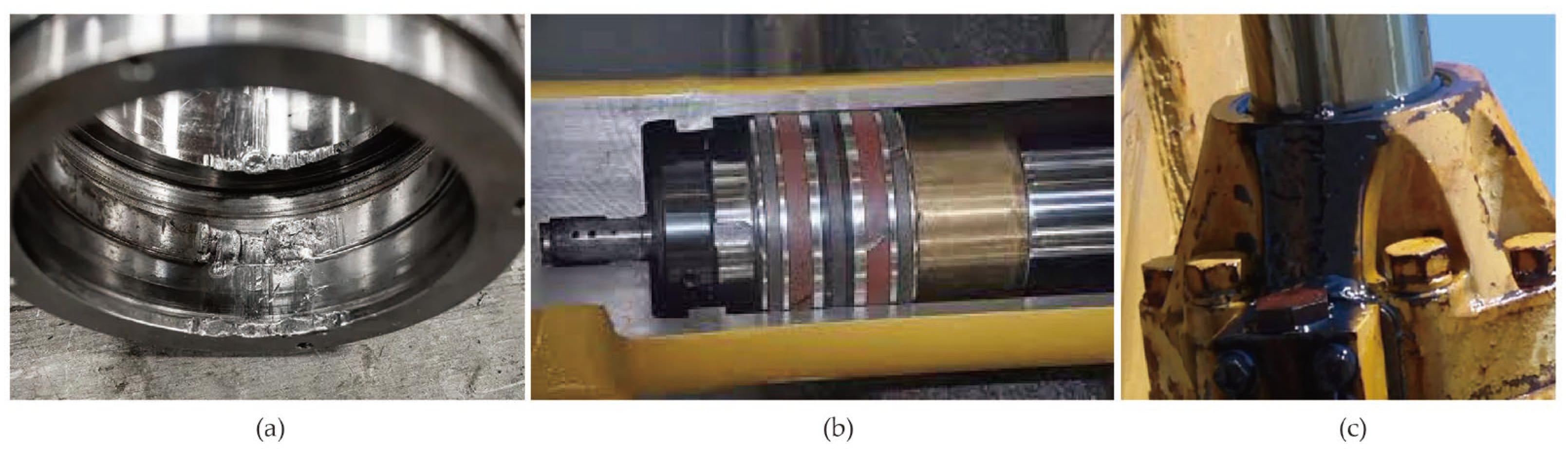
The most common causes of friction-related faults include, but are not limited to, worn seals or guides, the presence of contaminants, side-loading, and component damage. Within a hydraulic cylinder, seals, including piston and rod seals, can generate friction when they come into contact with the cylinder walls and moving components, such as the piston rod. If these seals become worn or damaged, they have the potential to increase friction levels. Particles or contaminants in the hydraulic fluid can infiltrate the space between the seals and the cylinder walls, leading to heightened friction. Additionally, improper alignment of the hydraulic cylinder or uneven distribution of the load can result in uneven pressure on the cylinder walls. In some extreme cases, this can cause the cylinder rod to bend, ultimately resulting in increased friction. Lastly, the wear and tear of components like piston rods and cylinder walls, as illustrated in
Figure 5a [
26], can also contribute to an increase in friction.
Both internal and external leakage can result from a variety of factors, including damaged or worn seals, contaminants, cylinder and rod damage, excessive pressure, and more. Among the primary contributors to both types of leakage are deteriorated or worn seals within the hydraulic cylinder. Seals can deteriorate over time due to factors like friction, pressure, contamination, and extreme temperatures. Physical damage to the hydraulic cylinder or rod, such as nicks, scratches, bends, or corrosion, can affect the rod seal and cause fluid to leak both internally and externally. Operating the hydraulic system at pressures exceeding its design limits can induce seal failure, contributing to both internal and external leakage. The phenomenon of hydraulic cylinder leakage is depicted in
Figure 5b,c [
27].
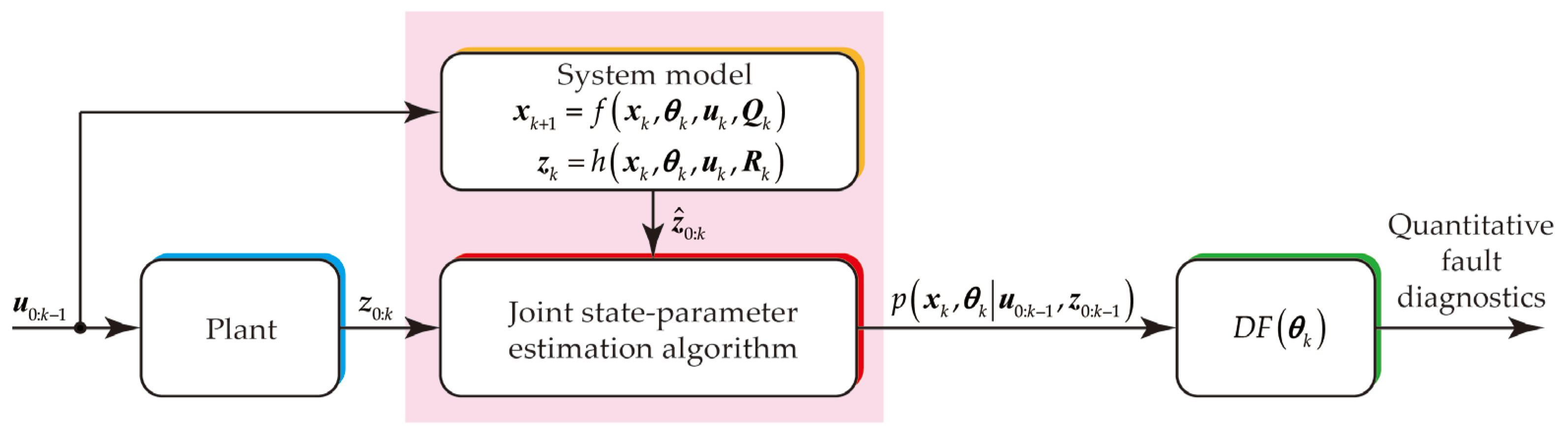
4. Joint State-Parameter Estimation
In this study, we utilize a particle filter to conduct joint state-parameter estimation. This choice is made because the hydraulic cylinder model exhibits non-linearity, and there is no evidence supporting the assumption of a Gaussian distribution of the state parameter. The particle filter method approximates the posterior distribution through Monte Carlo sampling. Specifically, a particle filter utilizes a set of independent random realizations, referred to as particles, which are directly sampled from the state space. These particles serve as representations of the posterior probability and are updated as new observations become available. The Bayesian formula is employed to appropriately position, weight, and recursively propagate the particles.
To realize joint state-parameter estimation, the state vector is augmented with the time-varying parameter vector as follows:
In this way, the state and time-varying parameters can be estimated simultaneously. Since the time-varying parameters for the hydraulic cylinder typically exhibit slow growth in practice, it is reasonable to assume that their time derivatives are zero in the state transition model.
In a particle filter, the augmented state distribution at time step
k is approximated by a set of weighted particles, as follows:
where the superscript
i is the particle index, subscript
k is the time step,
N denotes the number of particles,
is the augmented state particles, and
is the non-negative numerical factors named importance weights, which sum to one. Each particle
represents a possible realization of the augmented state. The importance weight
represents the relative importance of each of the
N particles.
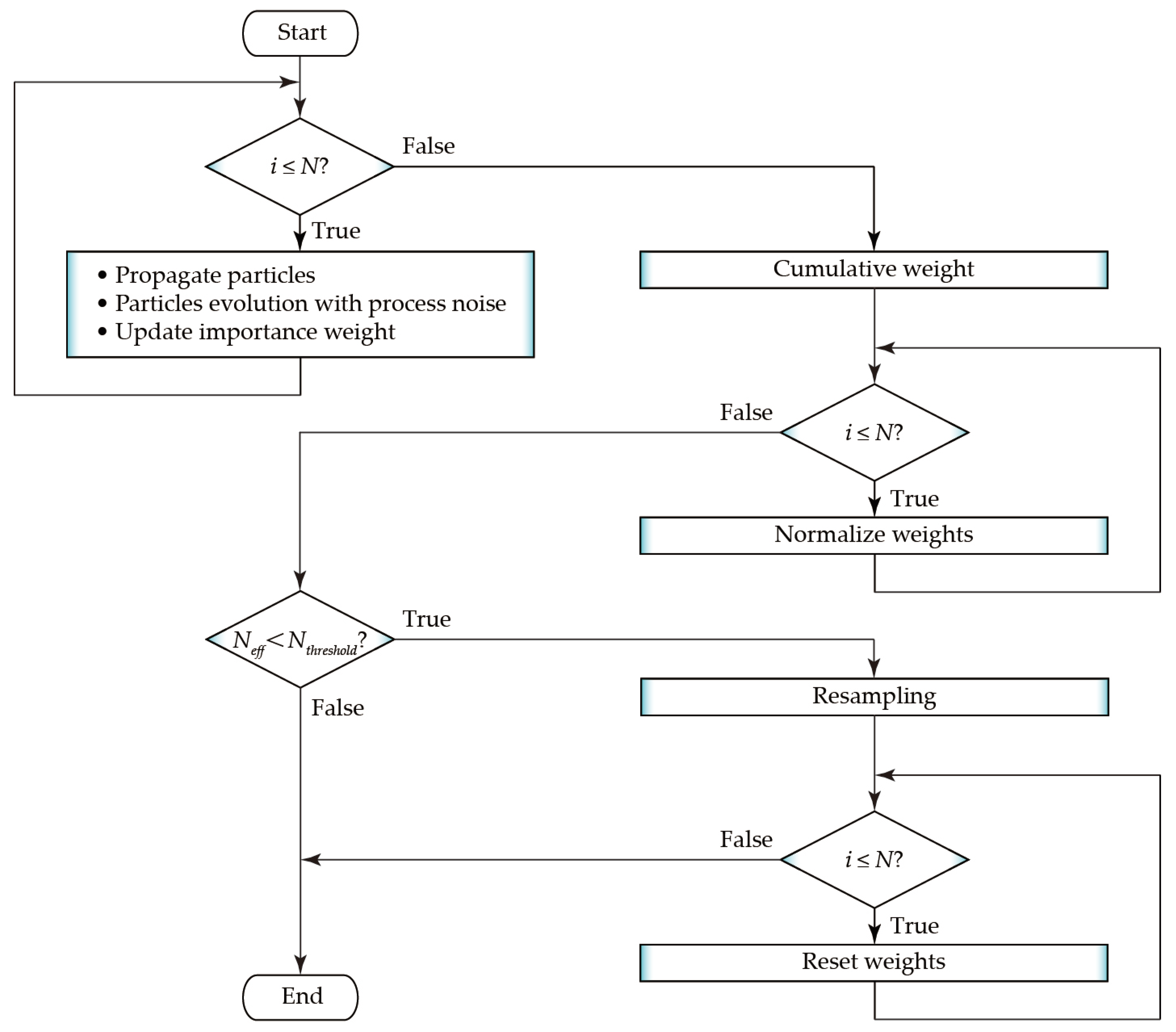
In this study, the sequential importance sampling with resampling (SISR) particle filter is utilized. The pseudocode for a single time step of the SISR particle filter is given in Algorithm 1, and the corresponding flow chart is depicted in
Figure 6. The algorithm takes in a set of weighted particles
that represents the previous belief of the augmented states, as well as inputs from control action
and measurement
. It then calculates and provides the updated state distribution
. Each particle is propagated forward to time step
k by using the state transition model
established in
Section 3.1. The propagated particles are then evolved by adding assumed Gaussian process noise. The importance weight is updated based on the measurement
. Specifically, the measurement model
is applied to the propagated particles to calculate the estimated output
, and the likelihood of their corresponding outputs is calculated using the assumed probability density function of the measurement noise, as shown in Equation (28).
| Algorithm 1: Sequential importance sampling with resampling particle filter |
| Input: , , |
| Output: |
| for i = 1 to N do |
| | # Propagate particles |
| | # Particles evolution with process noise |
| | # Update importance weight |
| end |
| # Cumulative weight |
| for i = 1 to N do |
| | # Normalize weights |
| end |
| if then # Resample if needed |
| | Resample N particles with replacement |
| | for i = 1 to N do |
| | | # Reset weights |
| | end |
| end |
where
nm is the number of the measurement, equal to 4 in our case, and
is the covariance matrix. The mean vector of this distribution is set to be equal to the estimated output
, and the covariance matrix equals the covariance of the measurement noise. We evaluate this distribution at the actual measurement
. Then, we multiply the resulting values together to obtain a single likelihood value for the particle. Once the weights are updated for each particle, a normalization step is performed. This normalization involves dividing each particle’s weight by the cumulative sum of all the weights, ensuring that they collectively add up to one.
A particle filter typically begins with initialized particles, all assigned equal weights. However, only a few particles may be positioned close to the true values of the augmented state. As the algorithm progresses, any particle not aligning with the measurements will receive an extremely low weight, while those particles in proximity to the true augmented state values will carry a significant weight. When the filter encounters this scenario, it becomes degenerate. Typically, this problem is resolved by using some form of particle resampling. To minimize computational expenses, particle degeneracy is evaluated by calculating the effective sample size, as represented in Equation (29):
Resampling is performed whenever the effective sample size falls below a threshold, Nthreshold. Following resampling, the particle weights are set to equal values of 1/N.
After updating the weights and particles using Algorithm 1, one can calculate the estimated augmented states at time step
k by simply summing the weighted values of the particles:
The confidence interval (CI) can be determined by calculating the nth percentile of the particles. For instance, the lower boundary of the 95% CI corresponds to the 2.5th percentile of the particles, whereas the upper boundary corresponds to the 97.5th percentile of the particles.
For a deeper explanation of the theoretical aspects of the particle filter, readers can refer to references [
28,
29].
5. Performance Evaluation and Analysis
To evaluate the performance of the proposed method, we designed four experiments, as outlined in
Table 3. Specifically, Exp. 1 serves as a baseline. In comparison to Exp. 1, Exp. 2 involves altering the true values of the parameters to assess the method’s performance when dealing with variations in parameter values while keeping the operating conditions the same. In contrast, Exp. 3 maintains the same parameter values as Exp. 1 but changes the operating conditions to evaluate the generalization ability of the proposed method under different operational scenarios. Exp. 4 is used to further test the robustness of the proposed method, where both the operating condition and parameter values are changed with respect to the first three experiments. Note that varying parameter values correspond to different degrees of fault severity.
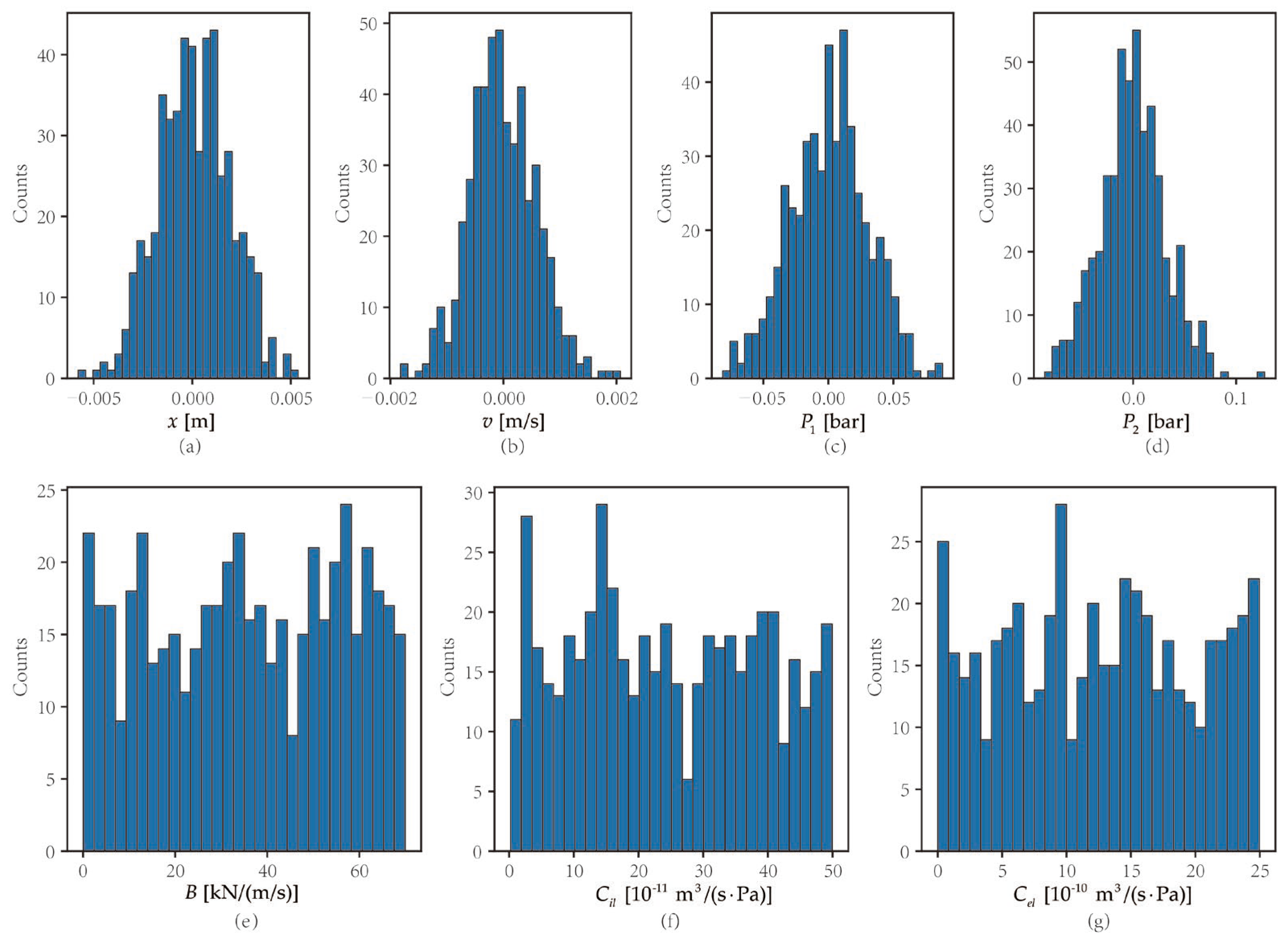
In all four experiments, the true values and measurements are obtained from the SimScape simulation, and the number of particles is consistently set at 500. The initialization of the particles in experiment 1 is depicted in
Figure 7. Specifically, since the states can be measured using sensors, we initialize the state particles using a Gaussian distribution based on the mean and standard deviation values given in
Table 4. Conversely, for the time-varying parameters, no additional information is available aside from their minimum and maximum values. Therefore, the time-varying parameter particles are initialized using a uniform distribution with the corresponding minimum and maximum values given in
Table 4. The same initialization method was employed for the other experiments.
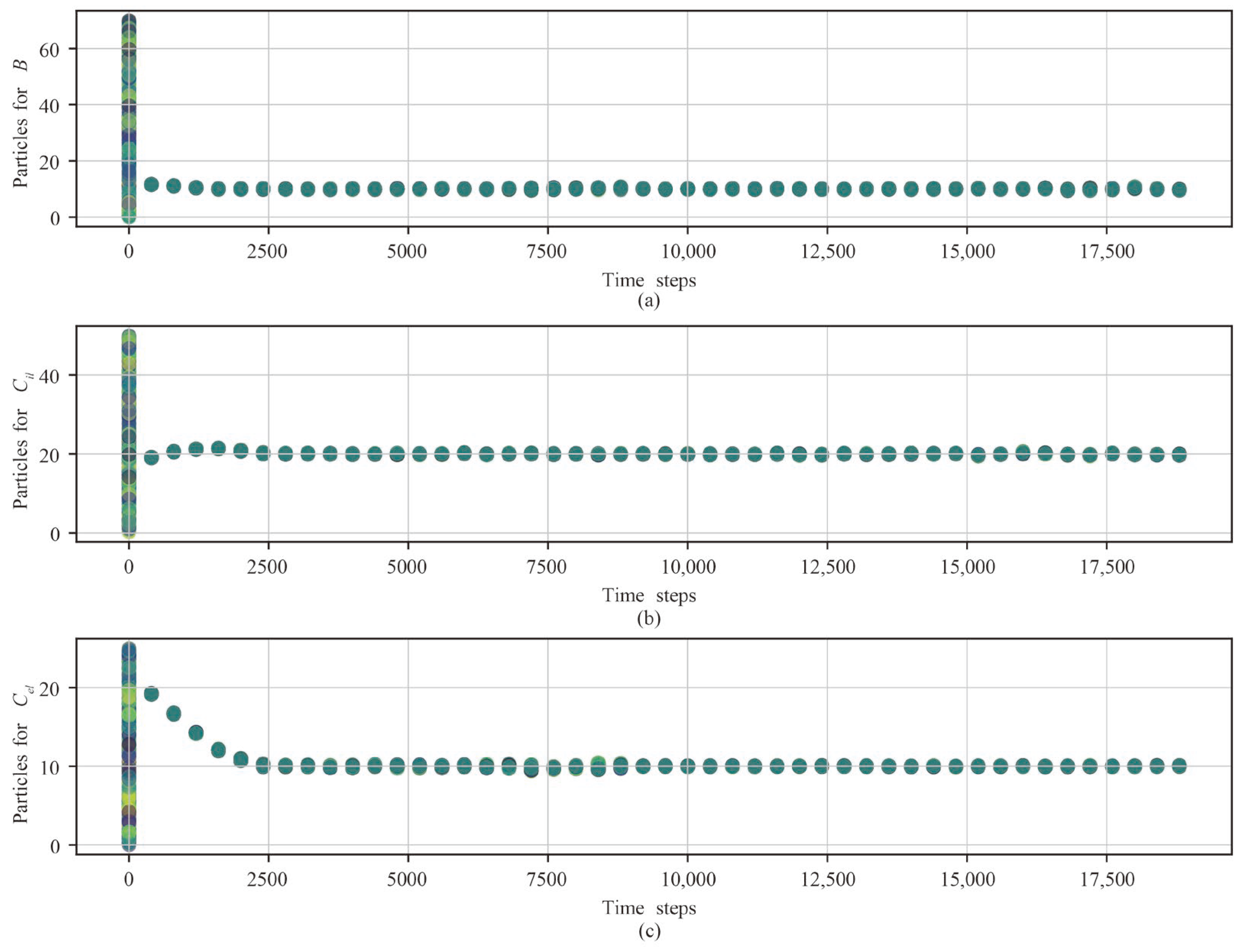
The evolution of the particles for the time-varying parameters of experiment 1 is depicted in
Figure 8 at intervals of 400 time steps. It is important to recognize that the dispersion of the particles reflects the level of uncertainty. At time step 0, the particles are uniformly distributed within the respective minimum and maximum values of the time-varying parameters, signifying the highest level of uncertainty. As the iterations progress, the particles concentrate together, indicating a significant reduction in uncertainty. Meanwhile,
Figure 8 serves as evidence of the particle filter algorithm’s convergence. One can observe different convergence rates among the parameters. Notably, the viscous coefficient
B converges most rapidly, whereas the external leakage coefficient
Cel converges more slowly, and the convergence speed of the internal leakage coefficient
Cil falls in between.
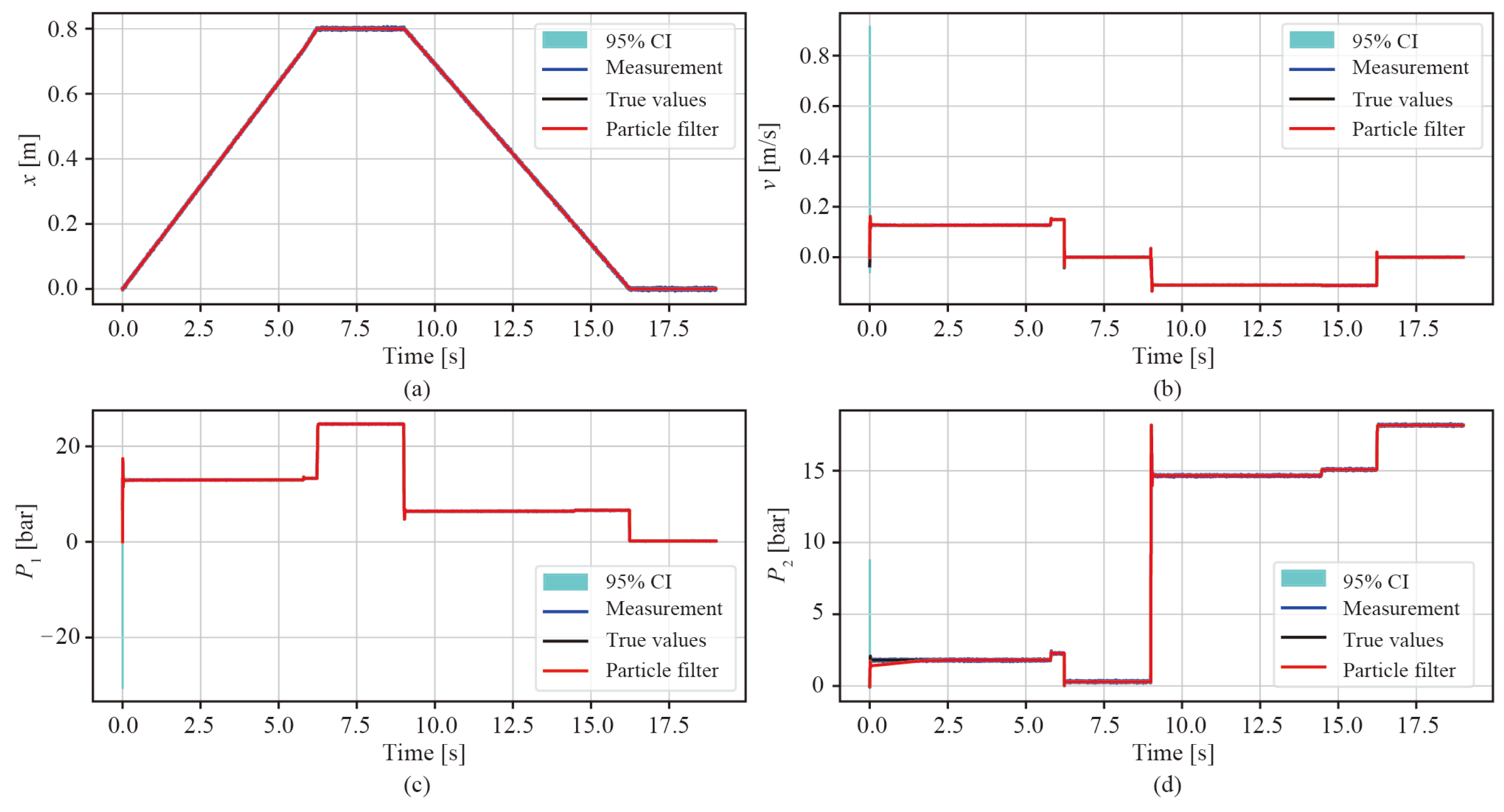
The state estimation results and their corresponding 95% confidence intervals (CIs) for Exp. 1 are depicted in
Figure 9. As evident from the observation, the particle filter state estimations demonstrate a high level of accuracy, closely matching the corresponding true values. Note that in
Figure 9, with the exception of the initial time step, the 95% CIs are conspicuously narrow and closely aligned with the estimations, indicating a minimal level of uncertainty associated with the estimations. This result can also be supported by
Figure 8, where it is evident that the particles representing the possible parameter values cluster closely together. It can also be observed that the state estimation values exhibit smaller variations in comparison to the measurement values, resulting in more accurate state values than those provided by the sensors.
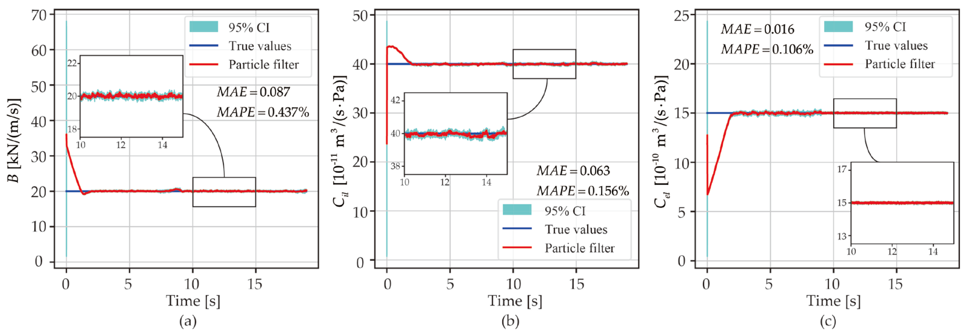
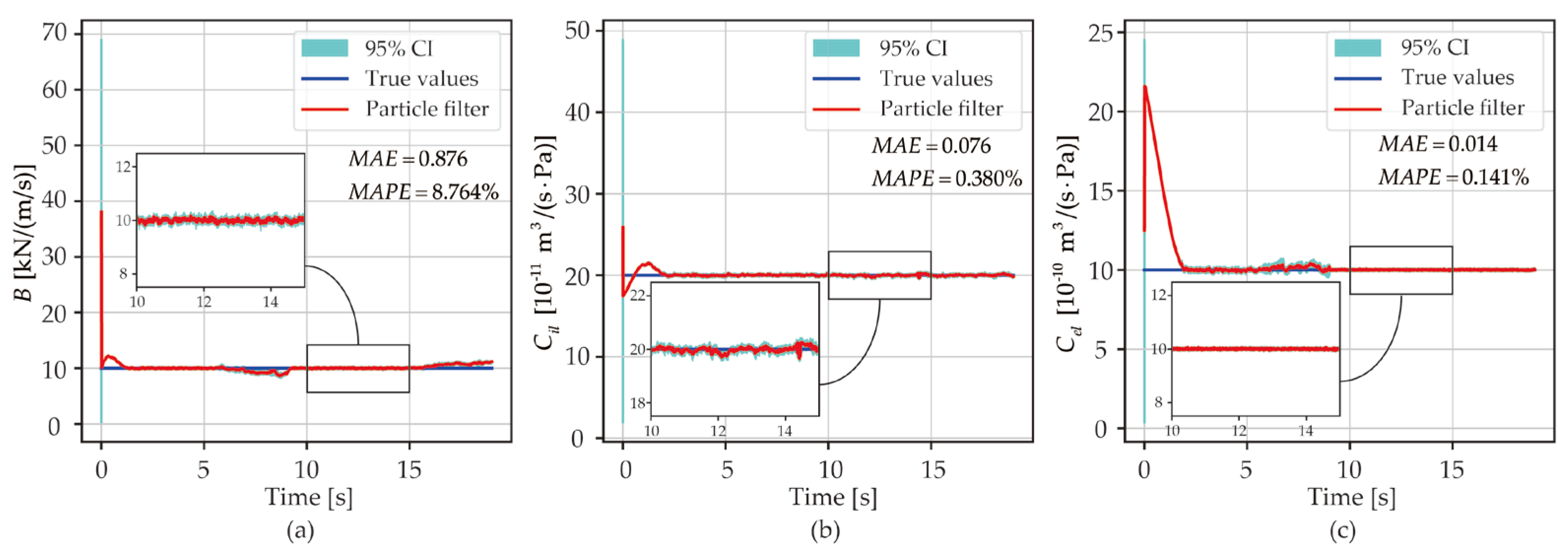
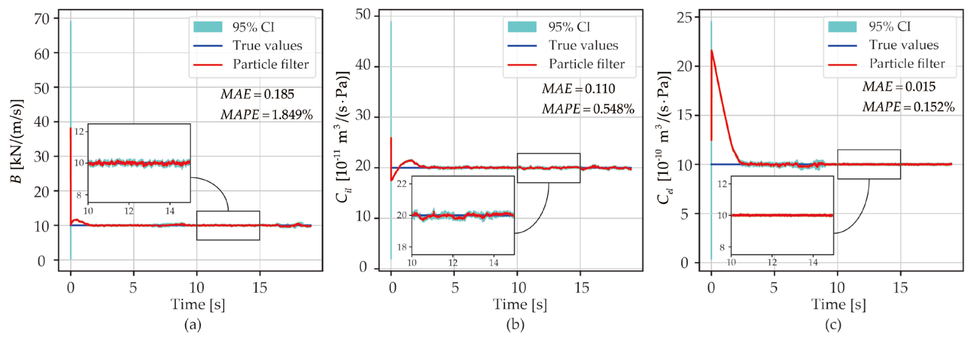
Compared to state estimation, our primary focus is on the estimation of time-varying parameters. This emphasis is due to the fact that the time-varying parameter values are directly related to the degree of health of the cylinder. The time-varying parameter estimation results and the corresponding 95% CIs for Exp. 1 are illustrated in
Figure 10. To quantitatively assess the accuracy of the estimations, we employ the performance metrics known as the mean absolute error (MAE) and mean absolute percentage error (MAPE), as respectively defined in Equations (31) and (32). In these equations,
n represents the number of data points,
y stands for the true value, and
denotes the estimated value. These values are also depicted in
Figure 10 for reference. After convergence, the particle filter estimation results closely match the true values, offering a reliable estimate of the time-varying parameter values under the operating conditions of Exp. 1. The 95% CIs are notably tight, ensuring high-confidence estimations.
The time-varying parameter estimation results for Exps. 2 and 3 are illustrated in
Figure 11 and
Figure 12, respectively. The results of Exp. 4 are demonstrated in
Table 5. It is clear that the particle filter is capable of providing accurate parameter estimations even when faced with varied parameter values and different operating conditions. By employing parameter value estimations, Equation (5) can be applied to determine the degree of the fault, thus enabling a quantitative fault diagnostic of the hydraulic cylinder.


