Application of Multiple Deep Neural Networks to Multi-Solution Synthesis of Linkage Mechanisms

Abstract

This paper studies the problem of linkage-bar synthesis by means of multiple deep neural networks (DNNs), which requires the inverse solution of linkage parameters based on a desired trajectory curve. This problem is highly complex due to the fact that the solution space is nonlinear and may contain multiple solutions, while a good quality of learning cannot be obtained by a single neural network approach. Therefore, this paper proposes employing Fourier descriptors to represent trajectory curves in a systematic and normalized form, developing a multi-solution distribution evaluation by random restart local searches (MDE-RRLS) to examine a better solution-space partitioning scheme, utilizing multiple DNNs to learn subspace regions separately, and creating a multi-facet query (MFQuery) to cooperatively predict multiple solutions. The experiments demonstrate that the proposed approach can obtain better or at least competitive outcomes compared to previous work in the literature. Furthermore, to verify the effectiveness and applicability, this paper investigates the design problem of an industrial six-linkage-bar ladle mechanism used in a die-casting system, and the proposed method can obtain several superior design solutions and offer alternatives in a short period of time when faced with redesign requirements.

1. Introduction

The linkage-bar synthesis problem is an inverse problem [1], which requires designing the linkage mechanism based on the expected kinematic characteristics and the inverse solution for each linkage parameter; however, the relationship between the shape of the coupling curves and the parameters of the linkage mechanism is highly nonlinear; furthermore, this type of inverse problem presents a high degree of complexity as it may have no solution, a single solution, or multiple solutions depending on the specific conditions [2].

Numerous prior studies have investigated linkage synthesis problems, with prevailing solution methods encompassing geometric derivation, algebraic analysis, and numerical methods [3]. The first two can comprehend mechanism parameters through the mathematical derivation process; however, such methods have limitations due to the number of precise points. When the number of points to be synthesized exceeds the number of mechanism parameters, it is typically impossible to find exact paths through all the points. Consequently, numerical methods are used to obtain an approximate solution, which is the main solution method when dealing with a large number of points.

Numerical methods rely on the analysis of linkage-bar motion to establish an approximate mathematical model. Through the designed objective function of the coupling error, various numerical algorithms are employed to solve for the optimal solution, such as gradient methods [4]. Nevertheless, such methods have their limitations, including the difficulty of selecting an appropriate initial value and algorithms to jump out the local solution, making it arduous to get the global solution [5]. Therefore, researchers have explored the global solution scheme using heuristics methods, including genetic algorithm (GA) [6,7], particle swarm optimization (PSO) [8], and differential evolution (DE) [9].

Heuristic methods are used for exploration and searching for equivalent models in the solution space to provide a set of inverse solutions to choose from. These methods do not directly solve the inverse problem, but rather, employ searching or sampling. They use only the forward model to compute diverse sample values. For these global methods, the crucial factor is the number of forward solutions [10] (i.e., the number of evaluation function calls) needed to compute when sampling an uncertain region. Despite the presence of uncertainty [11], the problem remains solvable, and typically, there is no requirement to introduce a priori knowledge in the primary schema. As a result, heuristic methods provide a more generalized approach to solving the inverse problem. However, since iterative correction of the search direction in loops is usually used to approximate the optimal solution and requires a large amount computation, heuristic methods are difficult to provide real-time or fast synthesis results.

Furthermore, in the design of linkage bars, it is common to borrow similar designs from the past to aid in finding a solution; in the literature, the atlas database method involves creating a database of linkage curves beforehand, and then obtaining the closest design solution by using the table lookup method [12]. However, this approach necessitates a suitable curve representation, an appropriate database size, and an efficient process for searching the linkage-bar database. Additionally, obtaining a new solution between the pre-existing cases requires a proper interpolation method, however, such a solution is often challenging to acquire, resulting in limitations.

Researchers have attempted to overcome the limitations of the numerical and heuristic methods by adopting the artificial neural network (ANN) method. Using pre-learning ANN models, they can efficiently provide rapid solutions for synthesis. Compared to the atlas dataset method, ANN methods offer robust properties that allow for predicting new solutions without pre-existing a linkage database [13]. Therefore, this paper investigates the potential of utilizing neural networks as a means for dimension synthesis and evaluates the advantages over existing approaches reported in the literature.

On the other hand, even minor variations in linkage-bar configurations or parameters may result in trajectory curves of various shapes, sizes, or orientations due to nonlinear factors, and thus many feasible designs may be missed when synthesizing. Therefore, prior research has worked to systematize and normalize the representation for closed trajectory curves [14,15]. This is done to reduce the high complexity and dimensionality in the neural coupling problems that arises from scaling, rotation, and displacement of trajectory output from linkage-bars. Hoskins & Kramer [16] attempted to represent the curves in a power spectrum manner and learn the four-linkage-bar synthesis problem with radial basis function ANN; however, their study fixes multiple linkage parameters directly and explores the solution for only a small region of variation of two link parameters, which is limited in applicability. Yannou & Vasiliu [17] showed the shape of the path by the Fourier coefficients of the harmonic analysis and used the Stuttgart neural network simulator (SNNS) for the function approximation of linkages, their study emphasized that ANNs provide fast access to coupling solutions and are suitable to be built into interactive tools. In addition, ANNs that have learned tens of thousands of cases require very little storage as compared to the atlas method. However, the discussion on linkage design acknowledges the existence of a one-to-many mapping problem, but lacks suggestions for further improvement. Instead, the focus is on recommending appropriate selection of dimensional parameters and their respective value intervals. Galán-Marín et al. [13] used a wavelet as a curve representation and focused on the coupling problem of the Crank-Rocker mechanism, but did not validate the applicability of other types, such as the Crank-Crank mechanism. Khan et al. [18] used Fourier descriptor (FD) of cumulative angular deviation of the curve, and also explored only the coupling problem of the Crank-Rocker mechanism and used multilayer feed-forward neural network (MLFFNN) to learn the coupling problem; however, some coupling results were significantly worse for the generalized curves in the cases they discussed. Li & Chen [19] explore the parametrization-invariant method to eliminate the influence of parametrization under FD, normalization with the arc length approach, and then learning by MLFFNN. However, according to the original paper, the quality of the ANN solution can be further improved. Table 1 collates information from existing literature about neural-network-based linkage synthesis and indicates the curve descriptor, neural network model, and applicable mechanism types used in each study for reference.

As previously discussed, the ANN method may provide a fast solution, but it struggles to solve the linkage-bar synthesis problem well when faced with multiple solutions [19]. Additionally, in cases where there are instances with identical inputs but different outputs within the dataset, the training quality and convergence of the ANN are significantly reduced. This phenomenon can be confirmed by examining specific cases outlined in the subsequent sections. However, although solving the multiple solution problem presents challenges, it can provide more flexibility in applications [20]. For example, multiple sets of inverse solutions can encourage the decision-maker to consider factors that are less easily modeled (e.g., difficult machining) to select the most appropriate solution. Therefore, unlike the previous research in which a single solution scheme was mainly considered, this paper employs multiple deep neural networks (DNNs) to learn the relationship between the Fourier coefficients and linkage-bars. This enables the development of a fast solution scheme for linkage synthesis and allows individual DNNs to learn the partitioned sub-solution spaces to cooperatively generate multiple sets of candidate solutions. Although some recent studies use generative artificial intelligence (Generative AI), such as Auto Encoder [21], to explore multiple solutions to linkage synthesis, their primary focus is on generating diverse solutions. Coupling refinement is usually a secondary consideration, and their direction is still distinct from the cooperative solutions towards refinement proposed in this paper.

Since the proposed approach involves the construction of multiple DNNs, arranging the learning datasets appropriately to maximize the overall learning quality has become a critical issue. To effectively tune the learning performance of multiple DNNs, this paper first proposes a multi-solution distribution evaluation using the random restart local searches (MDE-RRLS) method. This sampling method examines the better sub-solution space partitioning scheme when training multiple DNNs. Additionally, a multi-facet query (MFQuery) is also proposed to form additional coupling targets by utilizing vertical and horizontal projections on the trajectory curves. This expands the solution coverage of the dataset. Subsequently, a voting method or threshold filtering process can be used to gather one or multiple candidate solutions.

In addition, to assess the scalability of the proposed solution, the paper investigates the design issues of a six-linkage-bar ladle used in metal-mold die-casting machine system [22]. Unlike the aforementioned four-linkage-bar case, this ladle mechanism does not require closed-curve motion and cannot be directly converted by the Fourier transform; this paper proposes expanding the motion curve into a closure-curve motion through geometric projection and training multiple DNNs to solve the design problem.

To summarize, the contributions of this study mainly come from: (1) The multi-DNNs strategy proposed in this study can obtain superior solution quality while also providing multiple candidate solutions, in contrast to prior single-solution schemes; (2) This study proposes a comprehensive multi-DNNs learning and prediction process, encompassing the MDE-RRLS, the MFQuery and the voting methods; (3) This study extends and validates the synthesis scheme with non-closed trajectories, providing a fast and feasible solution for the redesign needs due to practical variations in the design of an industrial six-linkage-bar mechanism.

Table 1. List of the publications in linkage synthesis based on neural networks.

References	Year	Mechanism	Curve Descriptor	NN Model	Additional Features (Selected Portions Only)
Hoskins & Kramer [16]	1993	Crank-Rocker	Power spectrum	Radial basis NN	Hybridizing a gradient-based numerical method
Yannou & Vasiliu [17]	2001	Crank-Rocker	Fourier series	MLFFNN	Developing an integrated predesign platform RealisMe
Xie & Chen [23]	2007	Crank-Rocker	Fourier series	MLFFNN	Extending FD to the image space of kinematic mapping
Erkaya & Uzmay [24]	2009	Slider-Crank	Cartesian positions	MLFFNN	Modelling joint clearance as a massless link
Galán-Marín et al. [13]	2009	Crank-Rocker	Wavelet	MLFFNN	Sampling precise points at a non-constant time interval
Khan et al. [18]	2015	Crank-Rocker	Fourier series	MLFFNN	Hybridizing a local optimization procedure
Ahmadi et al. [25]	2016	General four-bar	Cartesian positions	GMDH-type NNs	Integrating game theory and multi-objective optimization
Li & Chen [19]	2017	General four-bar	Fourier series	MLFFNN	Proposing arc length normalization
Deshpande & Purwar [21]	2018	General four-bar	Signature method	Auto-Encoder	Integrating machine learning and computational kinematics for defect-free and part-to-whole synthesis
Mo et al. [26]	2019	Crank-Rocker	Fourier series	MLFFNN	Obtaining a high precision linkager mechanism
Yim et al. [27]	2021	General four-bar	Fourier series	Deep MLFFNN	Determining mechanism topology and end-effector location simultaneously based on big data
Kapsalyamov et al. [28]	2022	Six-linkage-bar	Cartesian positions	Deep MLFFNN	Integrating computational kinematics and machine learning to syntherize two joint trajectories (ankle and knee)
Yim et al. [29]	2023	Spatial linkage	Fourier series	Deep MLFFNN	Making the NN handle multi-class classification to improve the previous planar linkage synthesis approach

Table 1. List of the publications in linkage synthesis based on neural networks.

References	Year	Mechanism	Curve Descriptor	NN Model	Additional Features (Selected Portions Only)
Hoskins & Kramer [16]	1993	Crank-Rocker	Power spectrum	Radial basis NN	Hybridizing a gradient-based numerical method
Yannou & Vasiliu [17]	2001	Crank-Rocker	Fourier series	MLFFNN	Developing an integrated predesign platform RealisMe
Xie & Chen [23]	2007	Crank-Rocker	Fourier series	MLFFNN	Extending FD to the image space of kinematic mapping
Erkaya & Uzmay [24]	2009	Slider-Crank	Cartesian positions	MLFFNN	Modelling joint clearance as a massless link
Galán-Marín et al. [13]	2009	Crank-Rocker	Wavelet	MLFFNN	Sampling precise points at a non-constant time interval
Khan et al. [18]	2015	Crank-Rocker	Fourier series	MLFFNN	Hybridizing a local optimization procedure
Ahmadi et al. [25]	2016	General four-bar	Cartesian positions	GMDH-type NNs	Integrating game theory and multi-objective optimization
Li & Chen [19]	2017	General four-bar	Fourier series	MLFFNN	Proposing arc length normalization
Deshpande & Purwar [21]	2018	General four-bar	Signature method	Auto-Encoder	Integrating machine learning and computational kinematics for defect-free and part-to-whole synthesis
Mo et al. [26]	2019	Crank-Rocker	Fourier series	MLFFNN	Obtaining a high precision linkager mechanism
Yim et al. [27]	2021	General four-bar	Fourier series	Deep MLFFNN	Determining mechanism topology and end-effector location simultaneously based on big data
Kapsalyamov et al. [28]	2022	Six-linkage-bar	Cartesian positions	Deep MLFFNN	Integrating computational kinematics and machine learning to syntherize two joint trajectories (ankle and knee)
Yim et al. [29]	2023	Spatial linkage	Fourier series	Deep MLFFNN	Making the NN handle multi-class classification to improve the previous planar linkage synthesis approach

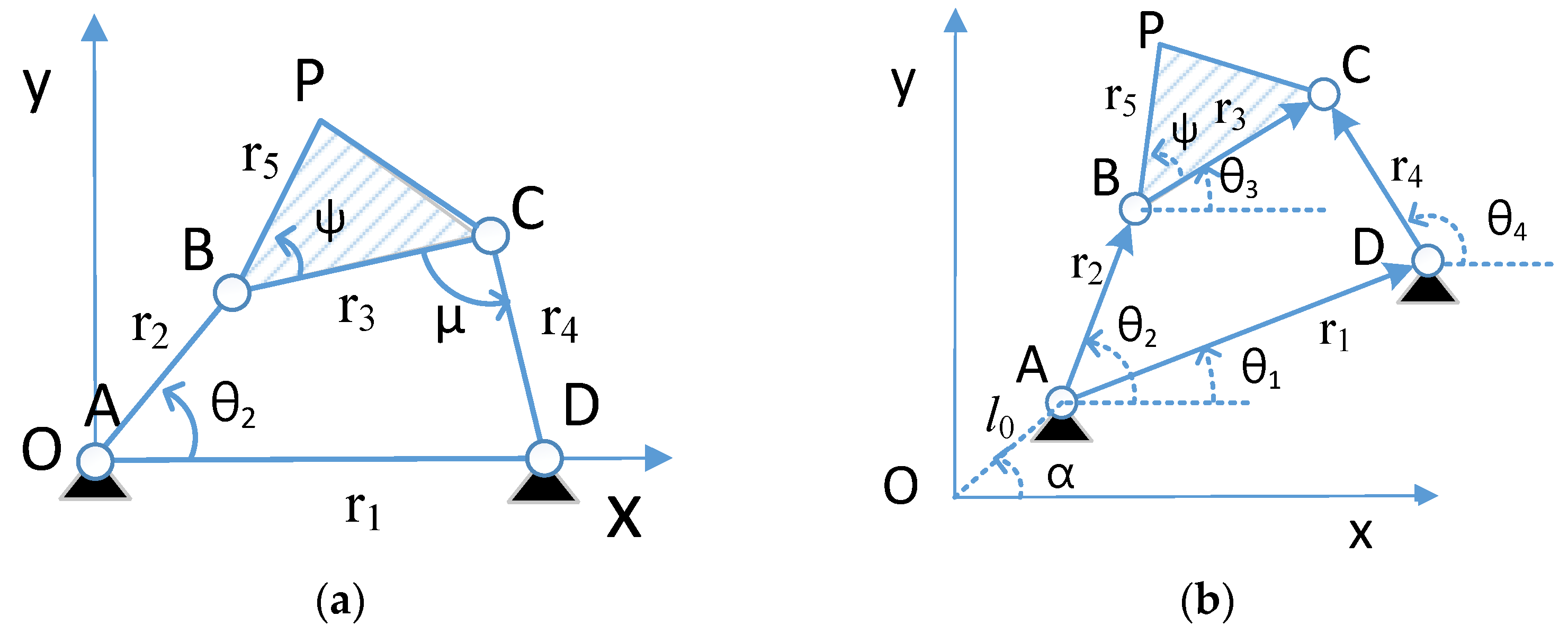
2. Problem Definition and Formulation

For a rigid body driven by a linkage-bar mechanism, when given a number of precise points to pass through, the goal of the synthesis design is to solve the linkage parameters inversely, in order to produce a desired trajectory curve that passes through a given set of precise points as accurately as possible [30]. When coupling a closed curve, one can apply a Fourier descriptor to obtain curve features and introduce a systematic normalization method to assist in the linkage-bar coupling procedure [31].

2.1. Fourier Descriptor Formulation

To analyze the periodic movement of a planar four-linkage-bar mechanism, the coordinate system shown in Figure 1a can be used. The framework uses O as the coordinate origin, coincides point A with origin O, and aligns the AD link with the x axis. Under the condition that $r_2$ can rotate a full 360 degrees, it is identified as a Crank link, in which the P-point will form a closed curve as it changes with time. The four linkage-bar mechanism is typically driven by the input angle ${\theta }_2$. To obtain the position of P at a certain point in time, it is necessary to combine the value of ${\theta }_2$ with the kinematic analysis of the lengths of the link-bars. This deduction can be achieved through the vector-loop method. Assuming that $\mathit{r}$ represents the vector of the link-bar r, the corresponding closure conditions are formulated as follows:

$${\mathit{r}}_1={\mathit{r}}_2+{\mathit{r}}_3-{\mathit{r}}_4,$$

(1)

Next, the component equations are used to derive:

$$r_{1}cos{\theta }_1=r_{2}cos{\theta }_2+r_{3}cos{\theta }_3-r_{4}cos{\theta }_4,$$

(2)

$$\mathrm{a}\mathrm{n}\mathrm{d} r_{1}sin{\theta }_1=r_{2}sin{\theta }_2+r_{3}sin{\theta }_3-r_{4}sin{\theta }_4.$$

(3)

By collapsing the above equations and analyzing the geometric relation of P and BC based on the parameters $r_5$ and $\phi$, the position of P can be expressed as a relation of $\left[r_1,r_2,r_3,r_4,\phi ,r_5\right]$ and ${\theta }_2$; the detailed derivation process can be referred to [32].

If $r_P\left(\mathrm{t}\right)$ represents the trajectory curve function of P during the motion, $r_P\left(\mathrm{t}\right)$ is a periodic function, and the period $\mathrm{T}=2\mathsf{\pi }$, $r_P(\mathrm{t}+\mathrm{T})=r_P\left(\mathrm{t}\right)$. The function can be represented by a complex function $r_P\left(\mathrm{t}\right)=x\left(\mathrm{t}\right)+iy\left(\mathrm{t}\right)$. When ${\theta }_2$ is moving at a constant speed $\mathsf{\omega }$, based on previous studies [14,33], ${\mathit{r}}_P$ can be expanded to a Fourier series in complex form:

$$r_P\left(\mathrm{t}\right)=x\left(\mathrm{t}\right)+iy\left(\mathrm{t}\right)={\sum }_{n=-\infty }^{\infty }{c}_n{e}^{in\omega t},$$

(4)

where $c_n$ is the n-th term of Fourier coefficients of the trajectory curve. In the Fourier descriptor, each item can be regarded as a circle whose radius is the magnitude of the coefficient, and these items are iterated to form the desired curve.

Since the process of synthesis typically involves passing through a finite number of precise points, using a Fourier descriptor to represent the curve requires that only a finite number of terms to be chosen to meet the necessary level of precision [17]. As a result, the precise points can serve as sampling points in this synthesis problem, with the corresponding coefficients obtained through application of the Fourier transform. If the number of retained terms is $2d+1$, this can be expressed as the following equation:

$$r_P\left(\mathrm{t}\right)\cong {\sum }_{n=-d}^d{c}_n{e}^{in\omega t}.$$

(5)

In practice, $d$ only needs to be a small number for the approximation error to be reduced to what is actually required [1].

On the other hand, a more generalized four-linkage-bar diagram can be represented in Figure 1b. From the diagram, the whole mechanism ABCDP is equivalent to a rotation of ${\theta }_1$ about the x-axis, and an offset of $l_0{e}^{i\alpha }$ with respect to the origin O. In this case, the coordinate transformed ${\mathit{r}}_P^{\prime }$ of ${\mathit{r}}_P$ is as follows:

$${\mathit{r}}_P^{\prime }=l_0{e}^{i\alpha }+{\mathit{r}}_P{e}^{i{\theta }_1}.$$

(6)

The transformed trajectory curve can be expanded as:

$$r_P^{\prime }\left(\mathrm{t}\right)\cong l_0{e}^{i\alpha }+{\sum }_{n=-d}^d{c}_n{e}^{in\omega t}·e^{i{\theta }_1}=l_0{e}^{i\alpha }+{\sum }_{n=-d}^d{c}_n{e}^{i({\theta }_1+n\omega t)}.$$

(7)

2.2. Fourier Coefficient Normalizing and Learning

To couple closed curves, normalization can reduce the dimensions that need to be synthesized. For example, shapes of curves produced by the same linkage-bar configuration with different origin coordinates can be normalized to the same shape. The normalization operations used in this paper include: (1) Normalization of the center point: setting the $c_0$ coefficient to 0, the center point is normalized to the origin (0,0); (2) Normalization of the orientation: rotating the curve to zero the phase angle of the $c_{-1}$ coefficient, it tends to align the orientation with the X-axis (horizontally); (3) Normalization of the curve size: dividing the amplitude of the coefficient $c_{-1}$ to all coefficients; and (4) Normalization of the length of the ground-link: setting $r_1$ as the base ($r_1$ = 1).

Indeed, in operations (2) and (3), they are not limited to the selection of the $c_{-1}$ term, and in the practical tests, the selection of either $c_1$ or $c_{-1}$ is very close to the effect. Based on the normalization rule, $r_P\left(\mathrm{t}\right)$ and $r_P^{\prime }\left(\mathrm{t}\right)$ are normalized to ${\overline{\mathrm{r}}}_P^{\prime }\left(\mathrm{t}\right)$ and ${\overline{\mathrm{r}}}_P^{}\left(\mathrm{t}\right)$, respectively, and their equations can be derived as follows:

$${\overline{\mathrm{r}}}_P^{\prime }\left(\mathrm{t}\right)\cong \frac{1}{c_{-1}{e}^{i({\theta }_1-\omega t)}}{\sum }_{n=-d, n\ne 0}^d{c}_n{e}^{i({\theta }_1+n\omega t)}$$

(8)

$$=\frac{1}{c_{-1}{e}^{i(-\omega t)}}{\sum }_{n=-d, n\ne 0}^d{c}_n{e}^{i({\theta }_1+n\omega t)}\cdot e^{-i{\theta }_1}$$

$$=\frac{1}{c_{-1}{e}^{i(-\omega t)}}{\sum }_{n=-d, n\ne 0}^d{c}_n{e}^{in\omega t}$$

$$={\overline{\mathrm{r}}}_P^{}\left(\mathrm{t}\right).$$

From the derivation, ${\overline{\mathrm{r}}}_P^{\prime }\left(\mathrm{t}\right)$ is equivalent to ${\overline{\mathrm{r}}}_P^{}\left(\mathrm{t}\right)$; therefore, the normalization eliminates the impact of the extra displacement and rotation of the mechanism. As a result, the simplified coordinate system as shown in Figure 1a is suitable for the normalized synthesis problem. Figure 2 shows an example of a trajectory curve obtained using the aforementioned normalization operations.

As shown in Figure 3, in the Fourier descriptor, the dimension synthesis problem is equivalent to the problem that synthesizing Fourier coefficients with the linkage-bar parameters. Therefore, when solving this synthesis problem using a DNN approach with multiple hidden layers, it is necessary to build a network model with normalized coefficients $\left[c_{-d}\cdots c_{-1},c_1\cdots c_d\right]$ as input and the linkage parameters $\left[r_2,r_3,r_4,\phi ,r_5\right]$ as output, where $r_1$ is fixed to 1, and need not to be included.

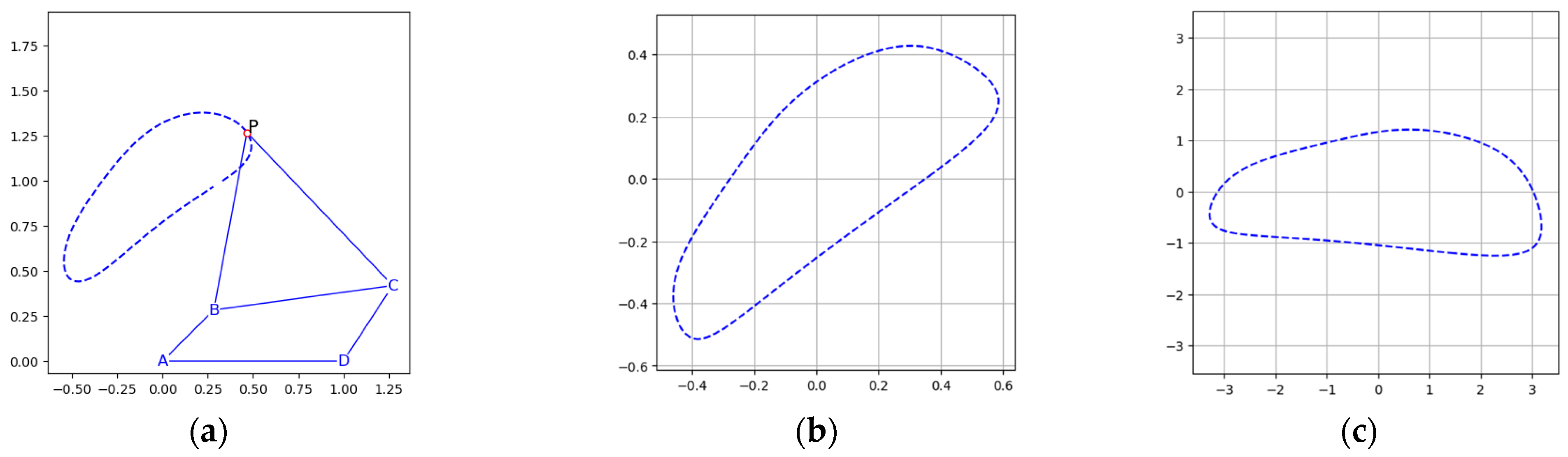
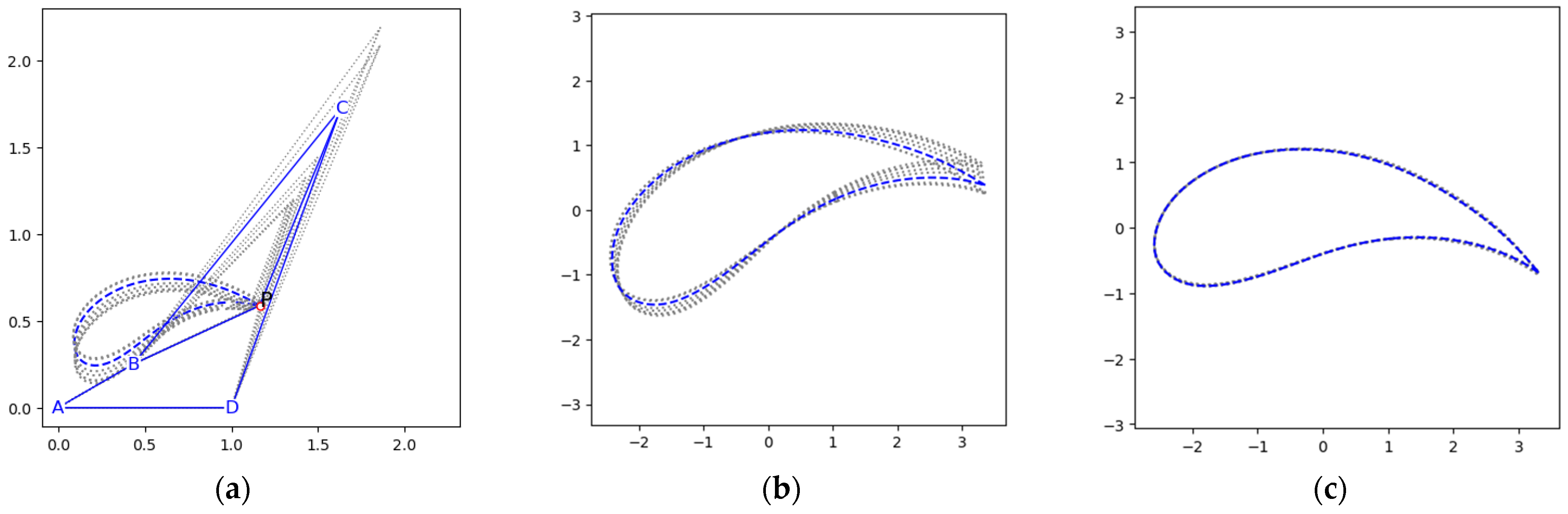
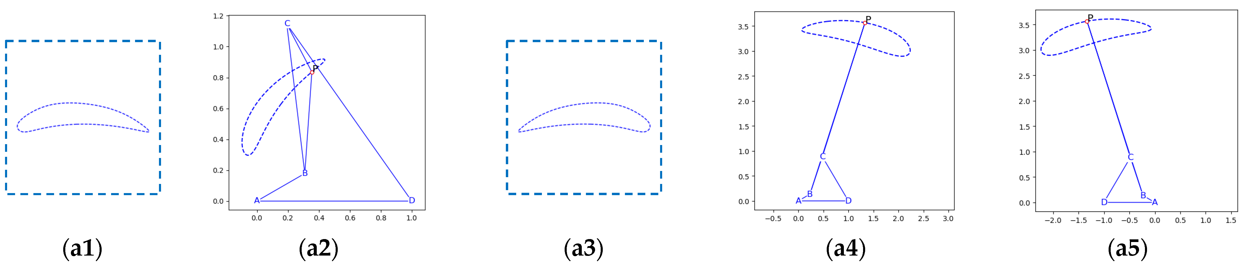
2.3. One-to-Many Mapping Issues

Although the Fourier descriptor approach can systematically represent the needs of the coupling problem, there remains one-to-many mapping in this synthesis problem. This implies that, for one input (a Fourier coefficient vector), there will be multiple output solutions (a set of linkage parameter vectors), as can be seen below:

(1)

Cognate linkages

According to the Roberts-Chebyshev theorem [34,35], for a trajectory curve that can be generated by a four-link mechanism, there are always three corresponding four-link mechanisms that describe the same curve. As shown in Figure 4, by drawing parallel lines and isoproportion lines to assist the analysis, one can get (a)–(c) parallelograms and (d), (e) reciprocal triangles of equal proportions A-P-B and then obtain the four-link system O-A-B-C-P, O-A’-E-O’-P and C-B’-F-O’-P with the same P-point trajectory curves. It also means the same Fourier coefficients, but with three different linkage parameters and configurations.

(2)

Factors of normalization

Due to the normalization, trajectory curves with different translations, rotations and scales, but with the same shape, will have the same Fourier coefficients.

(3)

Incomplete coupling at precise points

Multiple solutions arise regardless of whether there are too many or too few precise points coupled to the problem. When there are too few precise points, there are multiple different linkage trajectories to pass through, which is essentially a multi-solution paradigm. On the other hand, too many precise points may result in the inability to obtain a trajectory that perfectly passes through the precise points, and only approximate solutions can be obtained [36]. As shown in Figure 5, the different dashed lines are generated by using AD as the base reference and different combinations of other link parameters. These configurations are considered equivalent solutions within the allowable error after normalization.

As mentioned above, these aspects reveal that coupling curves will have multiple feasible solutions as a result of the one-to-many mappings, regardless of whether the coupler error falls within an acceptable range or is expressed in terms of the normalized Fourier coefficients.

2.4. Learning One-to-Many Mapping by Neural Networks

For problems with one-to-many mappings, the outputs corresponding to the same or similar inputs may vary significantly in the solution space near multiple solutions. This means that even small input variations can result in considerable output changes. The most straightforward case is to input the same Fourier coefficients and receive multiple different sets of linkages in the output, resulting in infinity variation. As a result, data models obtained using an ANN typically have poor learning quality.

Taking the Slider-Crank linkage shown in Figure 6 as an example, the relationship between the length $l$ and angle $\theta$ can be derived as follows:

$$l={\mathrm{r}}_{1}cos\theta +\sqrt{r_2^2-r_1^2{sin}^2\theta }.$$

(9)

Given the value of $l$, if one wishes to find the corresponding value of $\theta$, one needs to find the inverse solution of the equation. The geometric relationship symmetric to the vertical axis indicates the existence of two solutions. Therefore, a DNN designed to learn this inverse solution problem with $l$ as input and $\theta$ as output will contain a one-to-many mapping relationship (specifically, 1-to-2 in this case).

Table 2. Comparison of learning the $l-to-\theta$ mapping in the Slider-Crank mechanism.

Data Set Amount	Mean (Standard Deviation) of Prediction Errors			(Unit: rad)
	$$\mathit{\theta }:\left[-\frac{1}{2}\mathit{\pi },\frac{1}{2}\mathit{\pi }\right]$$	$$\mathit{\theta }:\left[-\frac{1}{4}\mathit{\pi },\frac{1}{2}\mathit{\pi }\right]$$	$$\mathit{\theta }:\left[0,\frac{1}{2}\mathit{\pi }\right]$$	$$\mathit{\theta }:\left[-\frac{1}{2}\mathit{\pi },0\right]$$
5000	0.7309 (0.0132)	0.3411 (*0.004)	0.0329 (0.0079)	0.0372 (0.0149)
10,000	0.7404 (0.0039)	0.3005 (0.0114)	0.0282 (0.0159)	0.0547 (0.0213)
50,000	0.7655 (0.0001)	0.2918 (0.0095)	0.0137 (0.0062)	0.0232 (0.0106)

* Remark: Bold numbers indicate the best scores.

shows that when the range of $\theta$ is restricted to the interval $\left[-1/2\pi ,1/2\pi \right]$, the learning quality is poor regardless of the size of the training set because each $l$ corresponds to two solutions; if the region of $\theta$ is restricted to the interval $\left[-1/2\pi ,1/4\pi \right]$, the quality is similarly poor due to the fact that multiple solutions still exist in the interval; and when the region of θ is restricted to the intervals $\left[0,1/2\pi \right]$ or $\left[-1/2\pi ,0\right]$, in which each $l$ value corresponds to a single $\theta$ solution, the trained DNN can obtain good learning results. As shown in the table, the prediction error can be reduced to about 1.8% in 50,000 data. In addition, when converging to one-to-one mapping relationship, the number of training sets increases to make DNN learning quality with significant improvement. Therefore, when employing a DNN approach to solve inverse problems, it is crucial to choose the solution space region thoughtfully and minimize one-to-many relationships.

In the past, studies using ANN to learn the synthesis have often improved the quality by restricting the parameter region of the linkages. However, it is typically challenging to directly analyze and derive appropriate constraints to limit the solution space to a small enough region to avoid multiple solutions in most practical inverse problems. On the other hand, solutions obtained by narrowing the parameter region are typically not able to meet the needs of general practical applications. This paper proposes using multiple DNNs to address this kind of inverse problem.

3. Synthesis Using Multiple DNNs

As mentioned above, it is necessary to establish the appropriate learning region for each DNN. However, since the synthesis is a complex nonlinear problem, it is difficult to obtain a complete solution landscape through analytical methods. On the other hand, previous research [37] has demonstrated the feasibility of investigating the multimodal solutions by restarter searches and obtaining optimal or far better solutions. Therefore, this paper proposes a multi-solution distribution evaluation by random restart local searches (MDE-RRLS) to assist the analysis of the solution space. MDE-RRLS analyzes the distribution of multiple solutions through sampling and generates a group of sub-datasets from the corresponding partitioned regions to train a set of DNNs. Figure 7 shows the overall learning and predicting process using MDE-RRLS as the evaluation metric, and the main steps in the process are explained as follows.

3.1. Dataset Partition and Generation for DNN Training Flow

Assuming that the normalized Fourier coefficients of the desired trajectory curve are $\overline{\mathrm{C}}=\left\{{\overline{c}}_{-d}\cdots {\overline{c}}_d\right\}$, the synthesis problem can be converted into the following optimization problem:

$$\min \sqrt{{\sum }_{n=-d, n\ne 0}^d{\left({\overline{c}}_n-{\overline{c}\prime }_n\right)}^2}$$

(10)

subject to ${\overline{C}}^{\prime }=\left\{{\overline{c}\prime }_{-d}\cdots {\overline{c}\prime }_d\right\}=\mathsf{\Gamma }\left(\mathsf{\phi },{\mathrm{r}}_2\cdots {\mathrm{r}}_5\right),\mathsf{\phi }\in \left[\mathrm{0,2}\pi \right],{\mathrm{r}}_k\in \left[{\widehat{\mathrm{r}}}_k,{\check{\mathrm{r}}}_k\right],$ and $2\le k\le 5$, where ${\overline{C}}^{\prime }$ is the coefficients of the trajectory curve of the predicted linkage mechanism, ${\widehat{\mathrm{r}}}_k$ and ${\check{\mathrm{r}}}_k$ are the lower and upper bounds of ${\mathrm{r}}_k$, respectively, and $\mathsf{\Gamma }\left(.\right)$ denotes as the Fourier transform and normalization function. Equation (10) tends to minimize the root mean square error (RMSE) of the desired and the predicted normalized coefficients. By encoding the linkage parameters into the objective function, this paper proposes a method for generating a set of coupling curves as samples. This method employs iteratively restarting and searching methods to explore the multi-solution locations of these samples and evaluates the relative merits of partitioning schemes. The evaluation is carried out by measuring the number of multi-solutions in the partitioned regions.

3.1.1. Multi-Solution Distribution Evaluation by Random Restart Local Searches (MDE-RRLS)

MDE-RRLS randomly generates M sets of linkage parameters as samples and converting them to normalized Fourier coefficients. Then, by searching the region in the entire solution space with a local search with randomly restarting L-1 times while trapped into a local solution. The goal of the search is to collect all the local solutions explored during the restart iterations. Since multiple solutions exist, the set of inverse solutions after repeatedly restarting searches is denoted as $\mathrm{S}=\left\{s_{i,j}|1\le i\le M,1\le j\le L\right\}$ where $s_{i,j}$ is the search result of the j-th partitioned region of the i-th sample, and its value is set to 0 if the solution is duplicated with the others or is not a feasible solution; otherwise, $s_{i,j}$ is set to the searched linkage parameter vector $\left[r_2,r_3,r_4,\phi ,r_5\right]$. MDE-RRLS computes and evaluates the number of multiple solutions that fall in the same partitioned region, which allows to discriminate the relatively better partition scheme.

In the implementation, MDE-RRLS computes the total number (labelled SUM) of the multiple solutions in a partition and the maximal amount (labelled MAX) of the multiple solutions in a partitioned region as the evaluation metrics, and the pseudo steps are shown in Algorithm 1.

Algorithm 1: MDE-RRLS

Input: $\mathrm{A} \mathrm{set} \mathrm{of} \mathrm{partitions} \mathrm{P}\mathrm{R}=\left\{{pr}_i|1\le i\le h\right\}$$\mathrm{where} h$$\mathrm{is} \mathrm{the} \mathrm{number} \mathrm{of} \mathrm{partitions} \mathrm{and} {pr}_i$ is the region covering the i-th partitioned $\mathrm{sub}\text{-}\mathrm{space} \mathrm{of} \left(\mathsf{\phi },{\mathrm{r}}_2\cdots {\mathrm{r}}_5\right)$. $\mathrm{A} \mathrm{set} \mathrm{of} \mathrm{explored} \mathrm{multi}-\mathrm{solutions} \mathrm{S}=\left\{s_{i,j}|1\le i\le M, 1\le j\le L\right\}$ after performing random local searches with restarting L-1 times when trapped. Output: SUM: total number of multi-solutions existed in the partitions. MAX: the maximal multi-solution number in a partitioned region.

Begin $\mathrm{Define} \mathrm{a} \mathrm{matrix} \mathrm{P}\mathrm{S}=\left[\begin{array}{ccc}{ps}_{\mathrm{1,1}}& \cdots & {ps}_{1,M}\\ \cdots & {ps}_{i,j}& \cdots \\ {ps}_{h,1}& \cdots & {ps}_{h,M}\end{array}\right]$$\mathrm{where} {ps}_{i,j}$ is the number of solutions of the j-th sample located at the i-th partitioned region and set as 0 initially. For k = 1 to h  For i = 1 to M   For j = 1 to L    $\mathbf{If} s_{i,j}$$\ne 0 \mathrm{and} s_{i,j}$$\mathrm{located} \mathrm{at} {pr}_k$$\mathbf{Then}\mathbf{,}\mathbf{ }{ps}_{i,j}$$={ps}_{i,j}$ + 1   Next j  Next i  For i = 1 to M   $\mathrm{If} {ps}_{k,i}$$\le 1 \mathrm{Then}, {ps}_{k,i}$ = 0   /* Count numbers only if more than one solution is in the same region */  Next i Next k   $\mathrm{Compute} SUM=\sum _{i=1}^h\sum _{j=1}^M{ps}_{i,j}.$ $\mathrm{Compute} MAX=\mathrm{the} \mathrm{maximum} \mathrm{of} \left\{\sum _{j=1}^M{ps}_{1,j}\cdots \sum _{j=1}^M{ps}_{h,j}\right\}$. End

Since all the sampled solutions will inevitably fall in all the partitioned regions, and between the partitioned regions, as illustrated in the Slider-Crank example above. It follows that learning quality increases when partitioned regions produce no or fewer multi-solutions. Consequently, a better partitioning scheme will have fewer SUM and MAX values. Using sampling can significantly reduce the computational cost compared to directly training the DNNs and then reviewing their learning quality.

3.1.2. Dataset Generation & Partition

After selecting the partition scheme, all linkage data within the partitioned region will be randomly generated. However, any data that does not satisfy the Grashof’s law or prohibits ${\mathrm{r}}_2$ from rotating by a full 360⁰ should be excluded. According to the sampling requirements of the Fourier transform, the sampling position $\left\{t_1\cdots t_{2d+1}\right\}$ is brought into P(t) to obtain the precise points $\left\{p_1\cdots p_{2d+1}\right\}$. Next, the Fourier coefficients are obtained after Fourier transformation and normalization. The dataset is then constructed by combining the Fourier coefficients with the parameters of the linkages to form an input-output pair ($\left[c_{-d}\cdots c_1\cdots c_d\right]$,$\left[{\mathrm{r}}_2,{\mathrm{r}}_3,{\mathrm{r}}_4,\phi ,{\mathrm{r}}_5\right]$). It should be noted that $c_0$ and ${\mathrm{r}}_1$ remain fixed throughout this process.

3.1.3. Training DNNs by Partitioned Datasets

Next, the dataset is partitioned into multiple sub-datasets based on the results of MDE-RRLS for training and learning purposes. The subsequent experiments also address the learning quality of DNNs trained using different partitioning schemes.

3.2. Predicting Flow to Obtain One or Multiple Solutions

When using the trained MDNNs for prediction, this paper proposes the multi-facet query (MFQuery) method which uses multiple projections of the desired curve to predict the outputs of the DNNs. In addition, since multiple DNNs are used to learn the overall solution space, when predicting the solutions, it is necessary to further cooperate with the trained DNNs to decide the most suitable solutions. Therefore, the paper also advocates for establishing a voting method for prediction.

3.2.1. Multi-Facet Query

For the desired curve, the standard method of prediction is sampling precise points and subsequently transforming and normalizing them into Fourier coefficients. Using these coefficients as the input, the trained DNNs will then predict the output of the corresponding linkage parameters. However, although the normalization effect allows the dataset to eliminate additional translations, scales, and rotations, there are still other affine transformations that have not been considered, such as vertical-axis versus horizontal-axis projection. There are two potential solutions to improve this problem. The first is to add additional affine transformations to the normalization of the dataset, but this approach will increase the number of multiple solutions again. The second solution involves transforming the desired coupler curve with the above two projections and querying the trained DNNs to predict additional linkages. Since the latter takes only a rather short time (usually less than 0.1 s) to perform the additional prediction, this paper proposes the second scheme to obtain more coupling candidate solutions within the same dataset.

MFQuery is implemented by first converting the normalized Fourier coefficients back to the sampling points (normalized precise points) of the curves and subsequently acquiring two additional sets of sampling points transformed by vertical-axis and horizontal-axis projections, followed by obtaining two additional sets of corresponding normalized Fourier coefficients. Then, the trained DNNs use these coefficient sets as inputs to predict the additional outputs (i.e., the linkage parameters), and finally, the best-fit solutions are chosen.

Figure 8 shows an MFQuery example. Figure 8(a1,b1) is the desired coupler curve. Figure 8(a3,b3) shows the curves after the projection of the vertical and horizontal axes, respectively. Additionally, Figure 8(a2,a4,b2,b4) is the prediction results of the trained DNNs, respectively. Since Figure 8(a4,b4) is the additionally projected linkages, the practical linkage configurations need to be applied with corresponding inverse projections; the resulting transformed configurations are shown in Figure 8(a5,b5).

In the presentation style, Figure 8(a1,b1) lacks specific axes since the axes can have arbitrary scales due to normalization. To ensure consistency, Figure 8(a3,b3) is presented following the same format as Figure 8(a1,b1), since they have a projection relationship with Figure 8(a1,b1).

3.2.2. Voting Method

Since synthesis can involve a single solution or a set of candidate solutions, a voting method is needed to select the best-fit solutions from the outputs of the trained DNNs. This paper employs the RMSE formulated in Equation (10) to assess the closeness of the trajectory points of output solutions to their corresponding precise point positions. All feasible solutions can be ranked according to the RMSE values, and the one with the lowest value can be selected, or an appropriate threshold can be set to reserve a collection of superior solutions.

4. Experiments and Discussions

In this section, the four-linkage-bar synthesis problem is first used to validate the proposed flows, and a comparison with the cases in the literature will also be made to identify the potential advantages of the proposed scheme. The following hardware and software specifications were used for the execution of the experiments: i7-12700 CPU, RTX4090 GPU, Windows 10 OS, and TensorFlow 2.

4.1. MDE-RRLS Evaluation and Selection of Subspace Partitions

In this test case, ${\mathrm{r}}_2,{\mathrm{r}}_3,{\mathrm{r}}_4,\phi ,{\mathrm{r}}_5$ parameters are used as the partition targets. Based on ${\mathrm{r}}_1=1$, the bar length ranges of ${\mathrm{r}}_2,{\mathrm{r}}_3,{\mathrm{r}}_4,{\mathrm{r}}_5$ are set to be [0.1, 3.5], and $\phi \in \left[\mathrm{0,2}\pi \right]$. In addition, according to the transmission angle μ (as shown in Figure 1a) is greater than or less than 90 degrees, the linkages can be assembled into different two kinds of configurations, “elbow-up “ and “elbow-down”, denoted as CFG to represent these two types with values 0 and 1. CFG is also used as the partition target. The Fourier transform is performed with a set of nine precise points to retain the first nine coefficients $\left(d=4\right)$ as chosen in [17].

Firstly, the distribution of multiple solutions in different partitioned regions was evaluated by MDE-RRLS in 100 samples (M = 100) where the sequential least squares programming method (SLSQP) [38] is employed in the local searches with 100 restarting times (L = 100). Then, further refined partitioning schemes were selected to review the changes in the distribution.

Table 3. MDE-RRLS evaluation results for the solution space partitions.

2 Regions	MAX (SUM)
* r2:2	55 (100)
r3:2	57 (72)
r4:2	56 (71)
Ψ:2	13 (22)
r5:2	55 (76)
CFG:2	15 (25)
4 Regions	MAX (SUM)
Ψ:4	6 (11)
Ψ:2, CFG:2	3 (6)
8 Regions	MAX (SUM)
Ψ:4, CFG:2	2 (6)
Ψ:8	2 (6)

* Remark: The partitioning setup is shown as (parameter):(partitioned region number).

shows the results of the MDE-RRLS evaluation with up to 8 partitioned regions. Firstly, the smallest SUM and MAX values obtained by MDE-RRLS were selected after comparing the cases with two equal regions, the top two being Ψ and CFG, respectively; and then the cases with four equal regions was performed to compare the two parameters including an individual partition (Ψ:4) and a combined partition (Ψ:2, CFG:2). Comparisons show that the obtained values decrease significantly in a larger number of regions, and in addition, the combined partition scheme leads to better values; finally, based on the SUM and MAX values, the case (Ψ:4, CFG:2) containing a quadratic partition in Ψ combined with an equal partition in CFG is selected here as the partitioning and learning blueprint for the subsequent training of DNNs.

4.2. Training Parameter Selection

For each partitioned sub-dataset, an individual DNN will be trained. Due to the stochastic nature of DNN learning and training, the mean and standard deviation of the 10 execution runs in each case are used as a basis for comparison. Other training parameters were set as follows: according to the number of data ranging from [0, 50,000], (50,000, 200,000], (200,000, 800,000] to (800,000, 1,600,000], the number of hidden layers and the number of neurons were combined to be (2, 32), (3, 64), (3, 128), and (4, 128), respectively. The activation function was the rectified linear unit function (ReLU) [39], the learning rate is 0.001 and the epoch number was 50.

Table 4. Comparison of learning quality of trained DNNs.

Data Amount	RMSE of Predictions in Different Partition Methods						Mean (std)
	Ψ:2	CFG:2	Ψ:4	Ψ:2, CFG:2	Ψ:8	Ψ:4, CFG:2	No Partition
80,000	0.5597 (0.0423)	0.596 (0.0302)	0.5349 (0.0202)	*0.5138 (0.0131)	0.5552 (0.0222)	0.5162 (0.0223)	1.4377 (0.0496)
400,000	0.3298 (0.023)	0.4262 (0.0301)	0.2866 (0.0261)	0.2758 (0.0171)	0.3212 (0.013)	0.2922 (0.014)	1.3279 (0.0367)
800,000	0.277 (0.0167)	0.3286 (0.0296)	0.2296 (0.0125)	0.232 (0.0244)	0.2488 (0.011)	0.2368 (0.0132)	1.2264 (0.0382)
1,600,000	0.2452 (0.0181)	0.2725 (0.0244)	0.2197 (0.0182)	0.2139 (0.0227)	0.2114 (0.0075)	0.2061 (0.0148)	1.1914 (0.0262)

* Remark: Bold numbers indicate the best scores.

compares the learning results after training of DNNs, and it can be observed that when 8 DNNs are learned cooperatively, the average prediction error of (Ψ:4, CFG:2) is better; and when the number of datasets is increased, the overall quality of learning is also improved.

In addition, Table 4 also shows that the quality of learning tends to be similar to the assessed values for the various MDE-RRLS outcomes shown in Table 3. When the dataset is large enough, the results tend to be more consistent. Moreover, when the number of partitions reaches a certain number, the decrease in prediction error becomes less obvious, and this effect also reflect in the evaluation of MDE-RRLS. Thus, the MDE-RRLS evaluation can guide the partitioning of the dataset, resulting in an improved quality of learning.

It should be noted that even if the data number increases, none of the single neural network solutions in scheme (No Partition) can get good solution quality. Even with the largest dataset in the table, the average error is still five times higher compared to the partitioning scheme (Ψ:4, CFG:2) for the same dataset.

4.3. Comparison with Literature Cases

To verify the results of the proposed approach, a previous four-linkage-bar synthesis case [17] is used here for a comparative study. In the original study, both the setup in Figure 9 was chosen with the origin as A and AD coinciding with the x-axis, which is equivalent to Figure 1a. For the sake of fairness, the other setting as that of the previous work is also used, where the information of the linkage parameters is defined in terms of the endpoint coordinates of the link-bars, e.g., the coordinates of the joint A point are denoted as $\left(x_A,y_A\right)$. In addition, datasets of the same size (i.e., 60,000 data volume) were used.

It should be noted that the original study used a single ANN as the solution method; however, as mentioned above, datasets with multiple solutions will make the ANN training converge poorly. Therefore, the original study restricted parameter ranges to a limited region where the link-bar scale is small, the inverse solution exists, and the mechanism will not get stuck in the simulation. The conditional rule enhances the coupling success rate, but its extensiveness can be relatively limited (e.g., the selected parameter region will only produce Crank-Rocker bodies).

In this synthesis problem, eight DNNs are trained using the partition scheme mentioned earlier (Ψ:4, CFG:2). Figure 10 shows the comparison between the proposed multi-DNNs scheme and the results of the previous work, where the scheme proposed in this paper obtains better solutions in the first and second cases and comparable solutions in the third and fourth cases. Figure 11 shows that the MFQuery method obtains additional good solutions after making predictions using vertical and horizontal projection curves, and the more suitable solutions are selected by the boxes. In the second and fourth cases, the queries by projection curves obtain obviously better coupling solutions compared to the original curve.

The output (linkage) parameters obtained in this study are shown in

Table 5. Synthesis results for linkage parameters.

Study Cases	${\mathit{\theta }}_1$	r1	r2	r3	r4	$\mathsf{\phi }$	r5	CFG	Projection
#1	−0.52	234.23	64.62	249.61	360.60	4.22	163.67	0	None
#2	−0.27	135.82	35.68	246.41	265.25	0.02	358.53	0	Horizontal
#3	−0.45	299.31	76.90	361.66	402.66	4.71	298.47	0	None
#4	−0.19	234.23	85.09	260.69	141.45	0.36	230.54	0	Horizontal

. Although the impact of ${\theta }_1$ variation vanishes after the normalization process, inverse normalization is still required for an inverse rotation during the final coupling stage, with the amount of rotation provided by ${\theta }_1$.

5. Application to Design an Industrial Six-Bar Ladle Mechanism

To verify the effectiveness of the proposed method in practical applications, this paper discusses how to expand the application of the proposed method in practical cases through a six-linkage-bar mechanism design case. As illustrated in Figure 12, this mechanism is used for metal-mold die-casting system in loading the liquid metal [22], and in the actual production, ${\theta }_1$ is driven by an electric motor, and the tail end will be configured with a soup spoon. As shown in Figure 12c, while the OU bar is rotating, the mechanism loads the liquid metal (such as aluminum liquid) from the boiler, moves around the boiler wall, and finally arrives at the location of the pouring hole.

Based on this operational requirement, the precise points need to be designed to pass through the motion path of F-point in Figure 12c, in order to couple the required linkage synthesis design parameters.

In the kinematic derivation part, due to the fixation of pivot points O and C, the mechanism is constrained to one degree of freedom. The position of the F-point can be derived by extending the aforementioned four-linkage case, which can finally be expressed as the relationship equations of $\left[{\mathrm{c}}_x,{\mathrm{c}}_y,{\mathrm{r}}_1,{\mathrm{r}}_2,{\mathrm{r}}_3,{\mathrm{r}}_4,{\mathrm{r}}_5,{\mathrm{r}}_6,{\mathrm{r}}_7\right]$ and ${\theta }_1$ in Figure 12c diagram, and the detailed derivation process can be referred to [32].

Unlike the previous four-linkage-bar synthesis problem, the difficulty of coupling the six-linkage-bar increases due to the increase in the number of linkage parameters. In addition, the operation path of this six-bar mechanism is mainly a back-and-forth iterative motion between the loading and the pouring positions, which differs from the previous four-bar case by not being a closed curve. Consequently, it cannot be directly converted by the previous Fourier transform and normalization. In this case, this paper proposes to preprocess the original non-closed curve into a closed curve by a geometric projection, before applying the same solution process to achieve synthesis design.

5.1. Design Precise Points and Partition Schemes

As shown in Figure 12b, five precise points {(290,−1398), (113,−1088), (−518,−815), (−1009,−680), (−1229,−919)} which are then projected onto the reference axis to form a closed curve. This results in obtaining nine symmetrical points after mapping once the duplicate starting endpoints have been subtracted. The Fourier transform is subsequently performed using this set of precise points, with the first nine coefficients $\left(d=4\right)$ being retained.

In the experiments, ${\mathrm{c}}_x=100$ was used as the base size, and for other linkage parameters containing ${\mathrm{c}}_y,{\mathrm{r}}_1,{\mathrm{r}}_2,{\mathrm{r}}_3,{\mathrm{r}}_4,{\mathrm{r}}_5,{\mathrm{r}}_6$ and ${\mathrm{r}}_7$, their ranges are set as [300,500], [100,3000], [100,3000], [100,3000], [100,3000], [100,3000], [100,3000] and [100,3000], respectively; and the partition schemes were compared by MDE-RRLS.

Table 6. Comparison of partitioning methods for six-linkage-bar parameters.

2 Regions	MAX (SUM)
Cy:2	28 (32)
r1:2	16 (28)
r2:2	23 (26)
r3:2	17 (23)
r4:2	20 (25)
r5:2	19 (22)
r6:2	13 (18)
r7:2	*9 (14)
4 Regions	MAX (SUM)
r7:4	3 (8)
r7:2, r6:2	3 (6)
8 Regions	MAX (SUM)
r7:4, r6:2	1 (2)
r7:8	2 (6)

* Remark: The partitioning setup is shown as (parameter):(partitioned region number).

shows the MAX and SUM values evaluated with 100 samples; observing the result, the use of (r7:4, r6:2) is a better partition scheme.

5.2. Multi-DNNs Training Results

Next, a dataset of 1,600,000 data is created and partitioned into eight equal regions in partition (r7:4, r6:2), and each sub-dataset is used to train one DNN, respectively.

Table 7. Prediction results of the trained DNNs.

DNN No	ox	oy	cx	cy	r1	r2	r3	r4	r5	r6	r7
1	13.92	92.89	186.72	615.26	219.84	498.5	323.27	1427.38	452.83	1058.51	964.14
2	62.56	186.41	215.45	710.56	207.65	467.71	301.6	1367.77	451.54	910.34	1088.36
3	95.67	115.96	186.42	618.8	203.89	438.73	259.53	1851.51	550.87	1393.61	1597.08
4	114.26	176.75	210.67	690.03	200.5	426.18	297.89	1505.03	450.45	1045.28	1530.64
5	4.78	246.23	217.5	709.54	194.58	469.81	305.44	1352.53	347.01	1081.34	725.82
6	18.19	234.81	212.45	714.23	197.21	475.72	321.05	1486.01	391.81	1094.67	1129.86
7	93.63	358.67	263.03	862	188.17	447.75	296.24	1470.82	371.21	1051.77	1210.44
8	37.82	133.99	213.72	684.79	222.4	503.03	331	1319.76	334.43	791.37	1208.21

shows the results of the eight trained DNNs. Notably, the values of $o_x$, $o_y$, and $c_x$ obtained via inverse normalization are presented despite their omission from the DNN training parameters. they are the corresponding values obtained from the inverse normalization. Figure 13 shows the trajectory curves of each solution, with the markers in the upper half of the curve being the desired precise point locations. In addition, since this problem is a practical application and the design of the mechanism does not allow for vertically or horizontally projected installation, only the original trajectory curves from MFQuery are used to predict the linkage parameters in this design problem.

Figure 14 shows the better solutions 2, 4 and 6, respectively, which contain each linkage configuration with its corresponding trajectory curve. Observing the motion curves in the figure, the trajectory curves are close to the desired precise points. Therefore, the design requirements can be achieved, and the other solutions, such as solutions 3, 7 and 8, are also solutions that can be considered with some fine-tuning if only the loading and injection points are the focal points.

5.3. Design Refinement in a Short-Time Response

Since the trained DNNs can compute (predict) the output linkage parameters quite quickly, the proposed scheme can respond fast to the linkage redesign with the change of the precise points. Figure 15 shows that the corresponding design is obtained by simulating the drag-and-move interactive design when a precise point is moved from A-point to B-point, where four consecutive changes are made. Due to the fast computation capabilities of the trained DNNs (the computation time is less than 1 s in the tested environment), their performance can be applied to applications that require a short response time, which can provide designers with considerable real-time options.

6. Conclusions

The linkage synthesis problem described by the Fourier descriptor and normalization allows for a systematic representation of coupled trajectory curves. However, a single neural network for synthesizing methods results in poor learning quality due to multiple solutions existing in the dataset. Therefore, this paper proposes using the MDE-RRLS method to enhance the partition scheme of the solution space, employing multiple DNNs to learn the partitioned subspaces, and using the MFQuery method on the trained DNNs to predict additional candidate solutions. Finally, the candidate solutions are combined to obtain a single optimal solution by the voting method or multiple feasible solutions by a threshold.

By comparing with the four-linkage-bar synthesis cases in the literature, the proposed scheme can obtain better or at least competitive solutions. When applied to the design of an industrial six-bar ladle mechanism, the proposed approach can successfully synthesize several candidate solutions by applying the proposed partition and training processes. Additionally, when the six-bar ladle requires redesigning due to local path changes, the proposed approach can successfully obtain a feasible solution in a rather short time through the cooperation of multiple DNNs.

References

1. Li, X.; Wei, S.; Liao, Q.; Zhang, Y. A Novel Analytical Method for Function Generation Synthesis of Planar Four-Bar Linkages. Mech. Mach. Theory 2016, 101, 222–235. [Google Scholar] [CrossRef]
2. Calvetti, D.; Somersalo, E. Inverse Problems: From Regularization to Bayesian Inference. Wiley Interdiscip. Rev. Comput. Stat. 2018, 10, e1427. [Google Scholar] [CrossRef]
3. Lee, W.-T.; Russell, K. Developments in Quantitative Dimensional Synthesis (1970–Present): Four-Bar Path and Function Generation. Inverse Probl. Sci. Eng. 2018, 26, 1280–1304. [Google Scholar] [CrossRef]
4. Hernández, A.; Muñoyerro, A.; Urízar, M.; Amezua, E. Comprehensive Approach for the Dimensional Synthesis of a Four-Bar Linkage Based on Path Assessment and Reformulating the Error Function. Mech. Mach. Theory 2021, 156, 104126. [Google Scholar] [CrossRef]
5. Cabrera, J.; Simon, A.; Prado, M. Optimal Synthesis of Mechanisms with Genetic Algorithms. Mech. Mach. Theory 2002, 37, 1165–1177. [Google Scholar] [CrossRef]
6. Halicioglu, R.; Jomartov, A.; Kuatova, M. Optimum Design and Analysis of a Novel Planar Eight-Bar Linkage Mechanism. Mech. Based Des. Struct. Mach. 2023, 51, 5231–5252. [Google Scholar] [CrossRef]
7. Liu, X.; Ding, J.; Wang, C. Design Framework for Motion Generation of Planar Four-Bar Linkage Considering Clearance Joints and Dynamics Performance. Machines 2022, 10, 136. [Google Scholar] [CrossRef]
8. Eqra, N.; Abiri, A.H.; Vatankhah, R. Optimal Synthesis of a Four-Bar Linkage for Path Generation Using Adaptive PSO. J. Braz. Soc. Mech. Sci. Eng. 2018, 40, 469. [Google Scholar] [CrossRef]
9. Sancibrian, R.; Sedano, A.; Sarabia, E.G.; Blanco, J.M. Hybridizing Differential Evolution and Local Search Optimization for Dimensional Synthesis of Linkages. Mech. Mach. Theory 2019, 140, 389–412. [Google Scholar] [CrossRef]
10. Acharyya, S.; Mandal, M. Performance of EAs for Four-Bar Linkage Synthesis. Mech. Mach. Theory 2009, 44, 1784–1794. [Google Scholar] [CrossRef]
11. Jiang, C.; Liu, G.; Han, X. A Novel Method for Uncertainty Inverse Problems and Application to Material Characterization of Composites. Exp. Mech. 2008, 48, 539–548. [Google Scholar] [CrossRef]
12. Pathak, V.K.; Singh, R.; Sharma, A.; Kumar, R.; Chakraborty, D. A Historical Review on the Computational Techniques for Mechanism Synthesis: Developments Up to 2022. Arch. Comput. Methods Eng. 2023, 30, 1131–1156. [Google Scholar] [CrossRef]
13. Galán-Marín, G.; Alonso, F.J.; Del Castillo, J.M. Shape Optimization for Path Synthesis of Crank-Rocker Mechanisms Using a Wavelet-Based Neural Network. Mech. Mach. Theory 2009, 44, 1132–1143. [Google Scholar] [CrossRef]
14. McGarva, J.; Mullineux, G. Harmonic Representation of Closed Curves. Appl. Math. Model. 1993, 17, 213–218. [Google Scholar] [CrossRef]
15. Sharma, S.; Purwar, A.; Jeffrey Ge, Q. An Optimal Parametrization Scheme for Path Generation Using Fourier Descriptors for Four-Bar Mechanism Synthesis. J. Comput. Inf. Sci. Eng. 2019, 19, 014501. [Google Scholar] [CrossRef]
16. Hoskins, J.C.; Kramer, G.A. Synthesis of Mechanical Linkages Using Artificial Neural Networks and Optimization. In Proceedings of the IEEE International Conference on Neural Networks, San Francisco, CA, USA, 28 March–1 April 1993; p. 822-J. [Google Scholar]
17. Vasiliu, A.; Yannou, B. Dimensional Synthesis of Planar Mechanisms Using Neural Networks: Application to Path Generator Linkages. Mech. Mach. Theory 2001, 36, 299–310. [Google Scholar] [CrossRef]
18. Khan, N.; Ullah, I.; Al-Grafi, M. Dimensional Synthesis of Mechanical Linkages Using Artificial Neural Networks and Fourier Descriptors. Mech. Sci. 2015, 6, 29–34. [Google Scholar] [CrossRef]
19. Li, X.; Chen, P. A Parametrization-Invariant Fourier Approach to Planar Linkage Synthesis for Path Generation. Math. Probl. Eng. 2017, 2017, 8458149. [Google Scholar] [CrossRef]
20. Li, X.; Epitropakis, M.G.; Deb, K.; Engelbrecht, A. Seeking Multiple Solutions: An Updated Survey on Niching Methods and Their Applications. IEEE Trans. Evol. Comput. 2016, 21, 518–538. [Google Scholar] [CrossRef]
21. Deshpande, S.; Purwar, A. A Machine Learning Approach to Kinematic Synthesis of Defect-Free Planar Four-Bar Linkages. J. Comput. Inf. Sci. Eng. 2019, 19, 021004. [Google Scholar] [CrossRef]
22. Chen, C.-H.; Liu, T.-K.; Huang, I.-M.; Chou, J.-H. Multiobjective Synthesis of Six-Bar Mechanisms under Manufacturing and Collision-Free Constraints. IEEE Comput. Intell. Mag. 2012, 7, 36–48. [Google Scholar] [CrossRef]
23. Xie, J.; Chen, Y. Application Back Propagation Neural Network to Synthesis of Whole Cycle Motion Generation Mechanism. In Proceedings of the 12th IFToMM World Congress-Besancon-France, Besançon, France, 17–21 June 2007. [Google Scholar]
24. Erkaya, S.; Uzmay, I. Optimization of Transmission Angle for Slider-Crank Mechanism with Joint Clearances. Struct. Multidiscip. Optim. 2009, 37, 493–508. [Google Scholar] [CrossRef]
25. Ahmadi, B.; Nariman-zadeh, N.; Jamali, A. Path Synthesis of Four-Bar Mechanisms Using Synergy of Polynomial Neural Network and Stackelberg Game Theory. Eng. Optim. 2017, 49, 932–947. [Google Scholar] [CrossRef]
26. Mo, X.; Ge, W.; Zhao, D.; Zhang, Y. Path Synthesis of Crank-Rocker Mechanism Using Fourier Descriptors Based Neural Network. In Recent Advances in Mechanisms, Transmissions and Applications, Proceedings of the Fifth MeTrApp Conference 2019; Springer: Singapore, 2020; pp. 32–41. [Google Scholar]
27. Yim, N.H.; Lee, J.; Kim, J.; Kim, Y.Y. Big Data Approach for the Simultaneous Determination of the Topology and End-Effector Location of a Planar Linkage Mechanism. Mech. Mach. Theory 2021, 163, 104375. [Google Scholar] [CrossRef]
28. Kapsalyamov, A.; Hussain, S.; Brown, N.A.; Goecke, R.; Hayat, M.; Jamwal, P.K. Synthesis of a Six-Bar Mechanism for Generating Knee and Ankle Motion Trajectories Using Deep Generative Neural Network. Eng. Appl. Artif. Intell. 2023, 117, 105500. [Google Scholar] [CrossRef]
29. Yim, N.H.; Ryu, J.; Kim, Y.Y. Big Data Approach for Synthesizing a Spatial Linkage Mechanism. In Proceedings of the 2023 IEEE International Conference on Robotics and Automation (ICRA), London, UK, 29 May–2 June 2023; pp. 7433–7439. [Google Scholar]
30. Norton, R.L. Fundamentals of Machine Design; McGraw-Hill: New York, NY, USA, 2004. [Google Scholar]
31. Wandling Sr, G.R. Synthesis of Mechanisms for Function, Path, and Motion Generation Using Invariant Characterization, Storage and Search Methods; Iowa State University: Ames, IA, USA, 2000. [Google Scholar]
32. Yan, H.S. Mechanisms: Theory and Applications, 1st ed.; McGraw Hill Education (Asia): Singapore, 2016; ISBN 978-981-4660-00-6. [Google Scholar]
33. Li, X.; Wei, S.; Liao, Q.; Zhang, Y. A Novel Analytical Method for Four-Bar Path Generation Synthesis Based on Fourier Series. Mech. Mach. Theory 2020, 144, 103671. [Google Scholar] [CrossRef]
34. Sherman, S.N.; Hauenstein, J.D.; Wampler, C.W. A General Method for Constructing Planar Cognate Mechanisms. J. Mech. Robot. 2021, 13, 031009. [Google Scholar] [CrossRef]
35. Roberts, S. On Three-Bar Motion in Plane Space. Proc. Lond. Math. Soc. 1875, 1, 14–23. [Google Scholar] [CrossRef]
36. Kang, Y.-H.; Lin, J.-W.; You, W.-C. Comparative Study on the Synthesis of Path-Generating Four-Bar Linkages Using Metaheuristic Optimization Algorithms. Appl. Sci. 2022, 12, 7368. [Google Scholar] [CrossRef]
37. Lourenço, H.R.; Martin, O.C.; Stützle, T. Iterated Local Search: Framework and Applications. In Handbook of Metaheuristics; Springer: Boston, MA, USA, 2019; pp. 129–168. [Google Scholar]
38. Virtanen, P.; Gommers, R.; Oliphant, T.E.; Haberland, M.; Reddy, T.; Cournapeau, D.; Burovski, E.; Peterson, P.; Weckesser, W.; Bright, J.; et al. SciPy 1.0: Fundamental Algorithms for Scientific Computing in Python. Nat. Methods 2020, 17, 261–272. [Google Scholar] [CrossRef]
39. Dubey, S.R.; Singh, S.K.; Chaudhuri, B.B. Activation Functions in Deep Learning: A Comprehensive Survey and Benchmark. Neurocomputing 2022, 503, 92–108. [Google Scholar] [CrossRef]
40. Chen, C.-H.; Liu, T.-K.; Chou, J.-H. A Novel Crowding Genetic Algorithm and Its Applications to Manufacturing Robots. IEEE Trans. Ind. Inform. 2014, 10, 1705–1716. [Google Scholar] [CrossRef]
Figure 1. Coordinate system and parameters of a four-linkage-bar. (a) Simplified structure diagram. (b) General analysis diagram.
Machines 11 01018 g001
Figure 2. Example of the normalized trajectory curve of a linkage-bar. (a) Original P-point trajectory. (b) Translation normalization by zeroing c 0 . (c) Scale and rotation normalization by standardizing the value of c 1 .
Machines 11 01018 g002
Figure 3. Synthesizing the mapping between Fourier coefficients and linkage parameters.
Machines 11 01018 g003
Figure 4. Cognate linkages [35].
Machines 11 01018 g004
Figure 5. Normalization effect in Fourier-series representation. (a) Example linkages. (b) Translated & scaled linkages. (c) Complete normalization.
Machines 11 01018 g005
Figure 6. Coordinate system and parameters of a Slider-Crank mechanism. (a) A Slider-Crank mechanism. (b) Analysis diagram.
Machines 11 01018 g006
Figure 7. Proposed DNN learning and predicting flows. (a) Dataset partition and generation for DNN training flow. (b) Predicting Flow to Obtain One or Multiple Solutions.
Machines 11 01018 g007
Figure 8. Multi-facet query example flows. (a1) Desired curve. (a2) Solution by querying the desired shape. (a3) Vertical-axis projected curve. (a4) Querying the projected shape. (a5) Solution after inverse projection. (b1) Desired curve. (b2) Solution by querying the desired shape. (b3) Horizontal-axis projected curve. (b4) Querying the projected shape. (b5) Solution after inverse projection.
Machines 11 01018 g008aMachines 11 01018 g008b
Figure 9. Setting in the previous four-linkage-bar synthesis [17].
Machines 11 01018 g009
Figure 10. Comparison results of the four-linkage-bar synthesis problem. (a) Study Case #1. (b) Study Case #2. (c) Study Case #3. (d) Study Case #4.
Machines 11 01018 g010
Figure 11. Multi-facet query results.
Machines 11 01018 g011
Figure 12. Coordinate system and parameters of the six-bar ladle mechanism. (a) Ladle mechanism [40]. (b) Operation diagram. (c) Structure analysis diagram.
Machines 11 01018 g012
Figure 13. Trajectory curves predicted by multiple trained DNNs. (a) Prediction in DNN #1. (b) Prediction in DNN #2. (c) Prediction in DNN #3. (d) Prediction in DNN #4. (e) Prediction in DNN #5. (f) Prediction in DNN #6. (g) Prediction in DNN #7. (h) Prediction in DNN #8.
Machines 11 01018 g013
Figure 14. Example linkage solutions from the different trained DNNs. (a) Linkage structure in DNN #2. (b) Linkage structure in DNN #4. (c) Linkage structure in DNN #6.
Machines 11 01018 g014
Figure 15. Redesign case due to local path changes.
Machines 11 01018 g015