Abstract
The fault feature extraction and diagnosis of autonomous underwater vehicles (AUVs) in complex environments pose significant challenges due to the intricate nature of the signals that reflect the AUVs’ states in the deep ocean. In this paper, an analytical model-free fault diagnosis algorithm based on a multi-channel full convolutional neural network (MC-FCNN) is introduced to establish patterns between AUV states and potential fault types using multi-sensor signals. Firstly, the AUV raw dataset undergoes random forest multiple imputation by chained equations (RF-MICE) to serve as the input of the convolution neural network. Next, signal features are extracted through the full convolution channel, which can be fused as multilayer perceptron (MLP) input and Softmax classifier for fault identification. Finally, to validate the effectiveness of the proposed MC-FCNN model, fault diagnosis experiments are conducted using the dataset sourced from the Zhejiang University Laboratory with missing data. The experimental results demonstrate that, even with of the data missing, the proposed RF-MICE with MC-FCNN model can still achieve an ideal fault identification.
1. Introduction
Autonomous underwater vehicles (AUVs) play crucial and irreplaceable roles in the exploration and utilization of ocean resources and space, which are increasingly utilized as tools for oceanic reconnaissance and deep-sea work at present. As the security and reliability of deep-sea engineering equipment become more significant, there has recently been a growing focus on AUV fault diagnosis techniques both domestically and internationally.
With the advancements in data-driven [1] and artificial intelligence techniques [2,3], the analysis of complex data using machine learning approaches has emerged as a critical research field in AUV fault diagnosis [4]. For instance, an evidence theory and normalization-based feature extraction and fusion method for AUV thruster fault diagnosis was proposed in Ref. [5]. In addition, support vector machine (SVM) [6], a statistical learning theory-based machine learning technique, has been employed to analyze convergence speed and learning consistency based on the principle of structure risk minimization. In Ref. [7], a fuzzy SVM-based method for multiple fault diagnosis in AUVs was proposed. This method aimed to enhance fault classification accuracy by incorporating local sparsity and category weights for each sample. However, the reliance on expertise capture in feature extraction restricted its applicability, and the shallow network structure limited the deep extraction in fault features.
In order to address the aforementioned problems, there is a growing interest in the field of deep learning theory-based intelligent fault diagnosis [8,9,10]. Ref. [11] proposed a fault diagnosis method for AUV thrusters by combining a locally approximated cerebellar network model and fuzzy control for fault diagnosis modeling. Ref. [12] proposed a fault detection and diagnosis scheme for underwater thrusters using a recurrent neural network nominal model based on empirical data. The above studies effectively tackled the challenge of AUV modeling using deep learning models, which has historically been difficult due to the complex nonlinear dynamics of the deep-sea environment. At present, the convolutional neural network (CNN)-based research on AUV fault diagnosis is still at the stage of theoretic exploration, with some relevant attempts already made [13,14,15,16]. In Ref. [17], a fault diagnosis method for AUVs based on a sequential convolutional neural network was proposed, utilizing raw AUV state data as input. This method not only removes the limitations on feature extraction in existing work but also possesses adaptive feature extraction capabilities and end-to-end characteristics. Hence, deep learning theory can be effectively applied on AUV fault diagnosis in complex working conditions.
However, in the deep-sea environment, the performance of AUV fault diagnosis using a convolutional neural network can be compromised when sensor signals are missing. This is because neural networks are unable to accurately output diagnosis results when their inputs contain missing data. As a result, there is an urgent need for imputation methods in AUV fault diagnosis based on neural networks to estimate the missing sensor data. The commonly used data imputation methods include mean imputation, k-nearest neighbor (KNN) imputation, regression imputation, and so on [18,19]. The regression-based imputation approach utilizes the relationships between the auxiliary variables and target variables to construct a regression model. This method yields better results when auxiliary variables are highly correlated with target variables. Compared with regression imputation, mean imputation often distorts the empirical distribution of samples, while the KNN imputation method heavily relies on data distribution. AUV state data typically exhibit multidimensionality, featuring complex and nonlinear relationships between variables. Consequently, traditional data imputation methods face challenges in handling such data. In recent years, with the rapid advancement of machine learning methods, imputation methods based on machine learning [20] have emerged. Among these methods, imputation methods utilizing random forest [21,22] have attracted attention from statisticians. Random forest-based imputation methods are capable of handling nonlinear relationships, higher-order correlations, and missing values by constructing multiple decision trees for imputation purposes.
Based on the aforementioned points, this paper proposes a solution to the problem of online data missing diagnosis by introducing a model-free multi-channel full convolutional neural network (MC-FCNN)-based AUV fault diagnosis scheme. This scheme combines the random forest multiple imputation method with the chained equations (RF-MICE [23,24]) technique for a more accurate diagnosis. Additionally, an end-to-end fault diagnosis framework based on a full convolutional network is implemented with multiple channel inputs, self-learning, and fusion capabilities. The remaining sections are organized as follows. Missing data estimation with the multiple imputation method is introduced in Section 2. The typical CNN model and one-dimensional convolutional neural networks (1D-CNNs) are introduced in Section 3. The proposed MC-FCNN architecture and fault diagnosis implementation are shown in Section 4. Experimental results and analysis are shown in Section 5. Conclusions and our future work are drawn in Section 6.
2. Missing Data Estimation with Multiple Imputation
2.1. Random Forest Algorithm
Random forest is an integrated learning method that addresses both classification and regression problems. The method works by constructing a large number of decision trees, and the output is determined by the combination of all the individual decision trees. In a classification problem, the final result is decided based on the maximum number of votes, whereas in a regression problem, the final result is predicted based on the mean value. By doing so, the random forest constructs each decision tree based on partial samples each time, effectively addressing the problem of overfitting in decision trees. Each decision tree in a random forest is a collection of training samples constructed by repeatedly conducting put-back sampling from the original dataset. During the process of building the decision tree, the input data undergo random sampling in both rows and columns. Row sampling allows for the possibility of duplicate samples in the collected sample set. This ensures that the input samples for each tree are not solely composed of all the samples during training, minimizing the risk of overfitting. Additionally, column sampling is performed to selectively choose certain features from the entire set of features in order to construct each decision tree. A full split strategy is employed, meaning that the leaf nodes of each decision tree are split until they can no longer be further divided. Overall, pruning is considered as a critical step in many decision tree algorithms; however, it is not utilized in this particular method. The combination of the two random sampling processes ensures randomness, thereby mitigating the risk of overfitting even in the absence of pruning.
The construction process of the random forest is as follows:
Step1: When constructing each decision tree, m samples are randomly selected from the original dataset with put-back sampling. The above process is repeated n times to train n decision tree models.
Step 2: In each random decision tree model, at each node of the decision tree split, n attributes are randomly chosen from the total of N attributes present in each sample, where n ≤ N. The Gini index is then used to select the best feature from these n attributes for the split.
Step 3: Each tree continues to grow by completing splits until the next node selects features that were already used in the split of its parent node. At this point, further splitting is unnecessary. Throughout the construction of the decision tree, no pruning is performed.
Step 4: The aforementioned steps are repeated to construct a significant number of decision trees, resulting in the creation of a comprehensive random forest model.
2.2. RF-MICE Technique
Random forest multiple imputation by chained equations is an effective approach for addressing the issue of missing data. It involves conducting multiple iterations of random forest prediction models on multiple series. The estimation of certain variables in the missing data is dependent on the values of other variables. Denote the original dataset with missing data as ; are k incomplete variables with missing data, are j complete variables without missing data, where . has a total number of variables and X are the variables to be imputed. Additionally, when j equals 0, this indicates that the original dataset does not contain any complete variables. The proposed method for random forest multiple imputation by chained equations can be outlined as follows. The process of multiple imputation by chained equations (also known as MICE [25]) involves iteratively fitting a predictive model for each variable with missing values, conditioned upon the other variables in the dataset. The detailed representation of this process is illustrated in Figure 1.
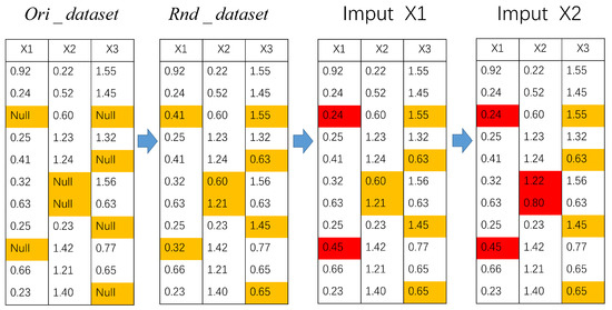
Figure 1.
Multiple imputation by chained equations (yellow: the missing values; red: the imputed values).
Step 1: For the original dataset with missing data , denote the reconstructed dataset based on the multiple imputation method for missing values as . In this dataset, the missing values are imputed using random values from the current variable.
Step 2-a: Take of as the label column, and the attributes alongside in as the feature matrix. The training set consists of the samples corresponding to the non-missing values in , while the test set involves the samples corresponding to the missing values in . Based on this, a random forest model is constructed and the missing value can be predicted.
Step 2-b: Following the similar step as described above, take of as the label column. The feature matrix for this step consists of from the , where has been imputed. Repeat step 2-a until all the incomplete attributes of X in are updated with missing value in a single iteration.
Step 3: Stop the process after n iterations of step 2 (steps 2-a and 2-b) and output the final complete dataset . In each iteration, the updated values of the other variables from the previous round are taken as the feature matrices, while the current variables to be imputed in the are considered as the label column.
Step 4: Repeat the previous steps 1-3 m times in order to obtain m complete datasets.
By employing the multiple imputation method, missing values in the crossover design can be imputed while considering the associated uncertainty. This approach allows for the generation of valid statistical inferences. In particular, the random forest multiple imputation by chained equations technique proposed in this study can effectively handle mixed types of nonlinear data. Furthermore, it has the capability to impute data for both continuous and categorical variables simultaneously. Notably, due to the iterative and parallelized nature of the RF-MICE algorithm, it is important to specify the iteration parameter (iter) and the parallel parameter (m). The final complete dataset is obtained by averaging the m complete datasets generated by RF-MICE.
3. CNN Architecture Design
3.1. Typical Model of CNN
The CNN [26] is a standard deep feed-forward artificial neural network that draws inspiration from biological sensory mechanisms. It typically comprises an input layer, convolutional and pooling layers, fully connected layers, and an output layer.
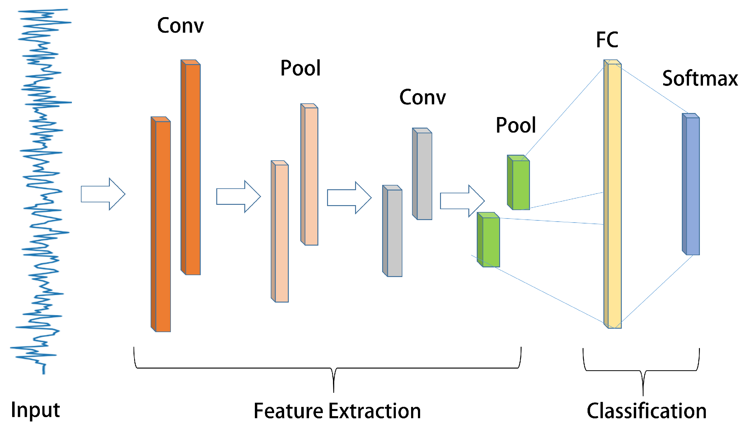
The typical structure of a CNN, as shown in Figure 2, consists of an input layer that is generally a grayscale image or a color image with three channels. Convolution and pooling layers, the fundamental components of a CNN structure, are responsible for constructing multiple filters that can extract features from the data. These layers convolve and pool the input data layer by layer, extracting the topological feature map concealed within the data. Sub-sampling can effectively utilize the local features inherent in the data’s characteristics, reducing data dimensionality, optimizing the network structure, and preventing overfitting. After passing through multiple convolutions and pooling layers, the pooled data are then expanded to a fully connected layer. This layer is connected to a hidden layer and ultimately mapped to the output layer using the softmax function.
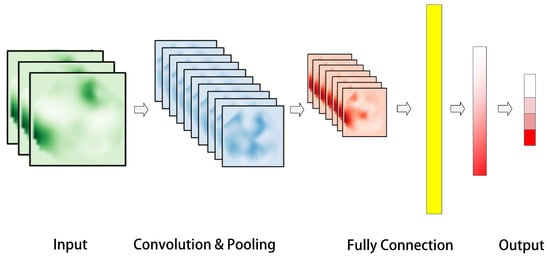
Figure 2.
Typical CNN structure.
3.2. 1D-CNN Model
Based on the basic structure depicted in Figure 3, 1D-CNN [27] is a convolutional neural network that utilizes one-dimensional convolution to extract features from one-dimensional time series while preserving temporal characteristics. In this study, the 1D-CNN structure is suitable for AUV fault diagnosis since the state signals consist of multiple 1D time series, meeting the input criteria of 1D-CNN.
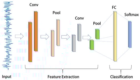
Figure 3.
The 1D-CNN structure.
The input to a one-dimensional convolution consists of one-dimensional data along with a one-dimensional convolution kernel. Similarly, the output of the corresponding convolution and pooling layer is also in a one-dimensional structure. The convolution operation can be denoted as follows:
where ∗ is the convolution operation; l is the l-th layer of the corresponding network; i and j denote the serial numbers of the feature maps in the l-th and -th layers, respectively; represents the feature map in the -th layer connected to the j-th feature map in the l-th layer; denotes the convolution kernel parameter; and is the bias.
To enhance the nonlinear approximation capability, convolutional operations are typically accompanied by activation functions, which modify the non-linear mapping of each convolutional output value. The commonly used nonlinear activation function is the rectified linear unit (ReLU), expressed as follows:
where is the output value of the convolution operation, and is the activation value of . The proposed nonlinear activation function mitigates the issue of overfitting by inducing some of the neuron outputs to be zero. This leads to increased sparsity in the network and diminishes the interdependence among the parameters.
The classification layer comprises a fully-connected implicit layer and a softmax layer, where the fully connected layer compresses the output of the previous pooling layer into a one-dimensional feature vector. Softmax, a generalization of logistic regression, addresses the multi-classification problem, with the number of output values equaling the number of label categories. Softmax achieves multi-classification by mapping the output of multiple neurons to the (0, 1) interval. Let us assume the category label and given a sample x; the probability of the sample x belonging to category k can be expressed as follows:
The measurement of the dissimilarity between the model output and the expected value necessitates the use of a loss function. In the case of the softmax regression model, the commonly employed loss function is the cross-entropy loss function, expressed as follows:
where and represent the raw data and labels of the training samples, respectively; N denotes the number of samples or the input batch size; k represents the number of categories; the indicator function is defined as 1 when the condition inside the brackets is true, and 0 otherwise; and corresponds to the model parameters of the training set, which are optimized to minimize the current cost function.
4. MC-FCNN-Based Fault Diagnosis
4.1. MC-FCNN Architecture
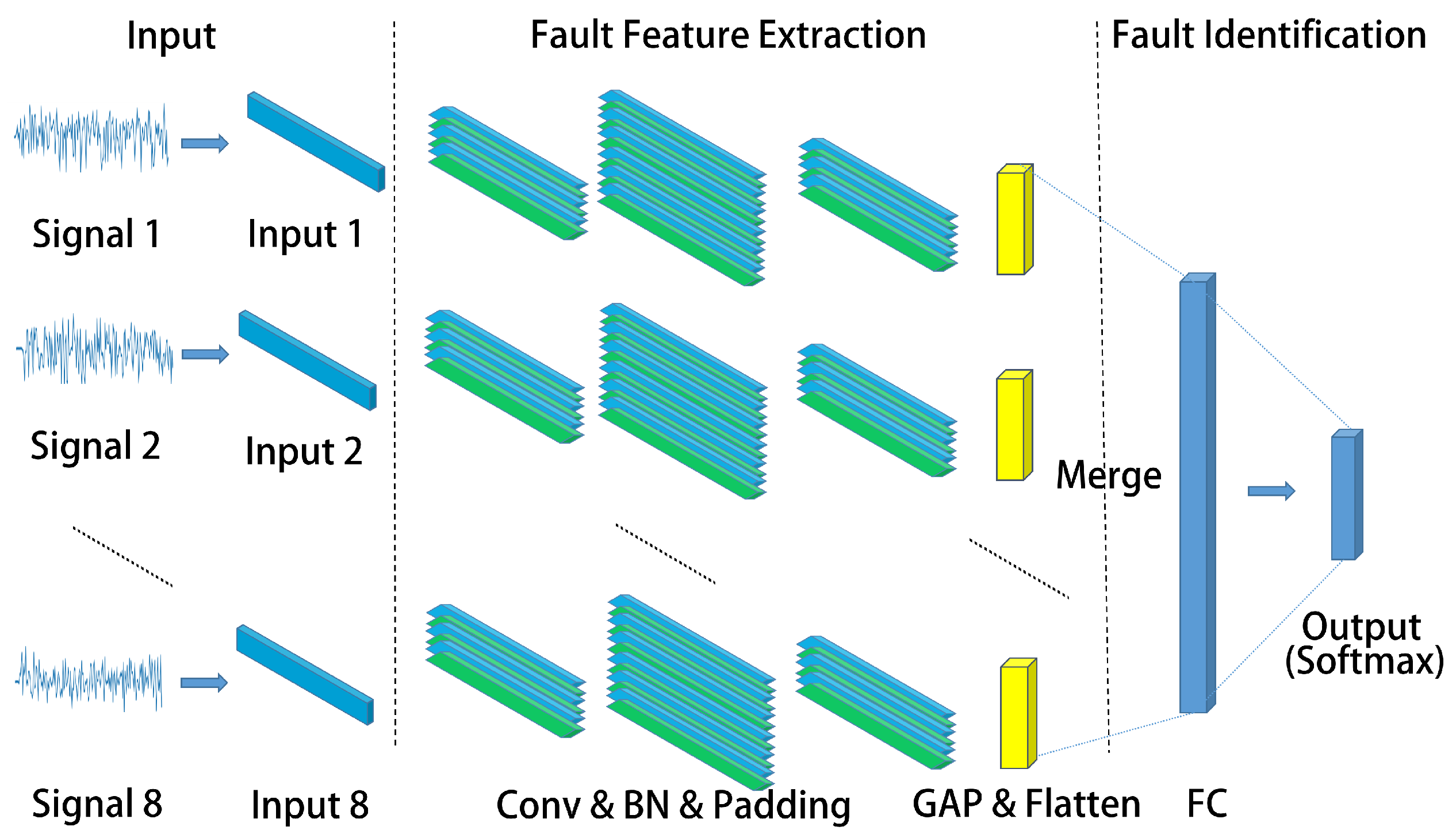
Unlike image data-based CNN inputs, the AUV state data consist of multiple one-dimensional time series, rather than two-dimensional image pixels. Therefore, the traditional 2D-CNN is improved in this paper by using the 1D-CNN as a feature extractor. This approach does not require complex transformation of the raw data, ensuring that temporal features are not lost. Taking into consideration that the AUV state is represented by multiple 1D time series data, we separate the multivariate time series into univariate time series. Building upon this, we designed a multi-channel strategy, where the number of channels corresponds to the number of sequences. The signal reflecting the state of AUV is composed of multiple sequence variables. There are typically two methods for fusing multi-sensor signals: data fusion and feature fusion. However, when fusing at the data end, it is easy to lose the unique characteristics of a single signal. To address this issue, we propose a multi-channel strategy. This strategy involves extracting and processing individual adaptive features of a single signal at the front end of the network and then fusing the signals at the feature end, which can increase the accuracy of fault diagnosis. In the case of AUV status signal, the number of channels is determined by the number of sensor signals. Moreover, our multi-channel strategy exhibits a certain level of generality, making it suitable for similar applications. Feature learning on the univariate series is performed separately and the traditional MLP is finally connected for classification. The FCNN has demonstrated outstanding performance in semantic [28]. It is capable of classifying images at the pixel level while retaining the spatial information of the input image. Drawing inspiration from this, we employ the FCNN as a feature extractor in our task to preserve the global information of the original subsequence. The architecture of the proposed MC-FCNN model is illustrated in Figure 4. The proposed fault diagnosis model based on MC-FCNN can be divided into three main components: signal pre-processing of AUV state data, feature extraction of fault state signals, and fault identification. The details of signal pre-processing for AUV state data will be discussed in Section 5.2. The input for MC-FCNN is denoted as , , where n represents the data dimension, l represents the sequence length, and represents 1D signal. Next, we will explain the process of feature extraction and fault identification.
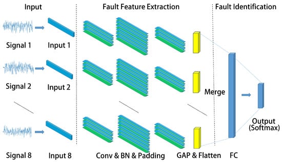
Figure 4.
MC-FCNN model.
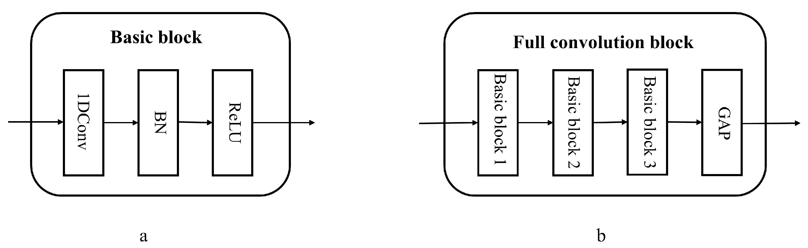
The fault feature extraction module consists of eight identical full convolution blocks running in parallel. Each full convolution block is composed of three basic blocks, namely 1D-Conv + BN (Batch Normalization) activated by ReLU, and global average pooling (GAP) [29]. Figure 5 shows the specific structures of the full convolution block and basic block, which can be represented as follows:
where ⊗ is the convolution operator. The GAP block takes the average value of the entire sequence feature map , where is the output of the previous basic block operation. The full convolution block is composed of three basic blocks and a GAP block. The convolution parameters for each basic block are illustrated in Table 1. The first basic block consists of 16 convolution kernels with a size of . The second basic block includes 32 convolution kernels with a size of , while the third basic block has 16 convolution kernels with a size of . The stride was set as 1, the padding was set to SAME, and the length of the vector remains unchanged before and after convolution. After each univariate signal passes through its corresponding feature extraction channel, the output feature map is obtained with a size of , where l represents the l-th feature extraction channel.
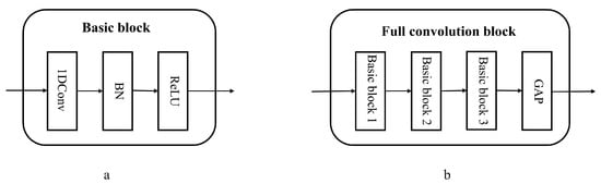
Figure 5.
(a) Basic block, (b) Full convolution block.

Table 1.
Full convolution block parameters.
The fault identification module is composed of two fully connected layers. The first fully connected layer performs the “flattening” operation on the features, where all feature maps are connected end-to-end to form a one-dimensional vector. The number of neurons in the second fully connected layer matches the number of fault categories. The softmax regression classifier is utilized to obtain the desired output category. The formula is as follows:
where is the output vector of the feature extraction layer, s is a -dimensional vector, is the number of fault categories. W and are the weights that need to be trained. In the softmax classifier, is a score of the i-th lable.
4.2. Fault Diagnosis Scheme
The flowchart of the MC-FCNN-based fault diagnosis scheme is illustrated in Figure 6, and the main steps are listed as follows:
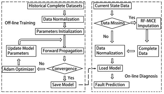
Figure 6.
MC-FCNN-based fault diagnosis scheme.
Step 1: Normalize a complete sample consisting of five types of sensor data using AUV normal states and four fault states as references.
Step 2: After parameter initialization, the normalized training data are taken as input for the MC-FCNN model. The error is calculated through forward propagation, and the parameters are then updated using model back-propagation.
Step 3: Finish training the model and save it along with the final parameters once the cross-entropy loss function converges.
Step 4: If online data are missing, normalize the imputed data using the random forest multiple imputation by chained equations algorithm.
Step 5: Load the trained model and use the processed data from step 4 as input. The resulting output from the current model will be the diagnosis result.
5. Experimental Results and Analysis
All experiments were conducted on a computer with the following specifications: Inter(R) Core(TM) i5-8300H CPU@2.30Ghz, 16 GB of RAM.
5.1. Experimental Data of AUVs
The AUV dataset used in this paper, which includes possible fault types, was derived from the Zhejiang University laboratory and can be accessed at https://data.mendeley.com/datasets/7rp2pmr6mx (accessed on 28 June 2021) [30]. The AUV dataset comprises a total of 1225 samples, consisting of normal working conditions and four fault conditions. The experimental prototype utilized is a quadrotor AUV named “Haizhe”, as depicted in Figure 7.
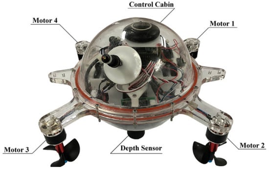
Figure 7.
Haizhe AUV [31].
The experimental dataset of the “Haizhe” AUV consists of five working conditions, representing possible fault types. These conditions are detailed in Table 2 and include load increase, normal, depth sensor failure, propeller severe damage, and propeller slight damage. Each fault type has been tested multiple times. During each test, the “Haizhe” AUV operates underwater for 10–20 s to ensure there is sufficient state data. Additionally, each sample in the dataset comprises 17 time series with constant lengths that reflect the current state of the “Haizhe” AUV, such as sensor signals, control signals, attitude signals, etc.
Table 2.
AUV working conditions.
5.2. Data Pre-Processing
Data pre-processing is crucial in CNN-based fault diagnosis, since the input data quality of the neural network has a direct influence on diagnosis accuracy. Except for this, due to the complexity of the deep-sea environment, a CNN-based AUV fault diagnosis scheme may not perform optimally when faced with missing data in certain working conditions. With these considerations in mind, this paper proposes a data pre-processing module that includes sequence length processing, feature dimension processing, data normalization, data missing design, and data imputation. In the following sections, each component of the data pre-processing module will be introduced in detail.
Sequence length processing: The sequence length is set to a fixed size. If the original sequence is not long enough, the last state data are used to fill the dataset. Conversely, if the sequence is longer than the desired length, the extra trailing data are removed. In the experimental dataset of this paper, the sequence length is specifically set to 196.
Feature dimension processing: In the provided dataset of the “Haizhe” AUV, each sample consists of 17 feature variables. It should be pointed out that, if all features are used, this will have a negative influence on the MC-FCNN-based fault diagnosis accuracy and the complexity of the model will increase at the same time. Therefore, this paper specifically selects eight feature variables, such as depth (), pressure (), roll (), pitch (), yaw (), angular velocity in roll (), angular velocity in pitch (), and angular velocity in yaw () for analysis and diagnosis.
Data normalization: Data normalization algorithms commonly used include max-min normalization, Z-score normalization, function transformation, and so on. In this study, considering the large volume of data in the raw dataset of the “Haizhe” AUV, Z-score normalization is chosen as the preferred method.
Data missing design and data imputation: To simulate the working conditions of the “Haizhe” AUV with data missing in the deep-sea environment, the missing rate of the raw dataset is set according to the following steps. Denote as the randomly missing feature variables in the raw dataset. The number of randomly missing values is denoted as , where r is the missing rate, n is the sequence length, and k is the number of missing variables. In the presence of working conditions with missing data, the RF-MICE technique introduced in the previous section is applied on the previous step of missing data design.
Remark: The data pre-processing for the “Haizhe” AUV is divided into two scenarios based on the integrity of the dataset. If the measurements are complete, the pre-processing module for the “Haizhe” AUV includes sequence length processing, feature dimension processing, and data normalization. However, in order to simulate working conditions with missing data, an extended pre-processing module is introduced, which comprises sequence length processing, feature dimension processing, data missing design, data imputation, and data normalization.
5.3. Comparisons
All the data from the “Haizhe” AUV working conditions, as shown in Table 2, are selected as the experimental samples. For each working condition, of the data is used for training, while the remaining is reserved for testing. The training algorithm employed is Adam with an initial learning rate of 0.001, and the objective function designed is to minimize the “cross-entropy”. In order to minimize the impact of randomness on the evaluation of data-driven fault diagnosis, 10 groups of training are implemented on the MC-FCNN model, with one group selected at random. The diagnosis results, as illustrated in Figure 8, demonstrate that the model proposed in this paper can effectively identify various “Haizhe” AUV working conditions.
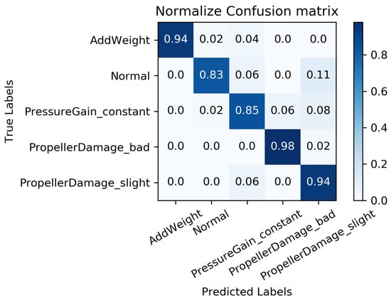
Figure 8.
Fault diagnosis results based on MC-FCNN.
Comparisons with three kinds of end-to-end fault diagnosis algorithms are presented in Figure 9 to validate the effectiveness of the model proposed in this paper, particularly in terms of diagnosis accuracy. The 1D-CNN network, as shown in Figure 2, consists of three convolutional pooling layers and two fully connected layers, with pre-processed data used as the input for the model. The fully convolutional networks (FCNs) proposed in the previous study [32] utilize three convolutional units and take pre-processed data as the model input. The residual network (ResNet) stacks three residual units with pre-processed data as the model input. Each model was trained using the same training set and algorithm, and the average accuracy of fault diagnosis was used as the comprehensive evaluation index on the same test set. Similarly, to mitigate the impact of randomness on diagnosis accuracy, 10 sets of training were performed on the diagnosis models to obtain average diagnosis results. Figure 10, Figure 11 and Figure 12 illustrate the diagnosis results of the three benchmark models.
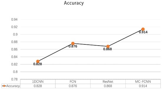
Figure 9.
Average accuracy comparisons between different neural network architectures.
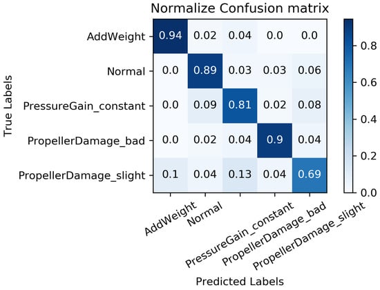
Figure 10.
Fault diagnosis results based on 1D-CNN.
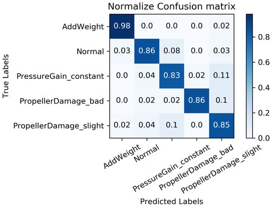
Figure 11.
Fault diagnosis results based on FCN.

Figure 12.
Fault diagnosis results based on ResNet.
The accuracy comparisons between different neural network architectures illustrated in Figure 10, Figure 11 and Figure 12 reveal that FCN achieves the highest accuracy of among the benchmark models including 1D-CNN, FCN, and ResNet. This suggests that the full convolutional network is a robust tool for processing features in sequence data. However, it is worth noting that the aforementioned benchmark models may overlook the distinctive features of individual sequences as they directly extract fused features from multi-sensor data. To address this issue, the proposed fault diagnosis model based on the MC-FCNN incorporates feature extraction and fusion techniques with multiple channel inputs, resulting in an impressive accuracy of 91.4%. This outcome highlights the superiority of the proposed multi-channel strategy for handling multi-sensor sequence data. Furthermore, the analysis conducted on the “Haizhe” AUV state data can also be utilized for potential fault predictions.
5.4. MC-FCNN-Based Fault Diagnosis Analysis with Different Missing Data
According to the analysis in the previous sections, the MC-FCNN-based AUV fault diagnosis scheme cannot achieve ideal performance when sensor signals are absent due to the complexity of the deep-sea environment, since neural network inputs with missing data will result in inaccurate diagnosis results. In this section, the RF-MICE algorithm proposed in Section 2 will be combined to impute the online missing data, and then the MC-FCNN model trained in Section 5.3 will be used for fault classification verification. The data used for testing in the experiments are the same as the test dataset in Section 5.3. Each sample comprises eight feature variables: , , , , , , , and , where , and are assumed as missing variables with the pattern of missing at random (MAR).
5.4.1. Evaluation of Missing Data Imputation Based on RF-MICE
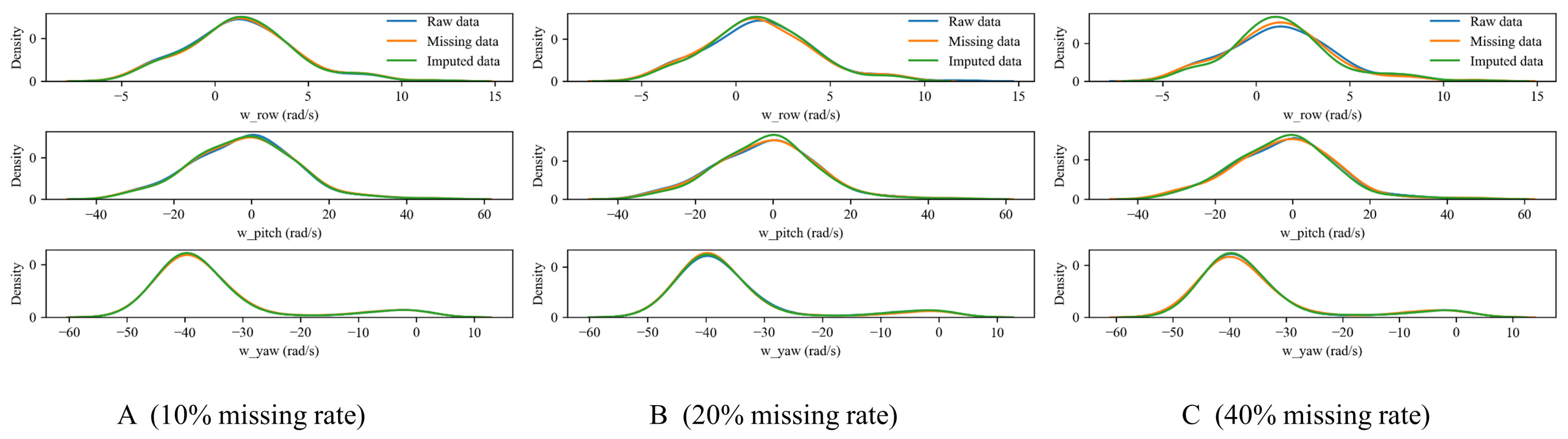
Denote the missing rate , where N is the total number of missing values, n is the variable length, and k is the number of missing variables. We aim to analyze the imputation performance of the proposed RF-MICE method when the missing rate in each sample data is , and , where . Our data imputation module is designed to be dynamic, rather than a fixed model trained solely on historical data. When encountering an online sample for diagnosis with missing data, the imputation function is triggered. In this case, our imputation model is trained by using the available data from the online sample, and the missing values are predicted and imputed. As a result, a complete data sample is generated and serves as the input for the fault diagnosis model. The imputation algorithm proposed in this paper retrains every missing sample to restore its real distribution to the greatest extent possible. The RF-MICE algorithm requires setting the iteration parameter “iter” and the parallel parameter “m”. In our experiment, we set iter = 3 and m = 4. Figure 13 displays the actual probability density distribution curve for each missing variable and the probability density distribution curve after imputation.
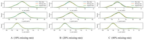
Figure 13.
Theprobability distribution comparisons between raw data, missing, data and imputed data.
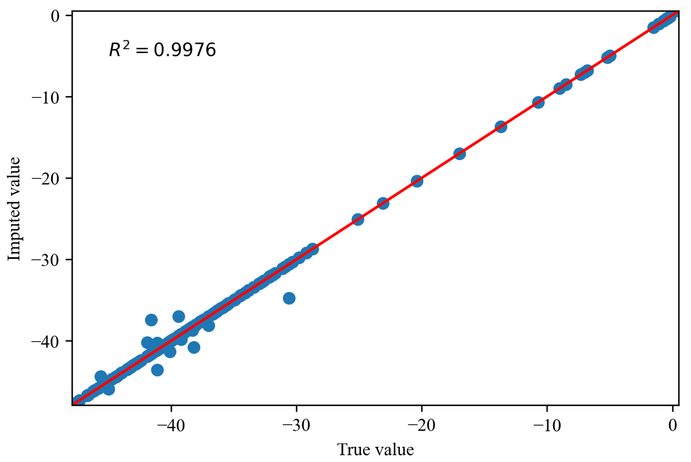
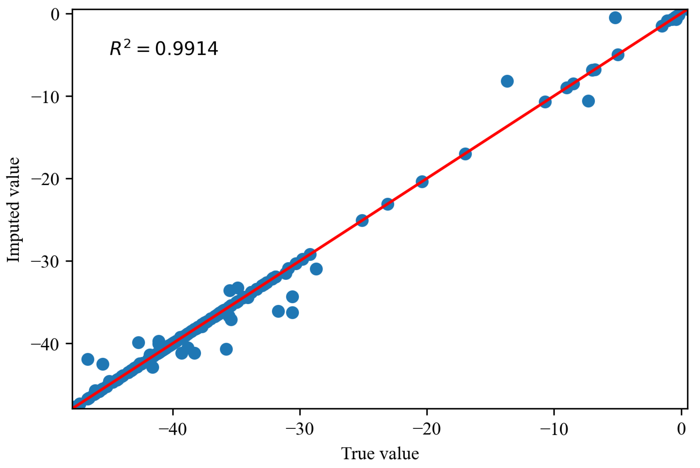
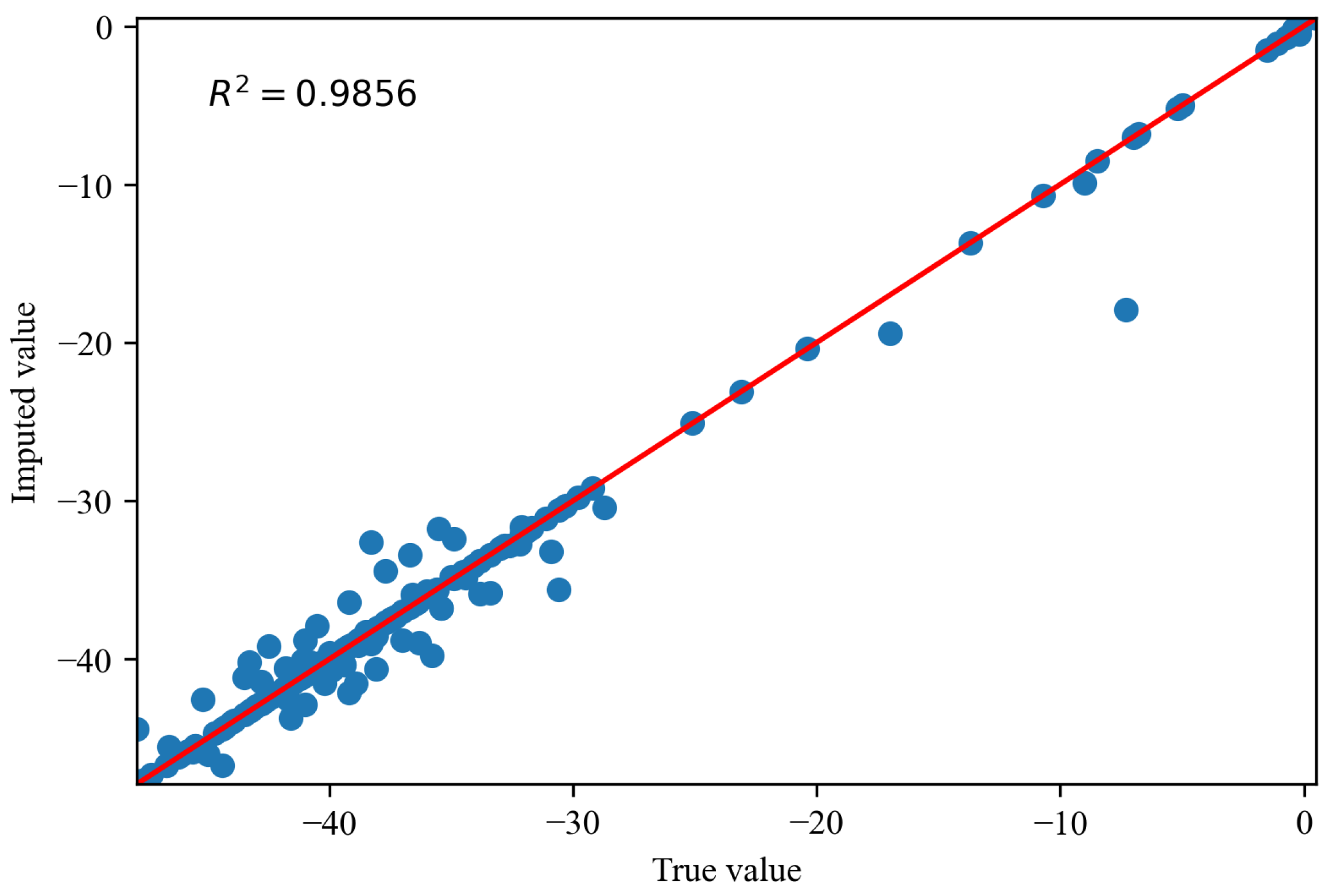
Figure 14, Figure 15 and Figure 16 depict the comparisons between the actual values and imputed values of the randomly selected missing variable , with the representation of R squared () indicating the accuracy of data imputation. By comparing Figure 13, we can find that, as the missing degree increases, the deviation in distribution between the imputed values of the variable and the original data gradually increases. On the other hand, there is no noticeable difference in the distribution deviation between the imputed values of the variables and with the original data. It is noteworthy that, regardless of the degree of missing values, our proposed imputation method yields imputed distributions that closely resemble the original distribution. This suggests that our imputation method does not alter the distribution of the original data. By comparing Figure 14, Figure 15 and Figure 16, we can find gradual decreases in the values of as the degree of missing data increases. However, the decreases are not statistically significant. In addition, the values of are consistently close to 1, signifying the excellent performance of our imputation method.
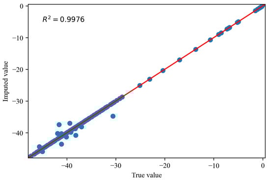
Figure 14.
Thecomparisons of the actual values and imputed values when missing rate is .
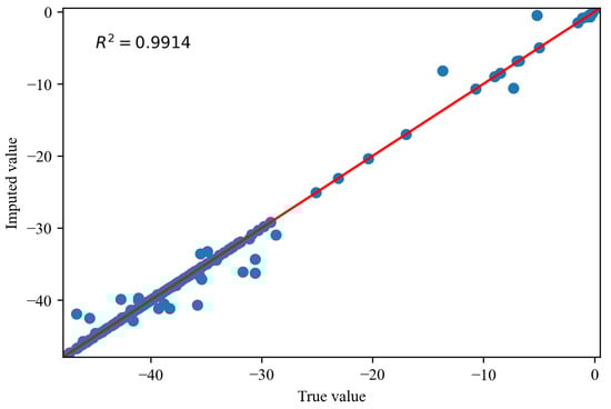
Figure 15.
The comparisons of the actual values and imputed values when missing rate is .

Figure 16.
The comparisons of the actual values and imputed values when missing rate is .
5.4.2. Fault Diagnosis Result with Different Missing Data
The primary objective of the experiment is to analyze the impact of our trained MC-FCNN model on the diagnosis results. This analysis will be performed when all of the data have been imputed using our proposed RF-MICE method. The experiment will be conducted with different data missing rates; specifically, missing rates of , , , , and .
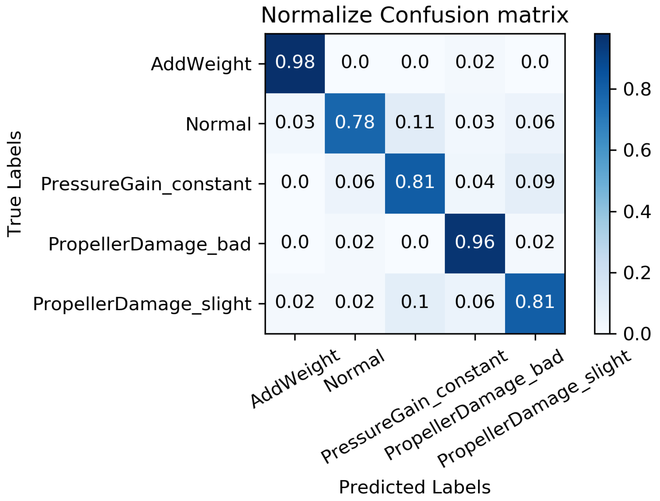
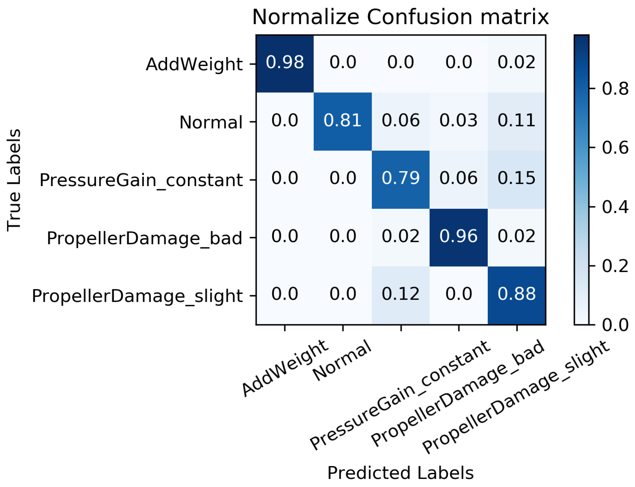
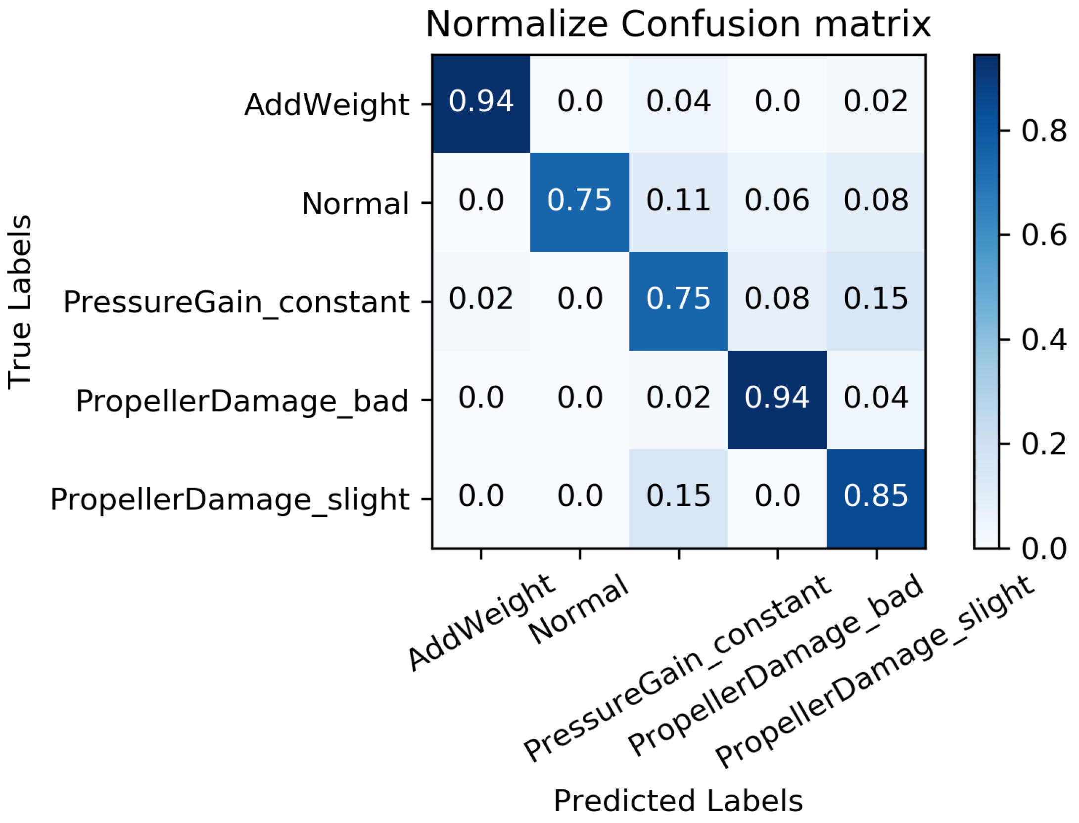
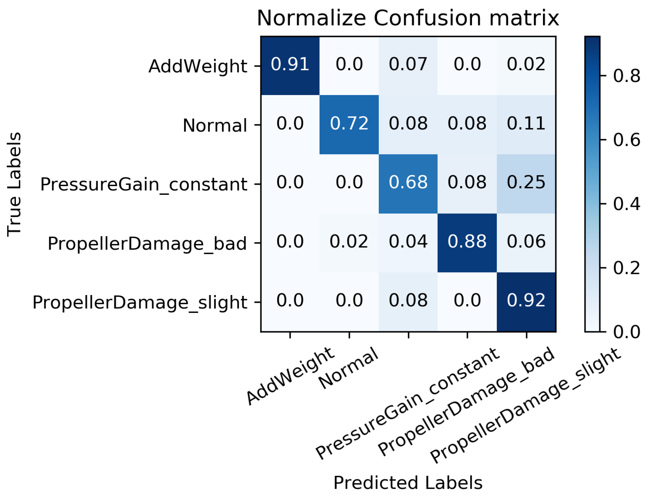
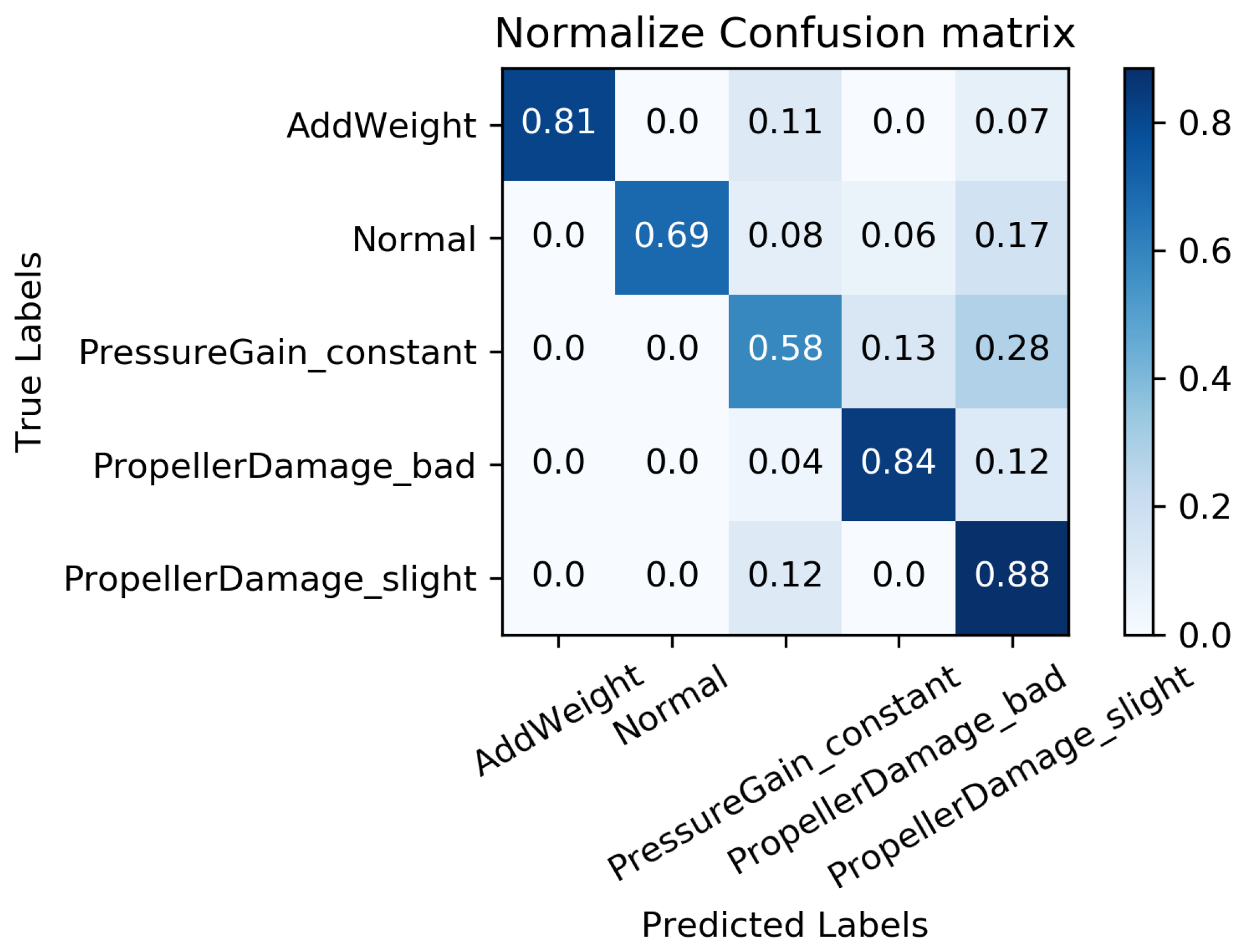
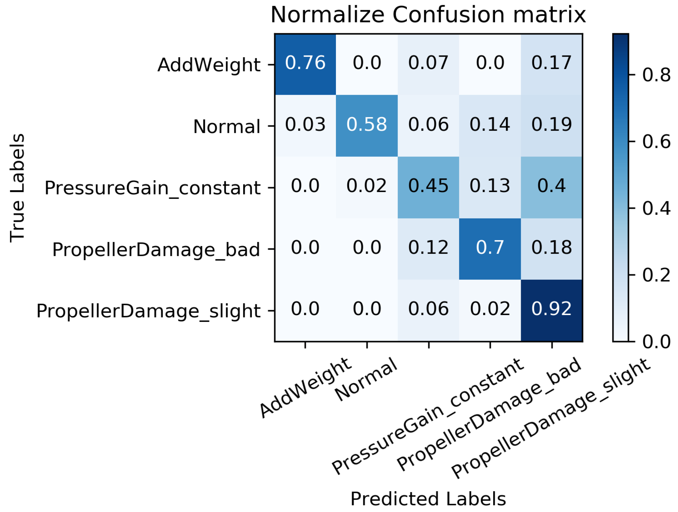
We constructed a confusion matrix, as shown in Figure 17, Figure 18, Figure 19, Figure 20 and Figure 21, to analyze the diagnosis results of the MC-FCNN model under different missing data scenarios. The confusion matrix provides an intuitive reflection of the model’s classification performance on different fault categories. It presents the correspondence between the predicted results of the classifier and the actual fault categories. The vertical axis represents the real fault categories, while the horizontal axis represents the model’s predicted results for each category. Interestingly, by comparing Figure 17, Figure 18, Figure 19, Figure 20 and Figure 21, it is evident that, with varying degrees of data loss, fault types or working conditions such as load increase, normal, depth sensor failure, and propeller severe damage are predominantly misdiagnosed as propeller slight damage. However, propeller slight damage is frequently misdiagnosed as normal working condition. This pattern suggests that propeller slight damage, being an incipient fault, may have a significant impact on the diagnosis of other fault types.

Figure 17.
Fault diagnosis results when missing rate is .
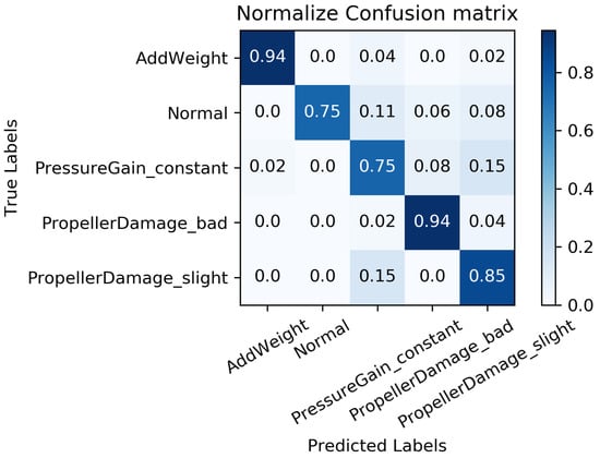
Figure 18.
Fault diagnosis results when missing rate is .

Figure 19.
Fault diagnosis results when missing rate is .

Figure 20.
Fault diagnosis results when missing rate is .
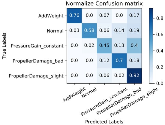
Figure 21.
Fault diagnosis results when missing rate is .
In order to evaluate the overall diagnostic performance of the model under different missing data scenarios, we combined the fault diagnosis results of the MC-FCNN model with the RF-MICE technique. The analysis, as shown in Table 3, includes missing rates ranging from 10% to 80%. The working conditions 0–4 correspond to the AUV working conditions mentioned in Table 2, which include load increase, normal, depth sensor failure, propeller severe damage, and propeller slight damage.
Table 3.
MC-FCNN-based fault diagnosis with different missing rates.
As expected, the overall diagnostic accuracy of our model declined as the degree of missingness increased. However, it is worth noting that our model maintained an ideal diagnostic performance even with a data missing rate as high as 60%. Upon further analysis, we observed that different missing data rates had a significant impact on the diagnostic performance of working conditions 1 and 2 (normal and depth sensor failure). This can be attributed to the fact that attitude–velocity signals play a crucial role in identifying normal working conditions and depth sensor failures, and their absence can lead to a severe misdiagnosis of these two states.
6. Conclusions
In this paper, we propose a model-free AUV fault diagnosis scheme based on the MC-FCNN and RF-MICE technique for handling missing data. The deep learning-based fault diagnosis model makes several contributions: (1) It utilizes a multi-channel input strategy to extract unique features from each signal, enabling the processing of multi-sensor time series data; (2) By leveraging the end-to-end feature of deep learning, the model can learn the patterns between AUV states and possible fault types, leading to a simplified diagnosis process through integrated fault detection and isolation; (3) To address potential data loss in online scenarios, we propose the RF-MICE algorithm, which combines the MC-FCNN model for online diagnosis. Our future work will focus on enhancing the generalization capability of the convolutional neural network-based fault diagnosis model, particularly when addressing unknown types of faults that are beyond the scope of the training set.
Author Contributions
Conceptualization: Y.W. and A.W.; methodology: A.W. and Y.Z.; software: A.W.; validation: Y.W. and A.W.; formal analysis: Y.W.; investigation: A.W.; resources: Q.Z.; data curation: Q.Z. and A.W.; writing—original draft preparation: A.W.; writing—review and editing: Y.W.; visualization: Z.Z.; supervision: Z.Z.; project administration: Y.W.; funding acquisition: Y.W. All authors have read and agreed to the published version of the manuscript.
Funding
This work was supported in part by the National Natural Science Foundation of China under Grants (62173164, 62203192), in part by the Natural Science Foundation of Jiangsu Province of China under Grant BK20201451, in part by the 6th regular meeting exchange program (6-3) of China-North Macedonian science and technology cooperation committee.
Conflicts of Interest
The authors declare no conflict of interest.
Abbreviations
The following abbreviations are used in this manuscript:
| MLP | Multilayer Perception |
| MC-FCNN | Multi Channel Full Convolutional Neural Network |
| AUV | Autonomous Underwater Vehicle |
| RF-MICE | Random Forest Multiple Imputation by Chained Equations |
| MAR | Missing At Random |
References
- Freeman, P.; Pandita, R.; Srivastava, N.; Balas, G.J. Model-based and data-driven fault detection performance for a small UAV. IEEE ASME Trans. Mechatron. 2013, 18, 1300–1309. [Google Scholar] [CrossRef]
- Chen, H.T.; Liu, Z.G.; Alippi, C.; Huang, B.; Liu, D. Explainable intelligent fault diagnosis for nonlinear dynamic systems: From unsupervised to supervised learning. IEEE Trans. Neural Netw. Learn. 2022, 8, 1–14. [Google Scholar] [CrossRef] [PubMed]
- Chen, H.T.; Luo, H.; Huang, B.; Jiang, B.; Kaynak, O. Transfer Learning-Motivated Intelligent Fault Diagnosis Designs: A Survey, Insights, and Perspectives. IEEE Trans. Neural Netw. Learn. 2023, 7, 1–15. [Google Scholar] [CrossRef] [PubMed]
- Abed, W.; Sharma, S.; Sutton, R. Neural network fault diagnosis of a trolling motor based on feature reduction techniques for an unmanned surface vehicle. Proc. Inst. Mech. Eng. H 2015, 229, 738–750. [Google Scholar] [CrossRef]
- Zhang, M.J.; Yin, B.J.; Liu, W.X.; Wang, Y.J. Fault feature extraction and fusion of AUV thruster under random interference. J. Huazhong Univ. Sci. Technol. 2015, 43, 22–54. [Google Scholar]
- Chauhan, V.K.; Dahiya, K.; Sharma, A. Problem formulations and solvers in linear SVM: A review. Artif. Intell. Rev. 2019, 52, 803–855. [Google Scholar] [CrossRef]
- Zhang, M.J.; Wu, J.; Chu, Z. Multi-fault diagnosis for autonomous underwater vehicle based on fuzzy weighted support vector domain description. China Ocean Eng. 2014, 28, 599–616. [Google Scholar] [CrossRef]
- Zhao, R.; Yan, R.Q.; Chen, Z.H.; Mao, K.Z.; Wang, P.; Gao, R.X. Deep learning and its applications to machine health monitoring. Mech. Syst. Signal Process. 2019, 115, 213–237. [Google Scholar] [CrossRef]
- Lei, Y.G.; Yang, B.; Jiang, X.W.; Jia, F.; Li, N.P.; Nandi, A.K. Applications of machine learning to machine fault diagnosis: A review and roadmap. Mech. Syst. Signal Process. 2020, 138, 106587. [Google Scholar] [CrossRef]
- Tang, S.N.; Yuan, S.Q.; Zhu, Y. Deep learning-based intelligent fault diagnosis methods toward rotating machinery. IEEE Access 2019, 8, 9335–9346. [Google Scholar] [CrossRef]
- Zhu, D.Q.; Sun, B. Information fusion fault diagnosis method for unmanned underwater vehicle thrusters. IET Electr. Syst. Transp. 2013, 3, 102–111. [Google Scholar] [CrossRef]
- Nascimento, S.; Valdenegro-Toro, M. Modeling and soft-fault diagnosis of underwater thrusters with recurrent neural networks. IFAC-PapersOnLine 2018, 51, 80–85. [Google Scholar] [CrossRef]
- Ren, H.; Qu, J.F.; Chai, Y.; Tang, Q.; Ye, X. Deep learning for fault diagnosis: The state of the art and challenge. J. Control Decis. 2017, 32, 1345–1358. [Google Scholar]
- Jiang, Y.; Feng, C.; He, B.; Guo, J.; Wang, D.R.; PengFei, L.V. Actuator fault diagnosis in autonomous underwater vehicle based on neural network. Sens. Actuators A 2021, 324, 112668. [Google Scholar] [CrossRef]
- Yeo, S.J.; Choi, W.S.; Hong, S.Y.; Song, J.H. Enhanced convolutional neural network for in Situ AUV thruster health monitoring using acoustic signals. Sensors 2022, 22, 7073. [Google Scholar] [CrossRef] [PubMed]
- Chen, Y.M.; Wang, Y.Z.; Yu, Y.; Wang, J.R.; Gao, J. A Fault Diagnosis Method for the Autonomous Underwater Vehicle via Meta-Self-Attention Multi-Scale CNN. J. Mar. Sci. Eng. 2023, 11, 1121. [Google Scholar] [CrossRef]
- Ji, D.X.; Yao, X.; Li, S.; Tang, Y.G.; Tian, Y. Model-free fault diagnosis for autonomous underwater vehicles using sequence convolutional neural network. Ocean Eng. 2021, 232, 108874. [Google Scholar] [CrossRef]
- Jinn, J.H.; Sedransk, J. Effect on secondary data analysis of common imputation methods. Sociol. Methodol. 1989, 19, 213–241. [Google Scholar] [CrossRef]
- Khatibisepehr, S.; Huang, B. Dealing with Irregular Data in Soft Sensors: Bayesian Method and Comparative Study. Ind. Eng. Chem. Res. 2008, 47, 8713–8723. [Google Scholar] [CrossRef]
- Thomas, T.; Rajabi, E. A systematic review of machine learning-based missing value imputation techniques. Data Technol. Appl. 2021, 55, 558–585. [Google Scholar] [CrossRef]
- Kokla, M.; Virtanen, J.; Kolehmainen, M.; Paananen, J.; Hanhineva, K. Random forest-based imputation outperforms other methods for imputing LC-MS metabolomics data: A comparative study. BMC Bioinf. 2019, 20, 1–11. [Google Scholar] [CrossRef] [PubMed]
- Feng, R.; Grana, D.; Balling, N. Imputation of missing well log data by random forest and its uncertainty analysis. Comput. Geosci. 2021, 152, 104763. [Google Scholar] [CrossRef]
- Van, B.S.; Groothuis, O.K. mice: Multivariate imputation by chained equations in R. J. Stat. Softw. 2011, 45, 1–67. [Google Scholar]
- Breiman, L. Random forests. Mach. Learn. 2001, 45, 5–32. [Google Scholar] [CrossRef]
- Azur, M.J.; Stuart, E.A.; Frangakis, C.; Leaf, P.J. Multiple imputation by chained equations: What is it and how does it work? Int. J. Methods Psychiatr. Res. 2011, 20, 40–49. [Google Scholar] [CrossRef] [PubMed]
- Gu, J.X.; Wang, Z.H.; Kuen, J.; Ma, L.Y.; Shahroudy, A.; Shuai, B.; Liu, T.; Wang, X.X.; Wang, G.; Cai, J.F. Recent advances in convolutional neural networks. Pattern Recognit. 2018, 77, 354–377. [Google Scholar] [CrossRef]
- Kiranyaz, S.; Avci, O.; Abdeljaber, O.; Ince, T.; Gabbouj, M.; Inman, D.J. 1D convolutional neural networks and applications: A survey. Mech. Syst. Signal Process. 2021, 151, 107398. [Google Scholar] [CrossRef]
- Long, J.; Shelhamer, E.; Darrell, T. Fully convolutional networks for semantic segmentation. In Proceedings of the IEEE Conference on Computer Vision and Pattern Recognition (CVPR), Boston, MA, USA, 11–12 June 2015; pp. 3431–3440. [Google Scholar]
- Lin, M.; Chen, Q.; Yan, S. Network In Network. arXiv 2013, arXiv:1312.4400. [Google Scholar]
- Ji, D.X.; Yao, X.; Li, S.; Tang, Y.G.; Tian, Y. Autonomous underwater vehicle fault diagnosis dataset. Data Brief. 2021, 39, 107477. [Google Scholar] [CrossRef]
- Ji, D.X.; Wang, R.; Zhai, Y.Y.; Gu, H.T. Dynamic modeling of quadrotor AUV using a novel CFD simulation. Ocean Eng. 2021, 237, 1096501. [Google Scholar] [CrossRef]
- Wang, Z.; Yan, W.; Oates, T. Time series classification from scratch with deep neural networks: A strong baseline. In Proceedings of the 2017 International Joint Conference on Neural Networks (IJCNN), Anchorage, AK, USA, 14–19 May 2017; pp. 1578–1585. [Google Scholar]


Disclaimer/Publisher’s Note: The statements, opinions and data contained in all publications are solely those of the individual author(s) and contributor(s) and not of MDPI and/or the editor(s). MDPI and/or the editor(s) disclaim responsibility for any injury to people or property resulting from any ideas, methods, instructions or products referred to in the content. |
© 2023 by the authors. Licensee MDPI, Basel, Switzerland. This article is an open access article distributed under the terms and conditions of the Creative Commons Attribution (CC BY) license (https://creativecommons.org/licenses/by/4.0/).