Article

Identification of Tool Wear Based on Infographics and a Double-Attention Network

School of Mechanical Engineering, Hangzhou Dianzi University, Hangzhou 310018, China
*
Author to whom correspondence should be addressed.
Machines 2023, 11(10), 927; https://doi.org/10.3390/machines11100927
Submission received: 30 August 2023 / Revised: 20 September 2023 / Accepted: 24 September 2023 / Published: 26 September 2023
(This article belongs to the Section Friction and Tribology)

Abstract

:
Tool wear is a crucial factor in machining as it directly impacts surface quality and indirectly decreases machining efficiency, which leads to significant economic losses. Hence, monitoring tool wear state is of the utmost importance for achieving high performance and efficient machining. Although monitoring tool wear state using a single sensor has been validated in laboratory settings, it has certain drawbacks such as limited feature information acquisition and inability to learn important features adaptively. These limitations pose challenges to quickly extending the monitoring function of tool wear state of the machine tools. To solve these problems, this paper proposes a double-attention deep learning network based on vibroacoustic signal fusion feature infographics. The first solution is the construction of novel infographics using tool-intrinsic characteristics and multi-domain fusion features of multi-sensor inputs, which includes correlation analysis, principal component analysis, and feature fusion. The second solution is to build a novel deep network with a double-attention module and a spatial pyramid pooling module which can accurately and quickly identify tool wear state by successfully extracting critical spatial data from the infographics at various scales. The validity of the network is examined through an interpretability analysis based on the class activation graph. In terms of the tool wear status recognition task, the F1 score of the double-attention model based on an information graph is 11.61% higher than Resnet18, and peak recognition accuracy reaches 97.98%.

1. Introduction

Precise high-end machining centers play a critical role in high-performance manufacturing due to their ability to carry out complex and diverse processes [1]. In the realm of high-performance machining and manufacturing, the tool serves as the direct executor of the machining process and is prone to chemical wear, physical wear, and various abnormal states, all of which directly impact the surface quality, machining accuracy, and overall lifespan of the workpiece [2]. Consequently, the state of the tool significantly influences the quality of the workpiece during the machining process. According to statistics from the period between 2000 and 2010, approximately 20% of machine tool shutdowns can be attributed to tool failures, resulting in actual service lives that range from 50% to 80% of the recommended service life [3,4]. Although the data are relatively outdated, annual economic loss directly or indirectly caused by tool failure is still very large. Therefore, tool wear monitoring technology has garnered extensive attention from industrial engineers and scientific researchers. Monitoring the state of tool wear holds enormous significance for maintaining cutting performance and ensuring the surface quality of the workpiece, thereby mitigating adverse effects caused by worn-out tools on both the workpiece and the processing equipment [5].
Monitoring tool wear state involves two primary steps: collecting the data generated during the tool wear process and building a model based on this data to predict tool wear state. According to the type of data collected, they can be divided into direct method and indirect method. In the direct method, an image of the worn tool is captured using a CCD camera and a lighting unit. The information within the image is then utilized to predict the tool wear state. Kerr et al. [6] used digital image-processing technology to analyze the wear image of the tool and complete the evaluation of the tool wear state. Kassim et al. [7] utilized tool surface texture to indicate wear status and conducted tool status monitoring using machine vision techniques including image enhancement and segmentation. The field of tool wear state monitoring has seen extensive application of computer vision technology due to advancements in information technology. Zhou et al. [8] successfully detected tool wear state on-site by applying computer vision technology based on deep learning, significantly enhancing detection efficiency.
The direct method offers a significant advantage due to its versatility in addressing various machine tools and cutting conditions, enabling precise outcomes through the implementation of machine vision and computer vision technologies. Nonetheless, challenges emerge from issues such as the splashing of cutting fluid during machining and the spatial orientation of the tool on the workpiece, which hinder the acquisition of tool images. Moreover, avoiding the uneven distribution of light on a curved tool’s surface when capturing images poses a challenge. As a result, the demanding processing environment, the constrained and intricate spatial relationship between the tool and the workpiece, and the lighting intricacies during image capture confine direct measurement technology primarily to laboratory settings, with limited applicability in industrial contexts.
The indirect approach involves monitoring signals during the cutting process, including cutting force, acoustic emission, and current, among others, to forecast the tool’s condition. Silva et al. [9] believed that cutting force becomes highly responsive to friction after tool wear, rendering it the most dependable technique for prognosticating the tool’s wear state through the utilization of cutting force data obtained from the dynamometer. The gradual deterioration of the tool is intricately linked to the material’s brittle fracture and plastic deformation. Wang et al. [10] leveraged the clustering energy of the AE burst signal as a means to decide the wear state of the tool flank. Loenzo et al. [11] comprehensively investigated cutting tool lifecycle from initial use to failure, subsequently discovering the capacity of cumulative cutting power to accurately pinpoint the tool’s fractured condition. Despite the capability of these indirect measurement technologies to monitor tool wear state, practical application is significantly curtailed by the intricate and personalized sensor installation and fixation procedures, coupled with their substantial cost.
Sensors for acoustic and vibration signals have attracted the attention of researchers due to their affordability and ease of installation. Li et al. [12] employed Fast Fourier Transform (FFT) and a band-pass filter to eliminate acoustic signal noise during the cutting process. Subsequently, they applied the Blind Source Separation (BSS) algorithm for denoising. Following initial signal preprocessing, Short-Time Fourier Transform (STFT), Power Coherence Transform (PCT), and Wigner–Ville Distribution (WVD) were employed to individually convert the audio signal into spectrogram images. The identification of tool wear state was conducted by integrating three sub-Convolutional Neural Network (CNN) models. Zhou et al. [13] monitored tool wear acoustics using a two-layer angular kernel Extreme Learning Machine (ELM), utilizing a subset of acoustic sensor parameters for wear condition identification. Prakash and Samraj [14] applied Singular Value Decomposition (SVD) to analyze acoustic signals for tool wear monitoring in close-gap turning. Vibration, akin to cutting force, also exhibits strong sensitivity to tool conditions. Shi et al. [15] achieved tool wear prediction by extracting multi-dimensional features from distinct feature domains in the original vibration signal. Twardowski et al. [16] predicted tool wear in cast iron milling through various machine learning classification tree forms using vibration signals. Bahador et al. [17] introduced tool wear detection in the turning process utilizing a one-dimension neural network and transfer learning. Wang et al. [18] transformed vibration sensor data into images, serving as inputs for CNN models to monitor mechanical fault conditions in the manufacturing industry. Whether relying on acoustic or vibration signals or not, individual sensors often provide incomplete signal information due to inherent limitations and environmental interference.
The method of multi-sensor fusion monitoring harnesses the synergistic advantages of multiple sensor signals, thereby improving anti-interference capabilities and ensuring a more comprehensive monitoring signal. This establishes a robust correlation with tool wear [19]. Rafezi et al. [20] monitored tool wear utilizing both acoustic and vibration signals in tandem with Wavelet Packet Decomposition (WPD). Similarly, Gomes et al. [21] employed Support Vector Machines (SVM) to analyze vibration and sound signals, subsequently leveraging Recursive Feature Elimination (RFE) to discern the most pertinent features for tool wear during micro milling. Not all features from multi-source signals are relevant to the model, underscoring the significance of feature selection strategy. Niaki et al. [22] implemented Principal Component Analysis (PCA) to categorize monitoring features, thus eliminating superfluous and irrelevant data to bolster monitoring accuracy. Meanwhile, Niu et al. [23] extracted features from time, frequency, and time-frequency domains, utilizing an information measure-based feature selection method to reduce dimensionality, selecting those features strongly correlated with tool wear. However, the above feature selection strategy does not consider the relevant information about the tool itself. In addition, the importance of features cannot be adaptively adjusted according to changes in features. However, the attention module in deep learning can selectively highlight those more discriminative features. Moreover, the pyramid convolution-pooling module can collect and fuse features at multiple scales. Therefore, this research endeavors to amalgamate multi-sensor features with intrinsic tool characteristics to craft a vibroacoustic signal fusion feature infographic for the cutting process. Employing deep learning techniques, a convolutional neural network is devised to discern the condition of a worn tool using this infographic.
In this study, we initially process the features of multi-sensor signals across multiple domains. The selected features are those acutely sensitive to and strongly correlated with tool wear. These salient features are fused using Principal Component Analysis (PCA). An infographic based on fused features and the cut times is constructed. The fused feature map contains feature information that is highly related to tool wear and the intrinsic information of the tool. Then, we introduce a double-attention pyramid convolutional network model, devised to adaptively discern features within infographics crucial for tool wear state identification. The dual-attention module adeptly extracts spatial features and judiciously allocates them. To mitigate challenges like vanishing gradients in deep networks, our model employs residual blocks. Additionally, the spatial pyramid convolution-pooling module captures pertinent information across various scales within the network. Hence, this research leverages machine learning and computer vision methodologies to identify tool wear state. The fusion of multi-sensor signal features into an infographic, in tandem with the double-attention pyramid convolutional network model, is helpful in elevating the precision and accuracy of tool wear state identification.
The paper is structured as follows: Section 2.1 details the creation of the vibroacoustic signal fusion feature infographic. Section 2.2 presents the fundamental theory of the network architecture, followed by descriptions of its constituent modules. Section 2.3 outlines the tool wear state identification methodology. Section 3.1 describes the experimental setup and data collection process. Section 3.2 focuses on the measurement of flank wear VB during experiments. Section 3.3 discusses data preprocessing and the utilization of the dataset for model training and validation. In Section 4.1, we compare the training and performance of various models. Section 4.2 delves into model interpretability. Finally, conclusions and prospects are addressed in Section 5.

2. Theoretical Framework

2.1. Vibroacoustic Signal Feature Fusion Infographic

Initially, the truncated vibroacoustic signal undergoes feature extraction in the time domain, frequency domain, and time-frequency domain. In the time domain, 17 features are extracted, including mean, standard deviation, skewness, kurtosis, peak-to-peak value, RMS value, crest factor, form factor, pulse factor, margin factor, kurtosis factor, absolute value mean, the maximum value, variance, square root magnitude, peak value, minimum value and maximum value. Following a Fast Fourier Transform (FFT) on the time-domain signal, features such as average amplitude, center of gravity frequency, mean square frequency, variance frequency, and frequency variance of the spectrum are derived. Additionally, from the power spectrum, we extract the average frequency, median frequency, total power, average power, maximum power and low frequency to high frequency power ratio resulting in 11 frequency domain features in total. For the time-frequency domain, the db6 wavelet decomposes the signal into a three-layer wavelet packet. Features like wavelet energy entropy, wavelet singular entropy, wavelet energy ratio of each sub-band, and sub-band wavelet entropy are obtained, totaling 18 time-frequency domain features. According to Table A1, Table A2 and Table A3, the features of the signal in the time domain, frequency domain, and time-frequency domain are extracted. A correlation analysis is subsequently conducted between these diverse domain features and the tool wear value VB. Figure 1a is the visualization of the correlation coefficient matrix between the three domain features and the tool wear VB. The correlation calculation formula is as follows [24]:
ρ X , Y = cov ( X , Y ) σ X σ Y = E ( ( X μ X ) ( Y μ Y ) ) σ X σ Y
where μ X and μ Y denote the mean of the feature and the wear value, respectively. σ X and σ Y denote the standard deviations of the feature X and the wear value Y , respectively. The features with the absolute value of the correlation coefficient greater than 0.5 are screened out, and the feature matrix highly correlated with the tool wear value is established.
Subsequently, to mitigate noise interference in signal features and enhance the generalizability of the model, Principal Component Analysis (PCA) [25] is employed on the matrix of highly correlated features. This process serves to fuse these features through dimensionality reduction. The steps for this PCA-based feature fusion are detailed below:
Step 1: normalize each column feature of the highly correlated feature matrix.
x * = x x min x x max
where x denotes features that have been screened for Pearson-related operations, and x * denotes normalized value. x min and x max denote the minimum and maximum value of x .
Step 2: obtain a highly correlated principal component feature matrix.
C u i = λ i u i
α i = k = 0 i λ k j = 1 n λ j , λ i λ i - 1 0
M = U T X
where C denotes the covariance matrix corresponding to the highly correlated feature matrix, then λ i and u i denote corresponding eigenvalues and eigenvectors. α i denotes the cumulative contribution rate of the first i principal components, which represents the total amount of information. M denotes matrix of fusion features, and X denotes high correlation feature matrix. U denotes matrix composed of u i .
The number of principal components is selected based on a cumulative contribution rate exceeding 90%. The fused low-dimensional features extracted at this threshold encapsulate the information from the original high-dimensional features. Figure 1b displays the variance contribution rate of the principal components. In this figure, the histogram represents the individual variance contribution rate of each principal component, while the line graph depicts their cumulative variance contribution rate. The first seven principal components in Figure 1b are used as fused features.
Finally, the fused features undergo normalization. To augment the visualization clarity of the information graph, an inherent tool attribute, specifically the number of cuts, is incorporated. An infographic illustrating tool wear is constructed of the fused feature and tool intrinsic feature. Eight radial axes are established based on eight features, with values ranging from 0 to 1 on each radial axis, and each radial axis is evenly distributed in the circle. The data points on the axis represent the values of each of the eight features, and these data points are connected sequentially to form a closed chain. As illustrated in Figure 1c, HF 1~7 correspond to the principal components 1~7 in Figure 2 and CT denotes the number of the cuts. Evidently, the fusion feature infographic exhibits time-varying characteristics.

2.2. Framework of Convolutional Neural Network

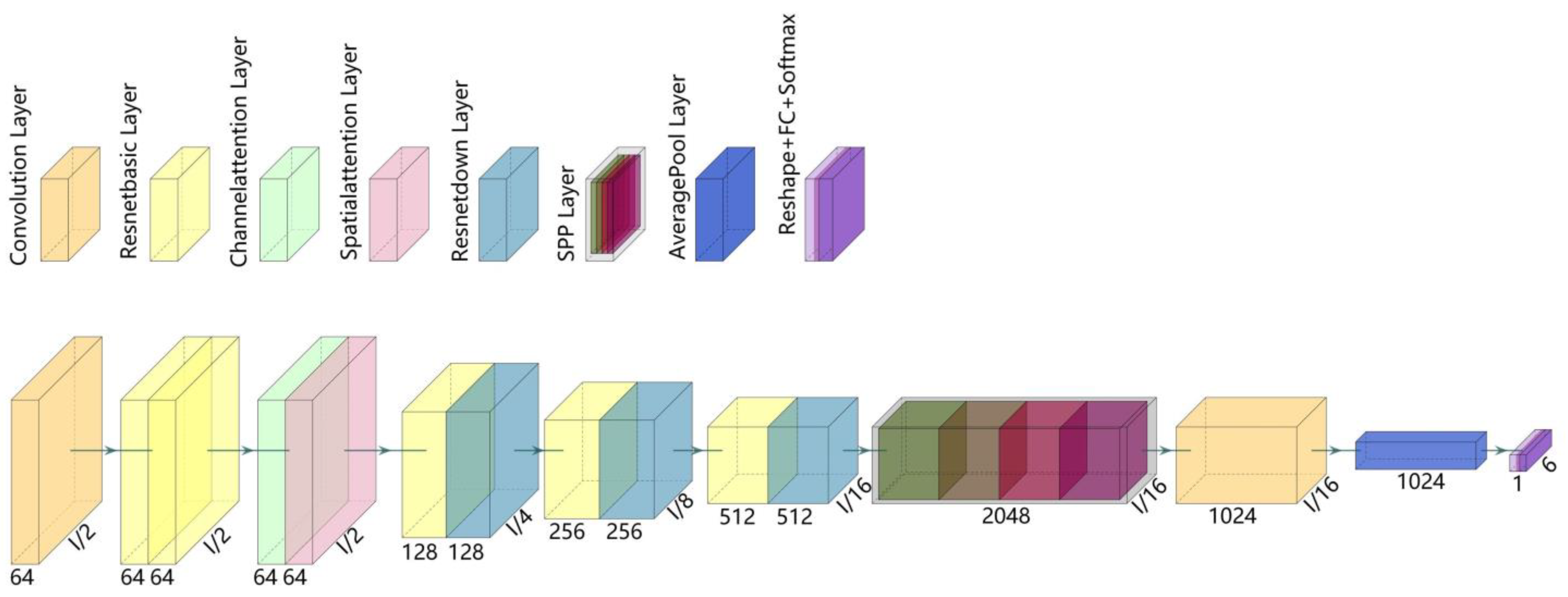
This paper proposes a model named double-attention pyramid convolutional network, which sequentially infers the mapping of attention from two independent dimensions of channel and space and realizes adaptive refinement of features. The proposed network can obtain more meaningful information. In the deeper layers of the network, it can mitigate the issue of gradient explosion stemming from heightened depth to some degree. Simultaneously, it can capture deep features across multiple scales. By combining the traits, the network model can effectively accomplish more precise and intricate classification assignments. The network architecture is shown in Figure 2.
Figure 2. Framework of attention pyramid convolution network.
Machines 11 00927 g002
The architecture consists of eight sequential layers and offers a straightforward yet efficient framework. Two consecutive ResnetbasicBlock layers create a shallow residual module, designed for shallow feature extraction. The dual-attention module, which integrates the channel attention layer with the spatial attention layer, facilitates the extraction of crucial features across both channel and spatial dimensions. Meanwhile, the deep residual module, combining the ResnetbasicBlock layer and the ResnetdownBlock layer, is tailored to mine features from deeper layers. The SPP layer is responsible for delving into vital multi-scale information from the deeper strata. A module combining the average pooling layer with a convolution operation is employed to downscale the feature dimensions transmitted by the SPP. Ultimately, after this dimensionality reduction, the reshaped features are fed into a fully connected layer paired with a SoftMax function to finalize the classification output. A detailed description of each module is provided as follows:

2.2.1. Attention Module

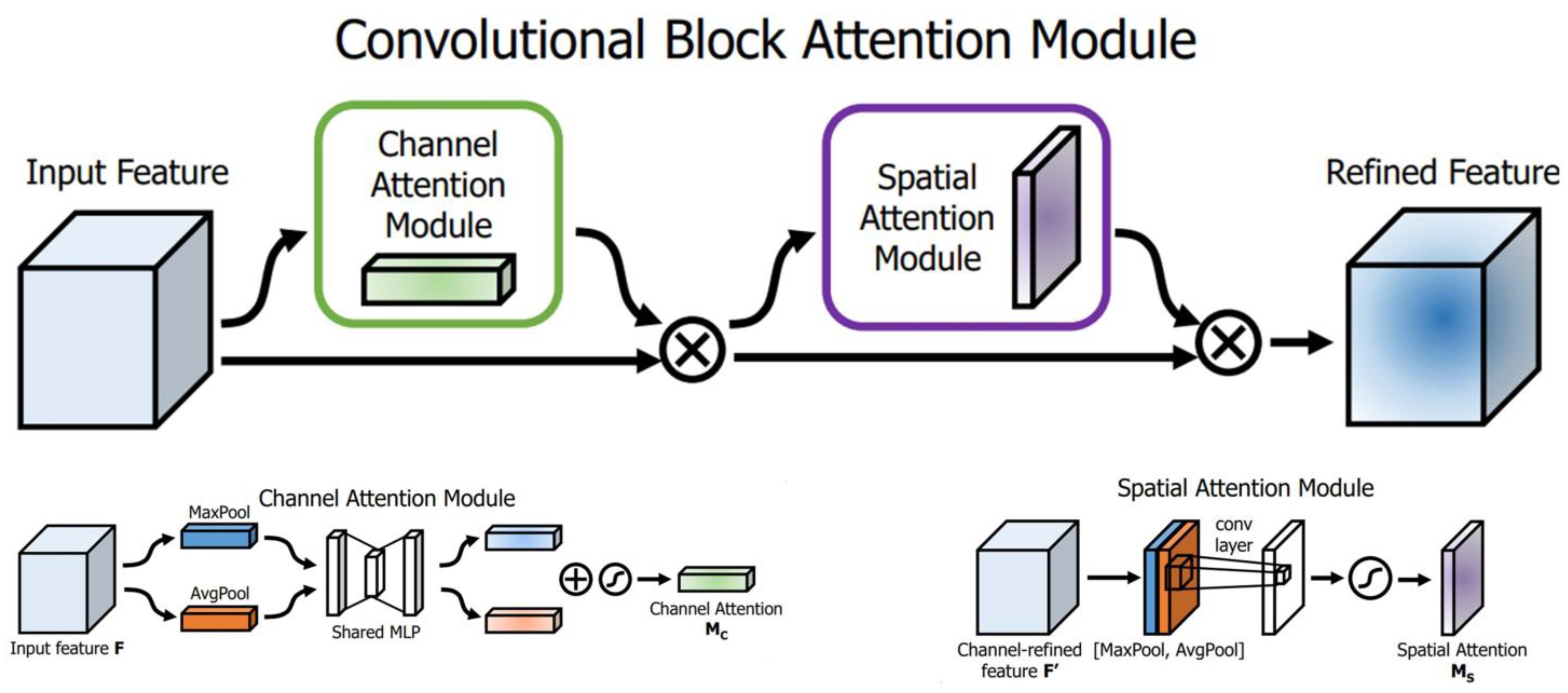
As shown in Figure 3, the attention module is mainly composed of a channel attention sub-module and a spatial attention sub-module. The principle of the channel attention mechanism is to compress the spatial information of the aggregated feature map in the spatial dimension and focus on the meaningful content of the output results in the graph. The channel attention mechanism employs both average pooling and maximum pooling techniques to aggregate spatial information from the feature map. This aggregated information is subsequently transmitted to a shared multi-layer perceptron network. The channel attention map is generated through element-wise summation and merging processes. The spatial attention mechanism is complementary to the channel attention mechanism, paying more attention to the position in the graph that is meaningful to the output. Channel attention and spatial attention are calculated as follows [26]:
M c ( F ) = σ ( W 1 ( W 0 ( F avg c ) ) + W 1 ( W 0 ( F max c ) )
M s ( F ) = σ ( f 7 × 7 [ F avg s ; F max s ] )
where σ denotes sigmoid activation function, and W 0 , W 1 are the weights of the MLP network. F avg c , F max c are the average pooling and maximum pooling features for channel attention. F avg s , F max s are the average pooling and maximum pooling features for spatial attention, respectively. f 7 × 7 denotes convolution operation and kernel size is 7 × 7 .

2.2.2. Resnet Module

With the progressive increase in the number of network layers, resulting in a deeper network architecture, the issues of gradient vanishing and gradient exploding become increasingly pronounced. To address the challenge of network degradation, residual blocks [27] are employed. As shown in Figure 4, the mapping of the residual block is F ( x ) + x = H ( x ) . H ( x ) is the desired potential mapping, and F ( x ) is the function assigned to a specific block. Assuming that optimizing the residual mapping is easier than optimizing the original and unreferenced mapping, it is much easier in extreme cases, if an identity map is optimal, to push the residuals to zero than to fit an identity map with a number of nonlinear layers. This paper employs two types of residual blocks: ResnetbasicBlock and ResnetdownBlock. The associated calculation formulas are provided below:
Y b = σ ( BN ( f 3 × 3 ( σ ( BN ( f 3 × 3 ( X b ) ) ) ) + X b )
Y d = σ ( BN ( f 3 × 3 ( σ ( BN ( f 3 × 3 ( X d ) ) ) ) + BN ( f 3 × 3 ( X d ) ) )
where X b , X d denote input features of ResnetbasicBlock and ResnetdownBlock, and Y b , Y d are output features of ResnetbasicBlock and ResnetdownBlock. f 3 × 3 , f 1 × 1 denote the convolution operation with a convolution kernel size of 3 × 3 and 1 × 1 . σ is the ReLU activate function. BN denotes layer of batch normalization.

2.2.3. Spatial Pyramid Pooling Module

In order to break the limitation of CNN on feature maps of different sizes, the spatial pyramid pooling module (SPP) [28] is introduced. Scale plays an important role in the CNN network, and the SPP can extract spatial feature information at different scales to improve the robustness of the model’s spatial layout and object variability. The SPP performed in this article is composed of three maximum pooling layers connected in parallel, and the corresponding calculation formula is as follows:
Y s = Concat ( MaxPoo l 5 × 5 ( X s ) , MaxPoo l 7 × 7 ( X s ) , MaxPoo l 13 × 13 ( X s ) )
where MaxPoo l 5 × 5 , MaxPoo l 7 × 7 , MaxPoo l 13 × 13 denote maximum pooling convolution operation with a convolution kernel size of 5 × 5 , 7 × 7 and 13 × 13 , respectively. X s , Y s are input and output features of the SPP layer. Concat denotes tensor concatenation operation.

2.3. Process of Tool Wear Identification

This paper introduces a novel method for tool wear state identification, encompassing data acquisition, preprocessing, data set partitioning, and model training and validation. The original signal is first truncated, followed by feature engineering on these truncated data. This engineering process incorporates three primary techniques: correlation analysis, principal component analysis, and feature fusion. The network model utilizes a fusion feature infographic as input. The fusion feature infographic, established after the introduction of the number of cuts with reference to the radar chart, can visualize multiple principal components of the tool wear signal feature and has time-varying characteristics. The deep CNN model has powerful feature extraction capabilities and can mine deeper features from the fusion features. In addition, interpretability analysis of CNN models with infographics as input can visualize important features that will help model classification. This tool wear classification method is illustrated in Figure 5.
The initial steps aim to establish a robust data foundation for subsequent model training and validation. As illustrated in Figure 5, following data preprocessing, a dataset is formulated specifically for the fusion feature infographic and is partitioned into training and testing datasets. The training dataset facilitates the network model’s training, while the testing dataset assesses the model’s performance. Notably, the network model can promptly and precisely determine tool wear state based on the fusion feature infographic input.

3. Experiment Setup

3.1. Machining Device and Data Acquisition

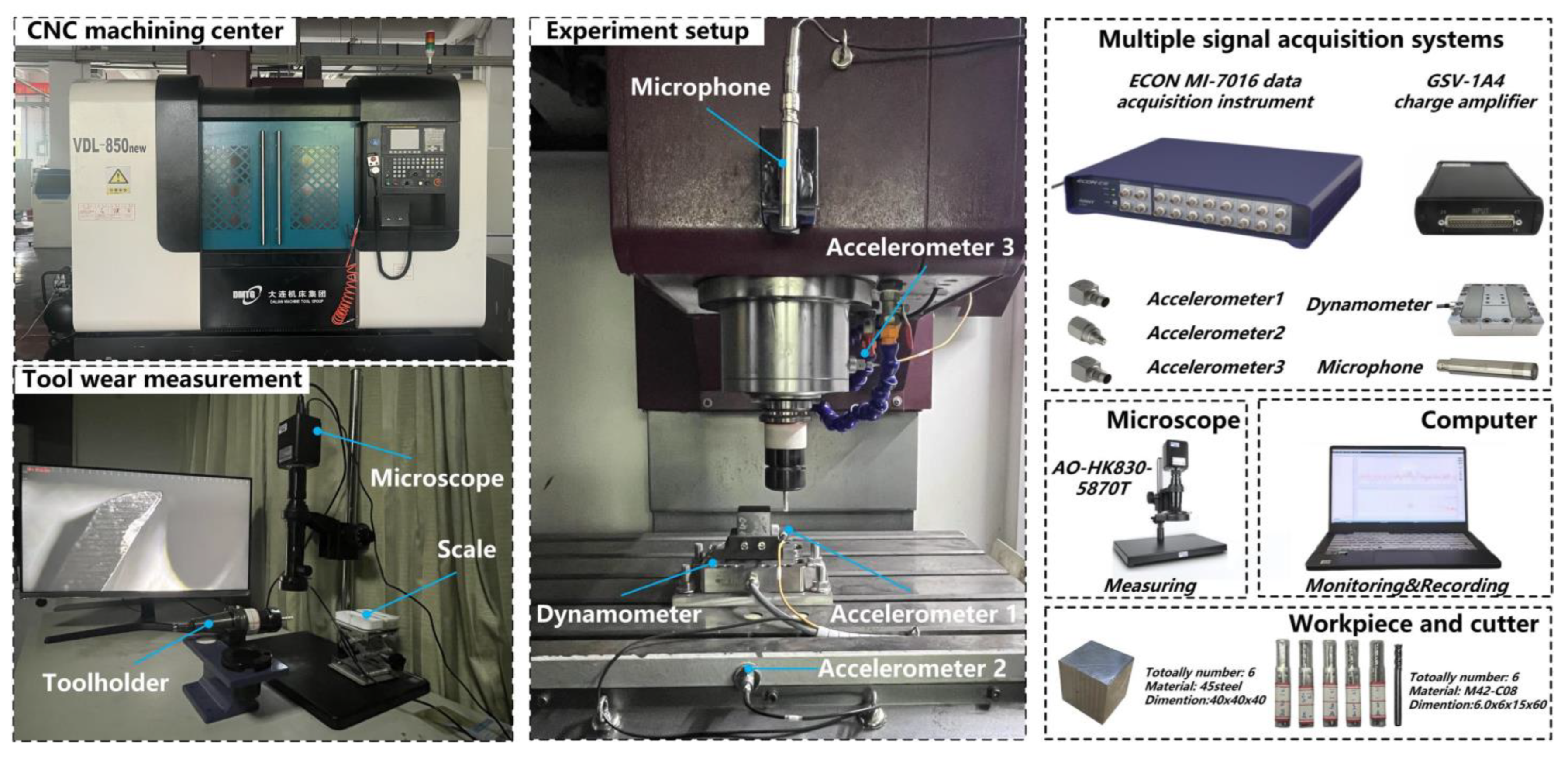
The experimental setup employed in this study is depicted in Figure 6. The tool wear experiment was conducted using the VDL-850 New CNC machining center from Dalia- n Machine Tool Factory. Tool wear was measured using the AOSVI HK830-5870T micro-scope. The ECON MI-7016 data acquisition instrument was utilized to record force vibration, and sound signals during the cutting process. Two triaxial acceleration sensors were magnetically attached to the workpiece and the machining center’s spindle. Then, a uniaxial acceleration sensor was magnetically affixed to the worktable, and a microphone was anchored to the table via a magnetic base and bracket. The force sensor was positioned between a custom-designed fixture and the worktable using an adapter plate. The tri-axial acceleration sensors on the workpiece exhibited sensitivities of 101.49 mv/g, 99.44 mv/g, and 99.89 mv/g, while those on the spindle had sensitivities of 97.82 mv/g, 101.27 mv/g, and 100.58 mv/g. The uniaxial acceleration sensor on the worktable demonstrated a sensitivity of 99.71 mv/g and the microphone exhibited a sensitivity of 45.18 mv/Pa. The force sensor had a range of up to 2000 N. The cutting tool employed was a SKT cobalt-enriched high-speed steel integral end mill, with the workpiece being composed of 45 steel.
As depicted in Figure 6, the workpiece dimensions were 40 mm × 40 mm × 40 mm. The tool possessed four blades, each with a diameter of 6.0 mm and a length of 15.0 mm, culminating in a total tool length of 60.0 mm. Six tools and workpieces were employed in the experiment. Detailed parameters for the study can be found in Table 1. The experiment focused on face milling with consistent cutting parameters, utilizing dry cutting. The A wx A wy and A wz signals were derived from accelerometer 1, and the A sx , A sy and A sz signals were derived from accelerometer 3. The A o and V o signals were derived from accelerometer 2 and the microphone, respectively.
To balance acquisition time and efficiency, a sampling frequency of 20,400 Hz was set for each channel.
The force sensor in the experiment served to detect tool overloads and assisted in tool positioning. However, its data were not consistently recorded throughout the experiment. Both the acceleration sensor and the microphone were connected to the data acquisition instrument via BNC connectors. Conversely, the force sensor was linked through a charge amplifier. The data acquisition instrument then relayed the collected signals from the cutting process to a laptop for monitoring and recording.

3.2. Measurement of Tool Flank Wear VB

According to the amount of material removed, up to 4 mm 3 per cut, the signal generated by each cutting was recorded and the wear condition of the tool was subsequently measured. Tool wear during milling predominantly occurs on the flanks of the end and side cutting edges. Multiple metrics gauge tool wear. These include one-dimensional metrics such as average and maximum wear bandwidth, tool nose radius; two-dimensional metrics such as the wear zone area and the crescent wear area; and three-dimensional metrics such as the tool tip wear volume. Extensive experimentation reveals that side wear on the milling cutter is more easily observed and quantified than end wear. Consequently, the maximum bandwidth of the side blade’s flank wear zone is chosen as the wear measurement indicator, consistent with [29]. Given the variability in wear bandwidth across the milling cutter’s edges, an average wear value is derived from measurements on each edge to provide a balanced assessment. The associated computation is delineated below:
VB = i = 1 N V B Ci N
where V B C i denotes the wear value of the i-th blade and N denotes the total number of blades. VB is used to characterize the wear value of the entire tool.
To measure the wear value of each blade and to consider the field of view, measurement accuracy, and ambient illumination of the microscope, the magnification was set to a 1× scale. The impact of ambient light on the measurement was minimized by adjusting the intensity of the ring light source during the process. Out of the six tools used in the cutting experiment, only three displayed the anticipated tool wear. These tools were designated as Tool 1, Tool2, and Tool 3. Tool1 serves as a representative example to delineate the categorization of tool wear status and the VB measurement technique.
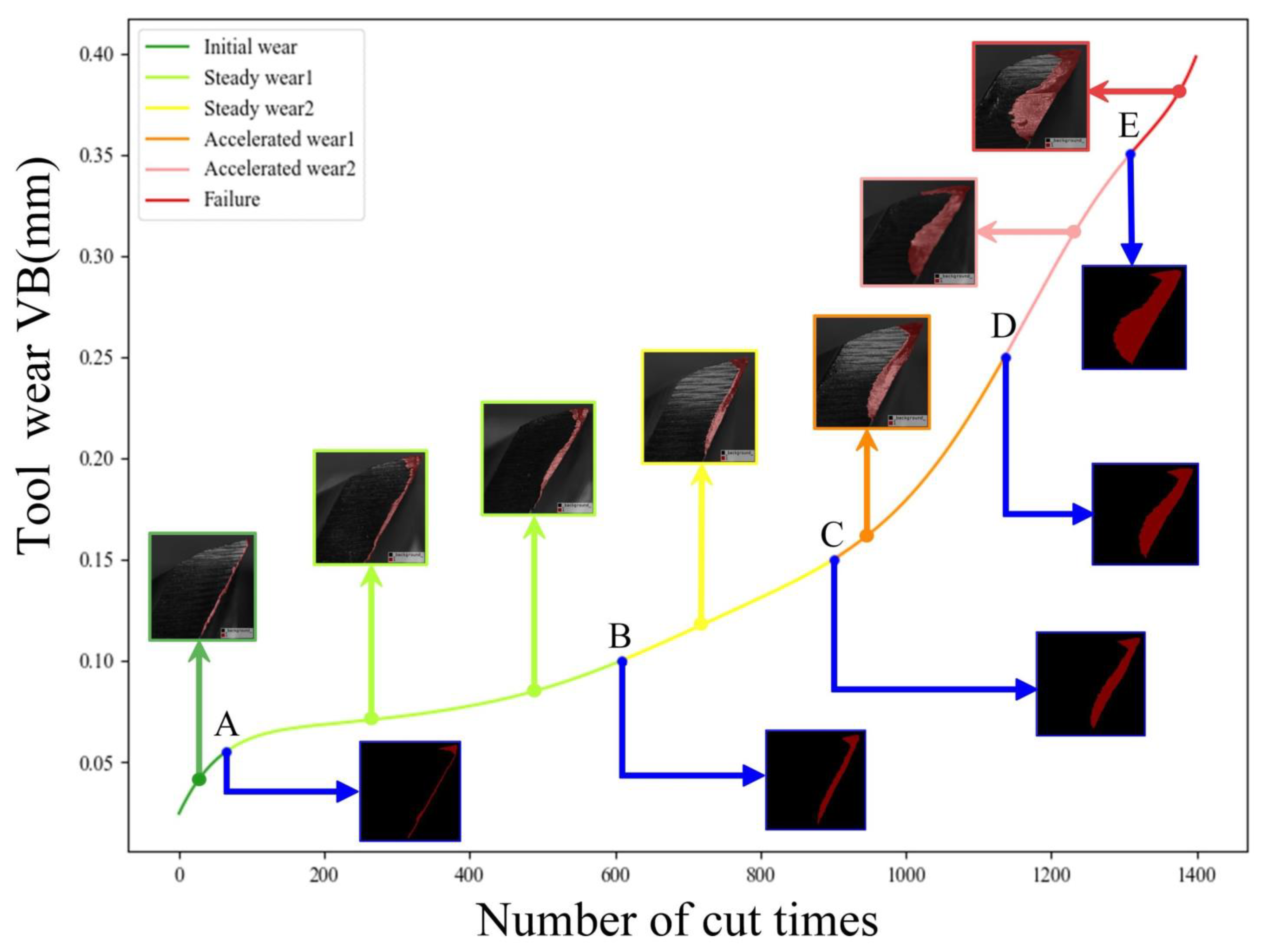
Figure 7 displays the wear progression of Tool1′s VB relative to the number of cuts, illustrating an increase in tool wear VB with more cuts. The tool’s wear state is determined with respect to its wear rate. Transition points A, B, C, D, and E in Figure 7 represent transition points of various tool wear states. The images above the curve portray the tool’s wear in distinct states, with the red section indicating the wear area. Conversely, the images beneath the curve show tool wear morphology at the transition points. For clarity, only the segmented wear regions have been retained at these transition points. It should be noted that they are all derived from the same measuring instrument, but with different image processing. As delineated in Table 2, the tool’s wear state is segmented into six states: initial wear, steady wear 1, steady wear 2, accelerated wear 1, accelerated wear 2, and failure. The table’s final column corresponds to the VB range for each wear state.
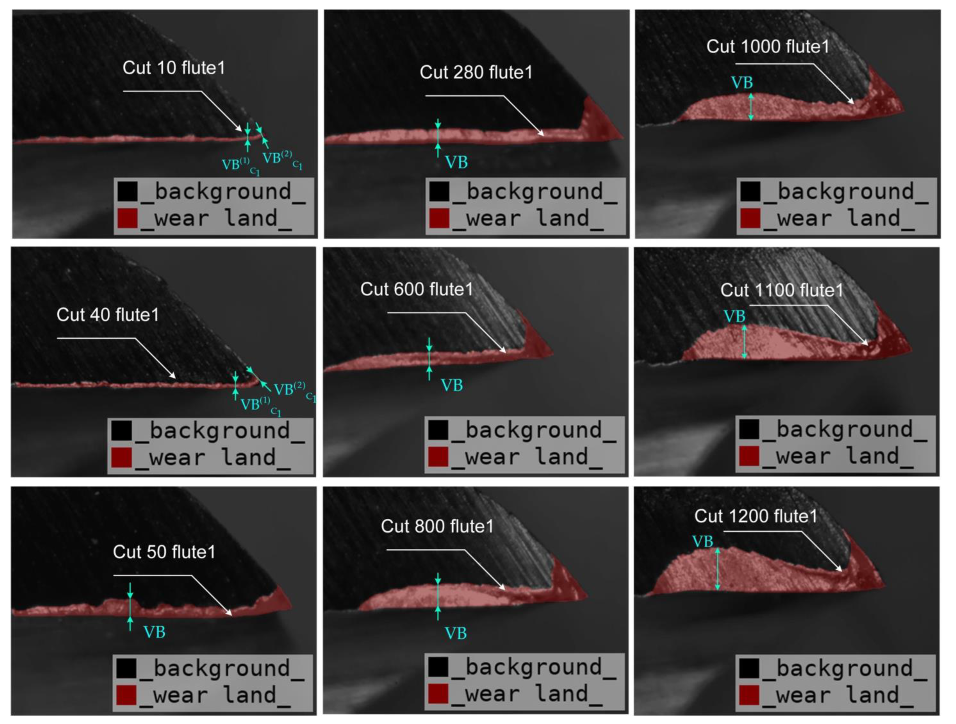
Figure 8 illustrates the measurement method for tool wear, denoted as VB, under various cutting durations. Extensive experimentation revealed that the wear shape transformation for the cutting edge remains consistent across different instances and the rate of this transformation varies. As such, the figure presents the measurement method for VB during different cutting times for a single tooth, with the wear area’s shape evolution also depicted therein. In the initial wear phase, wear is predominantly localized at the blade tip. Therefore, the measured part is selected at the tip of the tool. During this phase, the formula for VB is given as:
VB = max { V B ( 1 ) C 1 , V B ( 2 ) C 1 }
As cutting progresses, the wear area swiftly develops and broadens, eventually surpassing the blade’s front and tip. During the stable wear phase, the rate of wear decelerates, but wear continues. Notably, as the tool approaches the accelerated wear phase, pronounced crescent-shaped pits emerge near the half-depth of the cut. Upon reaching the accelerated wear phase, the wear region surrounding the pit expands dramatically until tool breakdown occurs. Figure 8 also details the VB measurement method for the stable and accelerated wear stages, and for tool failure.

3.3. Experimental Data Preprocessing

As highlighted in Section 2.1, the gathered acoustic vibration signal undergoes processes such as truncation and feature engineering to be transformed into a feature fusion infographic. This facilitates the conversion of one-dimensional data into their two-dimensional counterparts. A 3-second segment is extracted from the original acoustic vibration signal, enhancing data quality by excluding signals related to the commencement of cutting, its termination, and the uncut phase. The infographic, based on the refined signal and the count of cutting instances, serves as the dataset. The distribution of numbers for different categories within this dataset is detailed in Table 3. Following data preprocessing, the dataset undergoes a random partitioning into training and test subsets at an 8:2 ratio. The training dataset exclusively serves the purpose of network training for weight updating, with a random selection of 200 samples from the 800 training samples designated as the validation set. Consequently, the input network’s tensor shape stands at 600 × 3 × 224 × 224. The input data undergoes batch processing with 256 images to augment the network’s training velocity. Finally, the testing data set aids in assessing the performance of the model.

4. Results and Discussion

4.1. Results of Model Training

It should be noted that the data used in the training and testing were all derived from the same CNC machining center. The training experiments were conducted within the Anaconda virtual environment, utilizing Python 3.8 and frameworks such as PyTorch 1.12 and CUDA 11.6.
Table 4 lists the hyperparameters used for training, which include an epoch count of 100, a batch size of 256, and a specified learning rate. All models undergoing training employed identical hyperparameters. Throughout the training phase, various image enhancements, including central cropping and pixel normalization, were applied to the fusion feature infographic. These enhanced data were subsequently fed into four deep convolutional neural networks. The RMSprop optimization algorithm [30] consistently updated the network weights to minimize the loss function. Figure 9 presents the loss and accuracy curves for the proposed model during training. Remarkably, the model reached peak performance within a limited number of epochs. As demonstrated in Figure 9a, the accuracy stabilizes at a notable 97.98%, while the loss remains between 0 and 1 as shown in Figure 9b. To accentuate the proposed model’s superiority, comparison networks, namely LeNet [31], Resnet18, and VGG16 [32], were also implemented.
This study utilizes metrics derived from the confusion matrix [33] to evaluate the model’s efficacy in wear level classification tasks. These metrics encompass accuracy, precision, recall, and the F1 score. Accuracy measures the fraction of correct predictions across all samples. Precision quantifies the ratio of accurate predictions to all predicted outcomes, while recall captures the proportion of accurate predictions relative to actual results. It is worth noting that precision and recall typically demonstrate a trade-off; however, the F1 score adeptly harmonizes these metrics. The computation formulae for these indicators are provided below:
Accuracy = TP + TN TP + TN + FP + FN
Precision = TP TP + FP
Recall = TP TP + FN
F 1 - score = 2 × Precision × Recall Precision + Recall
where TP denotes the number of positive cases correctly identified, FP represents the number of positive cases incorrectly identified, TN represents the number of negative cases correctly identified, and FN represents the number of negative cases incorrectly identified.
Figure 10 depicts the confusion matrices of various models evaluated on the test set. Such matrices facilitate error analysis and elucidation of category-specific ambiguities. In these matrices, each cell indicates the model’s predictive outcome juxtaposed against the actual wear state. Every row signifies predictions for a specific wear category, and each column denotes the true category. Notably, diagonal cells signify the accurate classifications for each wear state. According to Figure 10, the classification accuracy for the six wear states in the proposed model surpasses that of its counterparts, boasting an impressive average accuracy of 97.83%.
The results for the four networks on the test set are detailed in Table 5. While the proposed model exhibits a longer processing time compared with the Resnet18 baseline, it surpasses it in terms of classification accuracy and precision. The inclusion of the attention module and pyramid convolutional pooling layers brings about extra parameters, potentially increasing computational overhead. However, the attention module accentuates the intensity data of both spatial and channel features, whereas the pyramid convolutional pooling layer assimilates crucial multi-scale data, enhancing the model’s classification accuracy. As depicted in Table 5, the proposed model outperforms the comparator models in all aspects except processing time. The model registers an accuracy of 97.98%, a precision of 97.87%, a recall rate of 97.80%, and an F1 score of 97.83%. Relative to the baseline, there is an augmentation of 12.6% in accuracy, 9.97% in precision, and 13.4% in the F1 score. Thus, the introduced model strikes a harmonious balance between speed and quality, optimizing both accuracy and time efficiency.

4.2. Neural Network Interpretability Analysis

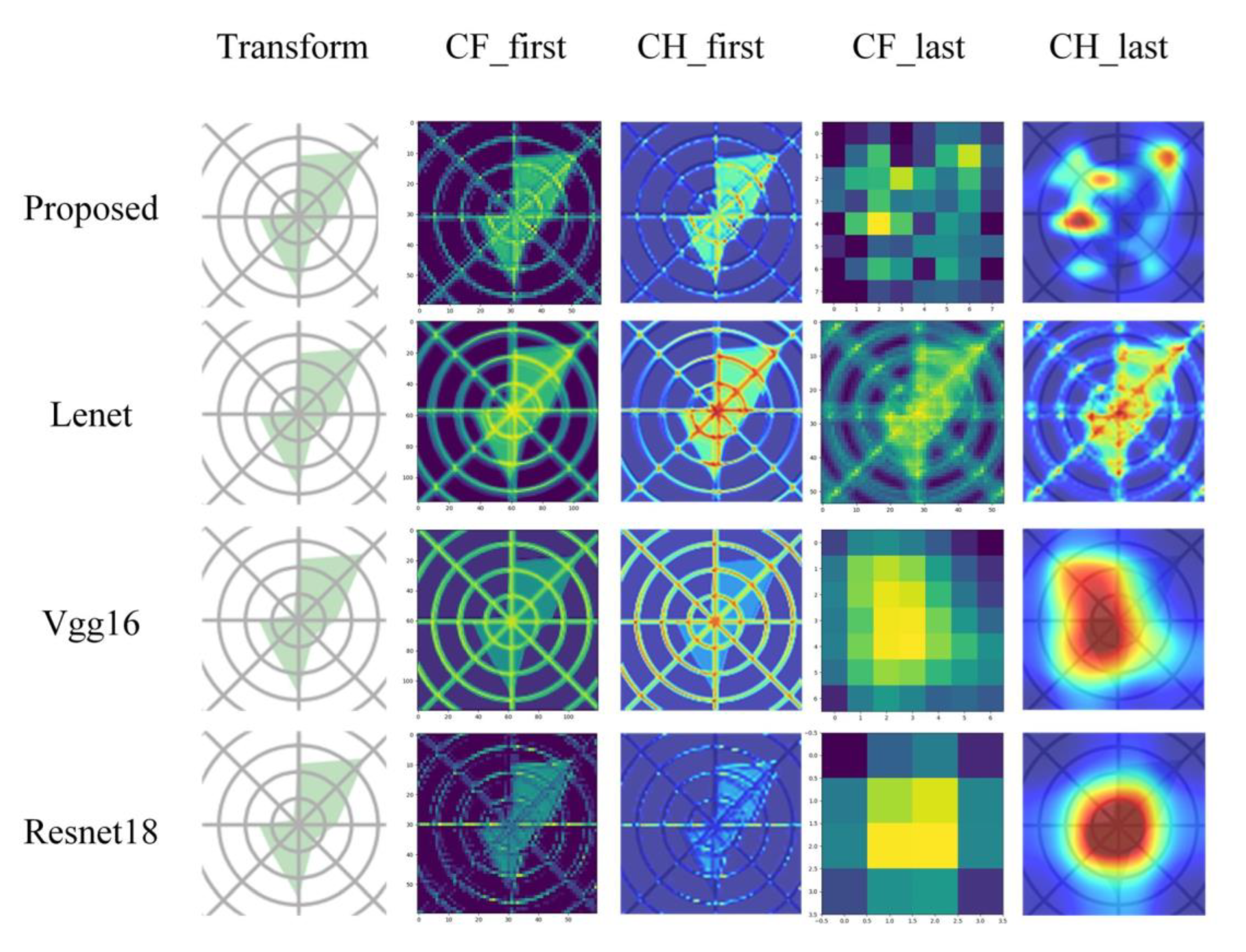
The proposed model is adept at discerning crucial intricate details within images. The visualization results of the activation heat map [34] for the feature fusion map are shown below. The rendition in Figure 11 shows the image post-preprocessing for the feature fusion map prior to network input. ‘CF_first’ and ‘CF_last’ denote the class activation heatmaps for the initial and concluding convolutional layers of the network, respectively. Similarly, ‘CH_first’ and ‘CH_last’ represent the class activation heatmaps of the first and last convolutional layers superimposed on the original image. These class activation maps elucidate the weight distribution of the adaptive multi-scale prediction fusion. Within the class activation map, regions highlighted in yellow signify important features retained post-convolution; the deeper the hue of yellow, the more significant the feature. When superimposed on the original image, regions marked in red within the class activation map indicate pivotal influences on the category output, with deeper shades of red denoting increased importance.
As depicted in Figure 11, Lenet, Vgg16, and the superficial layers of the proposed network tend to prioritize the grid lines of the information graph. This observation underscores that either shallow networks or the initial layers of more profound networks frequently emphasize the significance of grid lines encompassed by the information graph’s outline for the accurate categorization of wear states. As the depth of the network increases, it becomes evident that the profound layers of networks like Vgg16 and Resnet18 focus more on the inner contours encircled by the fusion features within the information graph. Within the class activation heat map of the network presented in this study, a pronounced red region near the fusion feature and intrinsic feature values indicates their pivotal role in accurately discerning tool wear state identification. Furthermore, Figure 11 elucidates that the proposed network adeptly discerns the interrelation between pixels and channels in images, attesting to the efficacy of the proposed network model. This ensures an optimal allocation of features related to accurate wear categorization without compromising vital graph information. To sum up, the class activation heat maps from various networks reveal that the proposed model’s shallow layer perceives the inner contours delineated by the fusion features or the inner grid lines as pivotal. Conversely, its deeper layers prioritize areas proximate to the fused feature values on the information graph, reinforcing the model’s effectiveness.

5. Conclusions and Future Work

Comprehensive experiments and model comparisons validate the efficacy of the method of identification of tool wear. There are some conclusions as follows:
1. The proposed vibroacoustic signal fusion feature infographic effectively amalgamates information directly related to tool wear. It not only minimizes noise interference from signal features but also captures the dynamic attributes of the cutting process.
2. The double-attention mechanism applied in our proposed model focusing on channels and spatial aspects adaptively perceives network weight for infographics associated with wear categories. Notably, when benchmarked against Resnet18, the double-attention model built on infographics elevates the F1 score by 13.4%, exhibiting superior accuracy, precision, and recall.
In future work, because of the inconsistent dynamic nature of machine tools, we will collect data from different machine tools under different cutting conditions to augment the dataset to enhance the robustness of the model.
Author Contributions

Conceptualization, X.L. and J.N.; methodology, X.L.; software, X.L.; validation, X.L., Z.M. and Y.C.; formal analysis, X.L.; investigation, X.L. and Z.M.; resources, J.N.; data curation, X.L. and J.N.; writing—original draft preparation, X.L.; writing—review and editing, X.L., J.N. and Z.M.; visualization, X.L. and J.N.; supervision, J.N.; project administration, X.L. and J.N.; funding acquisition, X.L. and J.N. All authors have read and agreed to the published version of the manuscript.

Funding

This research was funded by National Natural Science of Foundation of China (Grant No. U21A20134), Natural Science of Foundation of Zhejiang Province (Grant No. LR20E05000).

Institutional Review Board Statement

Not applicable.

Informed Consent Statement

Not applicable.

Data Availability Statement

The data are not publicly available due to privacy and commercial restrictions.

Conflicts of Interest

The authors declare no conflict of interest.

Appendix A

Table A1. Features extracted in time domain.
FeatureExpressionFeatureExpression
Mean F 1 = 1 N i = 1 N x i Pulse factor F 9 = max { i [ 1 , N ] } ( 1 F 1 | x i | )
Standard deviation F 2 = 1 N i = 1 N ( x i - F 1 ) 2 Margin factor F 10 = 1 F 8 max ( | x i | ) { i [ 1 , N ] }
Skewness F 3 = 1 N i = 1 N [ ( x i - F 1 F 2 ) 3 ] Energy F 11 = i = 1 N | x i 2 |
Kurtosis F 4 = 1 N i = 1 N ( x i - F 1 F 2 ) 4 Average absolute value F 12 = 1 N i = 1 N | x i |
Peak-to-peak F 5 = max ( x i ) { i [ 1 , N ] } - min ( x i ) { i [ 1 , N ] } Variance F 13 = 1 N - 1 i = 1 N ( x i - F 1 ) 2
Root mean square F 6 = 1 N i = 1 N x i 2 Root amplitude F 14 = ( 1 N i = 1 N | x i | ) 2
Crest factor F 7 = F 6 F 5 Peak value F 15 = max ( | x i | ) { i [ 1 , N ] }
Form factor F 8 = 1 F 6 max ( | x i | ) { i [ 1 , N ] } Maximum and Minimum F 16 = max ( x i ) { i [ 1 , N ] } F 17 = min ( x i ) { i [ 1 , N ] }
Table A2. Features extracted in frequency domain. p and PSD in the table represent the amplitude spectrum and the power spectrum, respectively. f b represents the rotation frequency of the spindle.
FeatureExpressionFeatureExpression
Average amplitude S 1 = 1 N k = 1 N p ( f k ) Medium frequency S 7 = 1 2 0 + PSD ( f ) df
Gravity frequency S 2 = k = 1 N f k p ( f k ) k = 1 N p ( f k ) Total power S 8 = k = 1 N PSD ( f k )
Mean square frequency S 3 = k = 1 N f k 2 p ( f k ) k = 1 k p ( f k ) Average power S 9 = S 8 N
Frequency variance S 4 = k = 1 N ( f k - S 2 ) 2 p ( f k ) k = 1 N p ( f k ) Maximum power frequency S 10 = argmax ( PSD ( f ) )
Frequency amplitude variance S 5 = k = 1 N ( f k ) 2 p ( f k ) k = 1 N p ( f k ) Low to high power ratio S 11 = 0 b PSD ( f ) df b + PSD ( f ) df , b = 3 f b
Mean frequency S 6 = 0 + f PSD ( f ) df 0 + PSD ( f ) df
Table A3. Features extracted in time-frequency domain. W T j and W T R j in the table represent the wavelet packet coefficient and the reconstructed wavelet packet coefficient, respectively.
FeatureExpression
Wavelet energy ratio E j = i = 1 N W T R j 2 ( i ) j = 1 M i = 1 N W T R j 2 ( i ) , W 1 = E 1 , W 2 = E 2 , , W 8 = E 8
Wavelet energy spectral entropy W 9 = - j = 1 M E j log E j
Wavelet-scale entropy D j = - i = 1 N / 8 W T j 2 ( i ) log W T j 2 ( i ) , W 10 = D 1 , W 11 = D 2 , , W 17 = D 8
Wavelet singular spectral entropy Q j = SVD ( W T R j ) j = 1 M SVD ( W T R j ) , W 18 = - j = 1 M Q j log Q j

References

  1. Erden, M.A.; Yaşar, N.; Korkmaz, M.E.; Ayvacı, B.; Nimel Sworna Ross, K.; Mia, M. Investigation of microstructure, mechanical and machinability properties of Mo-added steel produced by powder metallurgy method. Int. J. Adv. Manuf. Technol. 2021, 114, 2811–2827. [Google Scholar] [CrossRef]
  2. Zhang, T.; Zhang, C.; Wang, Y.; Zou, X.; Hu, T. A vision-based fusion method for defect detection of milling cutter spiral cutting edge. Measurement 2021, 177, 109248. [Google Scholar] [CrossRef]
  3. Wiklund, H. Bayesian and regression approaches to on-line prediction of residual tool life. Qual. Reliab. Eng. Int. 1998, 14, 303–309. [Google Scholar] [CrossRef]
  4. Kious, M.; Ouahabi, A.; Boudraa, M.; Serra, R.; Cheknane, A. Detection process approach of tool wear in high speed milling. Measurement 2010, 43, 1439–1446. [Google Scholar] [CrossRef]
  5. Jaini, S.N.B.; Lee, D.-W.; Lee, S.-J.; Kim, M.-R.; Son, G.-H. Indirect tool monitoring in drilling based on gap sensor signal and multilayer perceptron feed forward neural network. J. Intell. Manuf. 2021, 32, 1605–1619. [Google Scholar] [CrossRef]
  6. Kerr, D.; Pengilley, J.; Garwood, R. Assessment and visualisation of machine tool wear using computer vision. Int. J. Adv. Manuf. Technol. 2006, 28, 781–791. [Google Scholar] [CrossRef]
  7. Kassim, A.A.; Mannan, M.A.; Mian, Z. Texture analysis methods for tool condition monitoring. Image Vis. Comput. 2007, 25, 1080–1090. [Google Scholar] [CrossRef]
  8. Zhou, J.; Yue, C.; Liu, X.; Xia, W.; Wei, X.; Qu, J.; Liang, S.Y.; Wang, L. Classification of Tool Wear State based on Dual Attention Mechanism Network. Robot. Comput. Integr. Manuf. 2023, 83, 102575. [Google Scholar] [CrossRef]
  9. Silva, R.G.; Baker, K.J.; Wilcox, S.J.; Reuben, R.L. The Adaptability of a Tool Wear Monitoring System under Changing Cutting Conditions. Mech. Syst. Signal Process. 2000, 14, 287–298. [Google Scholar] [CrossRef]
  10. Wang, C.; Bao, Z.; Zhang, P.; Ming, W.; Chen, M. Tool wear evaluation under minimum quantity lubrication by clustering energy of acoustic emission burst signals. Measurement 2019, 138, 256–265. [Google Scholar] [CrossRef]
  11. Loenzo, R.A.G.; Lumbreras, P.D.A.; Troncoso, R.d.J.R.; Ruiz, G.H. An object-oriented architecture for sensorless cutting force feedback for CNC milling process monitoring and control. Adv. Eng. Softw. 2010, 41, 754–761. [Google Scholar] [CrossRef]
  12. Li, Z.; Liu, X.; Incecik, A.; Gupta, M.K.; Królczyk, G.M.; Gardoni, P. A novel ensemble deep learning model for cutting tool wear monitoring using audio sensors. J. Manuf. Process. 2022, 79, 233–249. [Google Scholar] [CrossRef]
  13. Zhou, Y.; Sun, B.; Sun, W. A tool condition monitoring method based on two-layer angle kernel extreme learning machine and binary differential evolution for milling. Measurement 2020, 166, 108186. [Google Scholar] [CrossRef]
  14. Prakash, K.; Samraj, A. Tool flank wears estimation by simplified SVD on emitted sound signals. In Proceedings of the 2017 Conference on Emerging Devices and Smart Systems (ICEDSS), Nāmakkal, India, 3–4 March 2017; pp. 1–5. [Google Scholar]
  15. Shi, C.; Luo, B.; He, S.; Li, K.; Liu, H.; Li, B. Tool Wear Prediction via Multidimensional Stacked Sparse Autoencoders With Feature Fusion. IEEE Trans. Ind. Inform. 2020, 16, 5150–5159. [Google Scholar] [CrossRef]
  16. Twardowski, P.; Czyżycki, J.; Felusiak-Czyryca, A.; Tabaszewski, M.; Wiciak-Pikuła, M. Monitoring and forecasting of tool wear based on measurements of vibration accelerations during cast iron milling. J. Manuf. Process. 2023, 95, 342–350. [Google Scholar] [CrossRef]
  17. Bahador, A.; Du, C.; Ng, H.P.; Dzulqarnain, N.A.; Ho, C.L. Cost-effective classification of tool wear with transfer learning based on tool vibration for hard turning processes. Measurement 2022, 201, 111701. [Google Scholar] [CrossRef]
  18. Wang, P.; Gao, R.X. Transfer learning for enhanced machine fault diagnosis in manufacturing. CIRP Ann. 2020, 69, 413–416. [Google Scholar] [CrossRef]
  19. Li, X.; Liu, X.; Yue, C.; Liang, S.Y.; Wang, L. Systematic review on tool breakage monitoring techniques in machining operations. Int. J. Mach. Tools Manuf. 2022, 176, 103882. [Google Scholar] [CrossRef]
  20. Rafezi, H.; Akbari, J.; Behzad, M. Tool Condition Monitoring based on sound and vibration analysis and wavelet packet decomposition. In Proceedings of the 2012 8th International Symposium on Mechatronics and its Applications, Sharjah, United Arab Emirates, 10–12 April 2012; pp. 1–4. [Google Scholar]
  21. Gomes, M.C.; Brito, L.C.; Bacci da Silva, M.; Viana Duarte, M.A. Tool wear monitoring in micromilling using Support Vector Machine with vibration and sound sensors. Precis. Eng. 2021, 67, 137–151. [Google Scholar] [CrossRef]
  22. Niaki, F.; Feng, L.; Ulutan, D.; Mears, L. A wavelet-based data-driven modelling for tool wear assessment of difficult to machine materials. Int. J. Mechatron. Manuf. Syst. 2016, 9, 97–121. [Google Scholar] [CrossRef]
  23. Niu, B.; Sun, J.; Yang, B. Multisensory based tool wear monitoring for practical applications in milling of titanium alloy. Mater. Today Proc. 2020, 22, 1209–1217. [Google Scholar] [CrossRef]
  24. Pearson, K. On lines and planes of closest fit to systems of points in space. Philos. Mag. 1901, 2, 559–572. [Google Scholar] [CrossRef]
  25. Ma, Y.Z. A Tutorial on Principal Component Analysis. arXiv 2014, arXiv:1404.1100. [Google Scholar]
  26. Woo, S.; Park, J.; Lee, J.-Y.; Kweon, I. CBAM: Convolutional Block Attention Module. In Proceedings of the 15th European Conference, Munich, Germany, 8–14 September 2018; Proceedings, Part VII. pp. 3–19. [Google Scholar]
  27. He, K.; Zhang, X.; Ren, S.; Sun, J. Deep Residual Learning for Image Recognition. In Proceedings of the IEEE Conference on Computer Vision and Pattern Recognition (CVPR), Las Vegas, NV, USA, 27–30 June 2016; pp. 770–778. [Google Scholar]
  28. He, K.; Zhang, X.; Ren, S.; Sun, J. Spatial pyramid pooling in deep convolutional networks for visual recognition. IEEE Trans. Pattern Anal. Mach. Intell. 2015, 37, 1904–1916. [Google Scholar] [CrossRef] [PubMed]
  29. Kong, D.; Chen, Y.; Li, N. Gaussian process regression for tool wear prediction. Mech. Syst. Signal Process. 2018, 104, 556–574. [Google Scholar] [CrossRef]
  30. Ruder, S.J.A. An overview of gradient descent optimization algorithms. arXiv 2016, arXiv:1609.04747. [Google Scholar]
  31. Lecun, Y.; Bottou, L.; Bengio, Y.; Haffner, P. Gradient-Based Learning Applied to Document Recognition. Proc. IEEE 1998, 86, 2278–2324. [Google Scholar] [CrossRef]
  32. Simonyan, K.; Zisserman, A. Very Deep Convolutional Networks for Large-Scale Image Recognition. In Proceedings of the International Conference on Learning Representations, San Diego, CA, USA, 7–9 May 2015. [Google Scholar]
  33. Salmon, B.P.; Kleynhans, W.; Schwegmann, C.P.; Olivier, J.C. Proper comparison among methods using a confusion matrix. In Proceedings of the 2015 IEEE International Geoscience and Remote Sensing Symposium (IGARSS), Milan, Italy, 26–31 July 2015; pp. 3057–3060. [Google Scholar]
  34. Selvaraju, R.R.; Cogswell, M.; Das, A.; Vedantam, R.; Parikh, D.; Batra, D. Grad-CAM: Visual Explanations from Deep Networks via Gradient-based Localization. arXiv 2016, arXiv:1610.02391. [Google Scholar] [CrossRef]
Figure 1. The establishment process of vibroacoustic signal fusion feature infographics: (a) correlation analysis; (b) data dimensionality reduction; (c) fusion feature infographic. C1 in Figure 1a represents tool 1 in Section 3.2, and Wy represents the channel of the work piece vibration signal in the y-axis direction in Section 3.1.
Machines 11 00927 g001
Figure 3. Internal details of attention module [26].
Machines 11 00927 g003
Figure 4. Residual Block: a building block.
Machines 11 00927 g004
Figure 5. Method flow of proposed tool wear state identification.
Machines 11 00927 g005
Figure 6. Experiment setup for milling experiment, tool wear measurement and signal data acquisition.
Machines 11 00927 g006
Figure 7. Tool wear curve relative to cutting times.
Machines 11 00927 g007
Figure 8. Flank wear images under different cutting times and the measurement of VB.
Machines 11 00927 g008
Figure 9. Training results of proposed model: (a) accuracy curve; (b) loss curve.
Machines 11 00927 g009
Figure 10. Confusion matrices of different models.
Machines 11 00927 g010
Figure 11. Class activation heat maps of different networks.
Machines 11 00927 g011
Table 1. Detailed parameters of the experimental operation.
ObjectParameter Value
Signal channels A wx , A wy , A wz , A o , A sx , A sy , A sz , V o
Sampling frequency20,400 Hz/channel
Spindle speed800 r/min
Longitudinal feed400 mm/min
Axial depth of cut0.1 mm
Radial depth of cut1 mm
Table 2. Tool wear state.
Wear StateCategoryTool Flank Wear VB (mm)
Initial wear00~0.05
Steady wear 110.05~0.10
Steady wear 220.10~0.15
Accelerated wear 130.15~0.25
Accelerated wear 240.25~0.35
Failure5>0.35
Table 3. Number of samples from each category in the dataset.
CategoryNumber of Samples
Tool 1Tool 2Tool 3
012150120
1235559360
2180292210
3264236300
4170174150
5819015
Table 4. Training parameters of models.
ParametersLenetResnet18VGG16Proposed
Epoch100100100100
Batch size256256256256
Learning rate0.000010.000010.000010.00001
OptimizationRMSpropRMSpropRMSpropRMSprop
Smoothing constant0.990.990.990.99
Table 5. Comparison of network model performance.
ModelAccuracyPrecisionRecallF1 ScoreTest-Time
LeNet92.81%93.62%92.24%92.92%0.011 s
Resnet1887.01%89.00%83.62%86.22%0.007 s
VGG1693.36%93.42%92.23%92.82%0.028 s
proposed97.98%97.87%97.80%97.83%0.024 s
Disclaimer/Publisher’s Note: The statements, opinions and data contained in all publications are solely those of the individual author(s) and contributor(s) and not of MDPI and/or the editor(s). MDPI and/or the editor(s) disclaim responsibility for any injury to people or property resulting from any ideas, methods, instructions or products referred to in the content.