Article

Comparative Analysis of Data-Driven Models for Marine Engine In-Cylinder Pressure Prediction

by
Chaitanya Patil
and
Gerasimos Theotokatos
*
Maritime Safety Research Centre, Department of Naval Architecture, Ocean and Marine Engineering, University of Strathclyde, Glasgow G4 0LZ, UK
*
Author to whom correspondence should be addressed.
Machines 2023, 11(10), 926; https://doi.org/10.3390/machines11100926
Submission received: 29 July 2023 / Revised: 11 September 2023 / Accepted: 23 September 2023 / Published: 26 September 2023
(This article belongs to the Section Machines Testing and Maintenance)

Abstract

:
In-cylinder pressure is a key parameter for assessing marine engines health; therefore, its measurement or prediction is paramount for these engines’ diagnosis. Thermodynamic models are typically employed for predicting the in-cylinder pressure, which, however, face challenges pertinent to their calibration and computational time requirements. Recent advances in the field of machine learning have leveraged the development of data-driven models. This study aims to compare two approaches for input features and six regression techniques to select the most effective combination for developing data-driven models to predict the in-cylinder pressure of marine four-stroke engines. Two approaches with different input and output features are initially compared. The first employs regression to directly predict the in-cylinder pressure signal, whereas the second predicts the harmonics coefficients by regression and subsequently estimates the in-cylinder pressure by using a Fourier series function. Typical regression techniques, including linear, elastic, and polynomial regression, support vector machines (SVM), decision trees (DT), and artificial neural networks (ANN), are employed to develop data-driven models based on the second approach. The required datasets for training and testing are derived by using a physical digital twin for the investigated marine engine, which is calibrated against the shop trials and acquired shipboard measurements. The accuracy of the data-driven models are estimated based on the root mean square error considering the testing datasets. For the data-driven model based on the second approach and the ANN regression, a sensitivity study is carried out considering the training datasets and the harmonics number to derive recommendations for these parameters’ values. The results demonstrate that the second approach provides higher accuracy, whereas the ANN regression is the most effective technique for developing data-driven models to estimate the in-cylinder pressure, as the exhibited root mean square error is retained within ± 0.2 bar for the ANN trained with 20 samples. This study supports the development and use of data-driven models for marine engines health diagnosis.

1. Introduction

Maritime transportation is responsible for approximately 80 % of global freight movement, and has a significant impact on the environment and the world economy. Several technologies and strategies have been developed to maintain ship machinery and marine engines, with the support of first-principle digital twins [1]. Digital twins are expected to be crucial for real-time monitoring, predictive maintenance, and optimal marine machinery performance, enhancing safety, and more importantly, assessing the health of the ship machinery systems. In-cylinder pressure is a key parameter that conveys information for characterising marine engine operation, and hence, it has extensively been employed for fault diagnosis. Currently, digital twins are based on thermodynamic and fluid dynamic principles and pertinent conservation laws, and they have been effective in predicting the engine performance and emissions parameters. The use of digital twins is also common in several industrial sectors, including the automotive, power, and energy sectors. However, they are computationally expensive, which renders their implementation on ships challenging [2]. As a result, the applications of traditional first-principle-based digital twins in the shipping sector are limited.
Future digital twins will be required to predict several engine performance and emission parameters (in-cylinder pressure amongst them); however, the available computational power (especially onboard ships) is expected to be insufficient to facilitate the use of physical models [3]. Data-driven models are developed using datasets to capture the mathematical relations between the input and output parameters. Data-driven models require less computational power compared to physical (first-principle) DTs, and therefore, they can be used in ship applications’ edge computing. Advances in the field of machine learning and artificial intelligence have leveraged several regression and classification techniques, which are effective for developing data-driven models.
Regression techniques model the relationship between one or more independent variables (predictors) and a dependent variable (target) in order to predict or estimate the value of the target variable based on the values of the predictor variables. Commonly used regression techniques include linear regression, polynomial regression, support vector regression (SVR), decision trees, elastic regressions, and artificial neural networks (ANN). Several applications of these techniques are reported in the pertinent literature.
The performance and emissions parameters of several engine types were predicted using linear regression [4] and SVR [5]. A review of data-driven models for ship performance was conducted by Alexiou et al. [6]. Random forest regression was used to predict the combustion profile parameters in [7], whereas decision trees were proven effective for energy demand modelling [8]. Applications of ANN in internal combustion engines were reported by [9,10,11]. ANNs and non-linear autoregressive exogenous input (NARX-ANN) was proved effective for the prediction of marine diesel engines’ performance parameters in [12,13]. However, previous publications mostly focused on other engine performance parameters (time variation of their cycle-mean values) and not on their in-cycle variations. Hence, their capability for predicting high-resolution instantaneous signals for crucial parameters, such as in-cylinder pressure, needs to be investigated.
Johnsson [14] studied several networks based on complex radial basis functions (RBF) for estimating the in-cylinder pressure profiles from a six-cylinder ethanol-fuelled engine. Saraswati and Chand [15] tested recurrent neural networks (RNNs) to estimate the in-cylinder pressure for one engine operating point. Solmaz et al. [16] demonstrated that the ANN approach is more effective compared to fuzzy logic to predict the in-cylinder pressure and the indicated mean effective pressure. However, these techniques are complex, cover limited operating points, and require additional datasets, which renders them less practical for implementation to marine engines. Although typical regression techniques (mentioned in the preceding paragraphs) exhibit the potential to estimate the in-cylinder pressure following appropriate customisation, challenges pertinent to their structure, scalability, and complexity must be addressed.
This study aims to comparatively assess data-driven models based on typical machine learning regression techniques, specifically linear, elastic, and polynomial regression, support vector machines (SVM), decision trees (DT), and artificial Neural Networks (ANN), for predicting the in-cylinder pressure of a marine four-stroke engine. The complete operating envelope and healthy conditions of this engine are considered in this study. Initially, feature engineering analysis is carried out to determine the data-driven models’ input and output requirements using two approaches, out of which one is selected. Subsequently, the data-driven models based on six regression techniques are developed, trained, and tested. The root mean square errors of the predicted pressure signals for nine cylinders along with the mean effective pressure and maximum pressure for each cylinder are compared to identify the most effective regression technique. Finally, a sensitivity study is performed to conclude on the recommended values of the testing datasets’ ratio and harmonics number. The required datasets are generated by using a thermodynamic digital twin for the investigated marine four-stroke engine, which was validated against shop trials’ measured parameters and experimentally acquired in-cylinder pressure in five operating points. The ensemble techniques (including AdaBoost and random forest) are not considered herein, as this study focuses on only regression techniques.
The novelty of this study stems from addressing the preceding challenges using explainable data-driven models. The most effective techniques are identified, whereas recommendations for training are provided. Insights for the development and use of the most accurate and least computationally expensive data-driven models for in-cylinder pressure prediction are also generated.
This study contributions are (a) the comparative assessment of two approaches (prediction of in-cylinder pressure by regression; prediction of harmonics coefficient by regression and in-cylinder pressure reconstruction using Fourier series function); (b) the comparative analysis of the data-driven models based on six regression techniques considering their accuracy characterised by the root mean square error (RMSE) on estimating the in-cylinder pressure and other performance parameters; (c) the bench marking of the data-driven models based on ANN regression (to predict harmonics coefficients) and in-cylinder pressure reconstruction considering the test-to-train datasets’ ratio and harmonics number.

2. Methodology

The methodological approach is illustrated in the flowchart of Figure 1 and consists of the following four phases, each one including several steps:
  • Phase 1 generates the required datasets using a first-principle digital twin for the training and testing (validation) of the data-driven models. It additionally focuses on these datasets’ pre-processing, which includes standardisation and splitting into training and testing datasets.
  • Phase 2 includes the comparison of two approaches and their input features. The first approach considers the engine speed, power, and crank angle as input to directly predict the in-cylinder pressure for all cylinders via ANN regression. The second approach considers the engine speed and power as input to predict the harmonics coefficients via ANN regression, and subsequently uses a Fourier series function to reconstruct the in-cylinder pressure for all cylinders.
  • Phase 3 focuses on the comparative assessment of the data-driven models based on the second approach and six regression techniques, namely, linear regression, elastic regression, polynomial regression, support vector regression, decision tree regression, and ANN regression. The training datasets (from Phase 1) are further split by considering the ratio γ (explained in Section 2.3.1) and the derived datasets are employed to train the data-driven models. A parametric study is performed considering several values of γ (0.9, 0.95, 0.995) to comparatively assess the data-driven models’ performance on predicting the in-cylinder pressure with minimum amount of training datasets. The test datasets (Phase 1) are employed to assess the data-driven models’ accuracy considering the root mean square error (RMSE) on the in-cylinder pressure prediction, as well as errors on predicting the mean effective pressure (MEP) and maximum in-cylinder pressure. Recommendations on the most effective regression technique are provided.
  • Phase 4 includes the sensitivity study of the data-driven model based on the second approach and the ANN regression, considering different training datasets and harmonics numbers, to derive recommendations for these parameters’ values.

2.1. Data Generation and Pre-Processing

Initially, a thermodynamic digital twin (based on thermodynamic and fluid dynamics principles) of the zero-dimensional (0D) type is setup in MATLAB. The investigated marine engine is a medium-speed, nine-cylinder, four-stroke, turbocharged engine from Wärtsilä. The main particulars of this engine are presented in Table 1.
This digital twin was calibrated based on the framework developed by Tsitsilonis et al. [17], which involves the determination of the combustion and friction mean effective pressure parameters for the reference operating point. Subsequently, the calibration determines the values of the Woschni–Anisits combustion model constants by considering all the remaining shop tests’ operating points.
The thermodynamic digital twin results are validated against shop trials’ measured parameters. Table 2 lists the obtained percentage errors for the engine brake’s specific fuel consumption and maximum in-cylinder pressure. The detailed discussion of the validation and verification process at healthy and limited faulty conditions is provided in [17,18,19].
The validated digital twin is employed to generate datasets (in-cylinder pressure profiles) considering the complete engine operating envelope. Around 5000 operating points spread across the whole engine operating envelope (ranging from 350 to 500 rpm) are simulated.

2.1.1. Feature Standardisation

Feature standardisation is a data pre-processing technique used in machine learning to ensure all features have a consistent scale. By subtracting the mean and dividing by the standard deviation of each feature, they are transformed into a standard normal distribution (mean of zero and variance of one). This prevents certain features from dominating others during data-driven model training. Standardisation is particularly important for algorithms sensitive to feature magnitudes, including support vector machines and k-nearest neighbours, ensuring fair comparisons and enhancing the model accuracy.
All numerical attributes of the datasets are standardised by removing the mean and scaling to the unit variance. For a numerical attribute x, the standardised attribute x is derived by using the following equation:
x = x μ σ
where μ is the mean value the attribute, and σ is the standard deviation. The transformed data (from Section 2.2) includes 909 parameters (101 per cylinder).

2.1.2. Data Splitting

The standardised datasets are split into training and testing datasets. Training datasets are used for training the data-driven models during the training phase, as described in the next section. The testing datasets are different from the training datasets, and are employed to test (and validate) the data-driven models.
The test data ratio ( β T e s t = 0.15 ) is used to separate the test datasets, which is defined by the following equation:
β T e s t = n T e s t n T r a i n + n T e s t
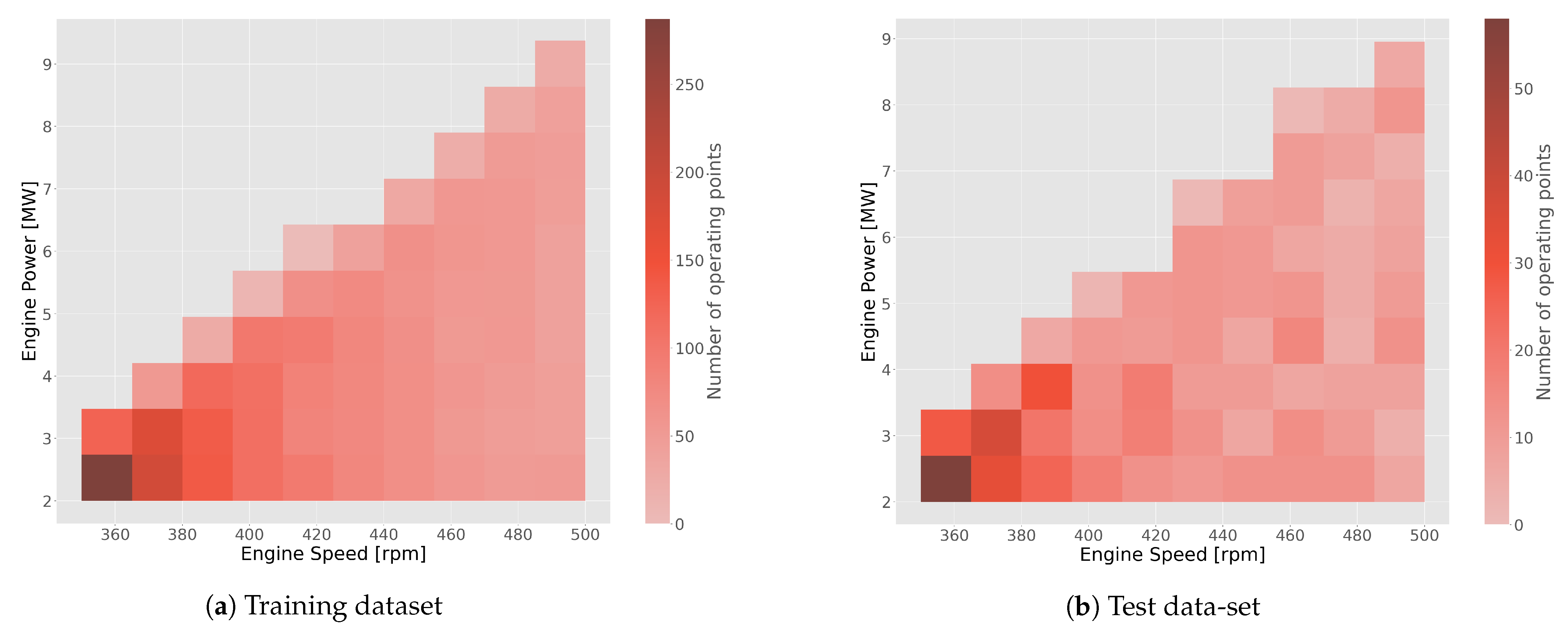
It must be noted that the distribution of testing datasets should be similar to the training datasets covering the complete engine operating envelope. Figure 2 presents the distribution of training and testing datasets for the considered marine engine operating envelope.

2.2. Feature Selection Approaches

Feature engineering involves the selection and transformation of input parameters for developing a machine learning regression model [20]. The commonly used wrapper approach [21] is employed in this case to identify the input parameters to develop a data-driven model for predicting in-cylinder pressure. It encompasses application of a suitable regression technique (ANN is used herein) with all the available input options.
This study considers the in-cylinder pressure prediction for healthy conditions. Therefore, the engine speed and power are considered independent parameters to represent the engine operating point. The fuel consumption (or injected fuel amount) becomes a dependent parameter, and hence is not employed as an input parameter.
However, since the output parameter (in-cylinder pressure) is a function of the crank angle (ranging 0–720 degrees for four-stroke engines), two approaches for developing data-driven models are considered. The first approach considers the estimation of the in-cylinder pressure with ANN regression, using engine speed, power, and crank angle as input for each cylinder. This approach can be represented using the following equation:
p ( α ) = f ( N e , P e , α ) n cyl
where N e , P e , n c y l are the engine speed, power and cylinder number, respectively, whereas α denotes the crank angle.
The second approach considers only the engine speed and power as input to derive the harmonics (Fourier series) coefficients via ANN regression. Subsequently, a block with a Fourier series function is employed to calculate the in-cylinder pressure by the following equation:
p ( α ) = A 0 + n = 1 N A n c o s 2 π n α T + n = 1 N B n s i n 2 π n α T
where coefficient A 0 denotes the average value of the in-cylinder pressure within the engine cycle; A n and B n coefficients represent the amplitudes of the cosine and sine functions of the n t h harmonic order; n denotes the individual coefficient number from 1 to N; N represents the total number of harmonics; T denotes the period of the periodic function (720 °CA).
The reference Fourier coefficients corresponding to the derived in-cylinder pressure datasets (Phase 1), which are termed C 1 , C 2 C 2 N + 1 henceforth, are also calculated in Phase 1 by using Fourier analysis [22], and mapped as functions of engine speed and power for each cylinder, i.e.,
( C 1 , C 2 C 2 N + 1 ) n c y l = f ( N e , P e ) n c y l
The number of harmonic orders required to accurately represent the in-cylinder pressure (with minimal error) depends on the pressure sampling rate (typically 1 °CA sampling requires 720 harmonic orders for four-stroke engines). However, for reducing dimensions for machine learning problems, fewer harmonic orders should be selected without losing meaningful information.
Therefore, 50 harmonic orders (N = 50) corresponding to 101 Fourier coefficients for each cylinder are selected herein for comparing the two approaches. This harmonics number is also employed for comparatively assessing the regression techniques described in Section 2.3.
A basic artificial neural network (ANN) for estimating the output parameters for the engine nine cylinders is employed for each approach. The details of the developed ANNs based on the first modelling approach is provided in Table 3. The input layer consists of three input parameters, specifically engine speed, engine power, and crank angle ( α ). The output layer has only one parameter for each cylinder, which is the in-cylinder pressure at a given crank angle ( α ). By iterating the crank angle values in the range 1–720°, the in-cylinder pressure within the complete engine cycle (for each engine cylinder) is calculated.
The second approach employs only two inputs (engine speed, and power) and estimates in total 101 outputs for each cylinder (909 for the engine nine cylinders), which include A N , B N and A 0 corresponding to 50 harmonic orders (N = 50). The in-cylinder pressure for each cylinder is then calculated in the pressure reconstruction block (Figure 1), by employing Equation (4) that uses these coefficients as input. The details of this approach ANN structure are provided in Table 4. The ’None’ in the model summary represents the variable batch size, as the employed software package does not consider fixed batch size by default.
The training of the two ANNs is carried out by using the training datasets selected as described in Section 2.1.2. The Adam optimiser [23] is used to reduce the root mean square error (RMSE) between the reference values y and the predicted values y ^ by using the backpropagation of the gradients over the hyperparameters determined in previous steps of the optimisation process. The Adam optimiser is able to adapt to new learning rates based on the number of steps required to reach the global minimum for RMSE.
The comparative assessment of the data-driven models based on these two approaches is presented in the results section, and demonstrates that the second approach is superior.

2.3. Data-Driven Models Based on Regression

This section focuses on the development and training of the data-driven models based on the second approach reported in Section 2.2 and six regression techniques. A parametric study is performed by using different training datasets for estimating these regression techniques’ accuracy.

2.3.1. Parametric Study

The available training datasets (4250 samples that were split from the generated datasets as reported in Section 2.1.2) are used to train the data-driven models. Further splitting of these datasets is carried out to select training datasets, by employing the split ratio ( γ ) calculated according to:
γ = 1 n Train n Train total
Only selected datasets from the total training datasets are used (by varying γ ) for training, allowing for the data-driven models’ accuracy assessment. This is achieved by using discrete values of γ ( γ = 0 implies that all the training datasets are used for training). Table 5 lists the γ values used for this parametric study. The data-driven models with the six regression techniques are trained using the training datasets corresponding to each γ value. The performance results of this parametric study are presented in the results section.
The following six regression techniques are employed to develop the data-driven models (second approach): linear regression, elastic regression, polynomial regression, support vector regression, decision tree regression, and artificial neural networks (ANN).

2.3.2. Multiple Linear Regression (LR)

Linear regression is one of the simplest machine learning techniques, which considers a linear combination of input parameters along with a bias ( θ 0 ) to to map the output [24]. To calculate the Fourier coefficients as a function of the engine speed and power, the following equation is employed:
C c y l = θ 0 , c y l + θ 1 , c y l N e + θ 2 , c y l P e
where C c y l = [ A 0 , A 1 , A N , B 1 , B N ] c y l and θ 1 , c y l , θ 2 , c y l   and   θ 3 , c y l are hyperparameters for each cylinder.
The loss function to minimise the prediction error is calculated by the following equation:
L = i = 1 n ( p ( α ) p ^ ( α ) ) 2
where p denotes the reference in-cylinder pressure, and p ^ denotes the in-cylinder pressure estimated from the data-driven model that uses the linear regression to predict the Fourier coefficients and the pressure reconstruction block (according to Equation (4)).

2.3.3. Elastic Regression (ER)

Elastic regression is a statistical modelling technique similar to linear regression that combines both L1 (Lasso) and L2 (Ridge) regularisation techniques to enhance the linear regression model’s performance and address potential issues like multicollinearity and overfitting [25]. It introduces a penalty term to the loss function, allowing for feature selection and reducing the impact of irrelevant features. The employed equation is similar to the linear regression on (Equation (7)).
However, the following equation is employed to calculate the loss function:
L = 1 2 n i = 1 n ( p ( α ) p ^ ( α ) ) 2 + λ 1 j = 1 2 | θ j | + λ 2 j = 1 2 ( θ j ) 2
where n is the number of training datasets; λ 1 and λ 2 denote the penalty terms for the L 1 and L 2 regularisations, respectively.

2.3.4. Polynomial Regression (PR)

Polynomial regression (PR) is a form of linear regression known as a special case of multiple linear regression. It maps the relationship between the input and output parameters as an nth degree polynomial [24]. Polynomial regression is sensitive to outliers, which greatly affect its accuracy. This study considers regression of second degree, employing the following equation for the estimation of the Fourier coefficients:
C c y l = θ 0 + θ 1 , c y l N e + θ 2 , c y l P e + θ 3 , c y l ( N e ) 2 + θ 3 , c y l ( P e ) 2 + θ 4 , c y l ( N e , P e )
where C c y l = [ A 0 , A 1 , A N , B 1 , B N ] c y l and θ 1 , c y l , θ 2 , c y l , θ 3 , c y l and θ 4 , c y l are hyperparameters for each cylinder.

2.3.5. Support Vector Regression (SVR)

Support vector regression (SVR) is a non-linear regression technique based on support vector machines (SVM) that approximates the provided dataset with a specific error margin [26]. It is used to identify a hyperplane that fits the training data whilst minimising error and maximising the distance from the hyperplane to support vectors (closest data points). SVR maps the input parameters to a higher-dimensional space using a kernel function.
SVR advantages include (a) versatility in handling linear and non-linear regression using different kernels (linear, polynomial, RBF, and sigmoid); (b) robustness with few samples or outlier data; (c) control over generalisation by using the margin parameter preventing overfitting; (d) effectiveness in high-dimensional spaces, rendering it suitable for datasets with high dimensions [27]. SVR disadvantages include (a) high computational effort for large datasets due to the use of quadratic optimisation; (b) challenges in selecting kernel and parameters; (c) lack of transparency due to complex kernels and reliance on support vectors [27].
Considering as input the engine speed and power, the SVR estimates the function f ( N e , P e ) i for the i t h Fourier coefficient by using the following equation:
( C c y l ) i ϵ f ( N e , P e ) i ( C c y l ) i + ϵ
where ϵ denotes the tolerance margin, whilst no penalty is considered to errors in the loss function minimisation. The settings for hyperparameters for the SVR regression are listed in Table 6.

2.3.6. Decision Tree Regression (DT)

Decision tree regression is a machine learning technique that develops a binary tree structure consisting of internal and leaf nodes to predict the regression tasks [28]. The internal nodes represent decisions based on features, whereas the leaf nodes provide the predicted output. The algorithm recursively splits the training data to minimise variance or maximise information gain. Predictions are made by traversing the tree from root to leaf. The standard settings for the model are described in the Table 6.
Decision trees’ advantages include (a) interpretability, providing a clear understanding of decision-making processes; (b) non-parametric structure, accommodating numerical and categorical features without assumptions on data distribution; (c) robustness to outliers due to relative ranking used in splitting; (d) representation of complex interactions and non-linear relationships among features [29]. Decision trees’ drawbacks include (a) overfitting if the tree depth or the number of features and relationships is uncontrolled; (b) sensitivity to slight changes in training data, leading to varying tree structures and predictions; (c) piece-wise constant predictions, lacking smoothness compared to other methods; (d) challenges when handling datasets with numerous irrelevant features [29].

2.3.7. Artificial Neural Networks (ANN)

Artificial neural networks (ANN) were inspired by biological nervous systems, and they are used to perform machine learning tasks including classification and regression. ANNs are extremely versatile as they can accurately model complex non-linear systems.
Multilayer perceptron (MLP) networks, which are also known as multilayer feedforward networks, are widely used in practical applications [30]. Two important parameters of MLP are the number of hidden layers and the number of neurons per layer (hidden layer size). The number of the hidden layers’ neurons is typically selected by using trial-and-error approaches to obtain the minimum converged squared error on the training data.

2.4. Metrics Selection

The developed data-driven models’ performance is evaluated based on the prediction of the in-cylinder pressure as well as the maximum cylinder pressure and the indicated mean effective pressure (MEP). The root mean square error (RMSE) of the predicted in-cylinder pressure for a complete engine cycle is calculated by using the following equation:
R M S E = i = 1 n ( p ( α ) p ^ ( α ) ) 2
where p ( α ) denotes the reference values of the in-cylinder pressure as a function of the crank angle ( α ) for each engine cylinder, whereas p ^ ( α ) represents the estimated in-cylinder pressure by the data-driven models. The accuracy of the given regression techniques is determined by the coefficient of determination ( R 2 ) considering the test (validation) datasets, which is calculated by the following equation:
R 2 = 1 i = 1 n ( p p ^ ) 2 i = 1 n ( p p ¯ ) 2
where i = 1 n ( p p ^ ) 2 is the sum of residuals and i = 1 n ( p p ¯ ) 2 is the total sum of squares (equal to variance) of the test datasets, with p ¯ denoting the mean value of pressure. In the best case, when the predicted values exactly match the reference values, R 2 becomes equal to 1.

3. Results and Discussion

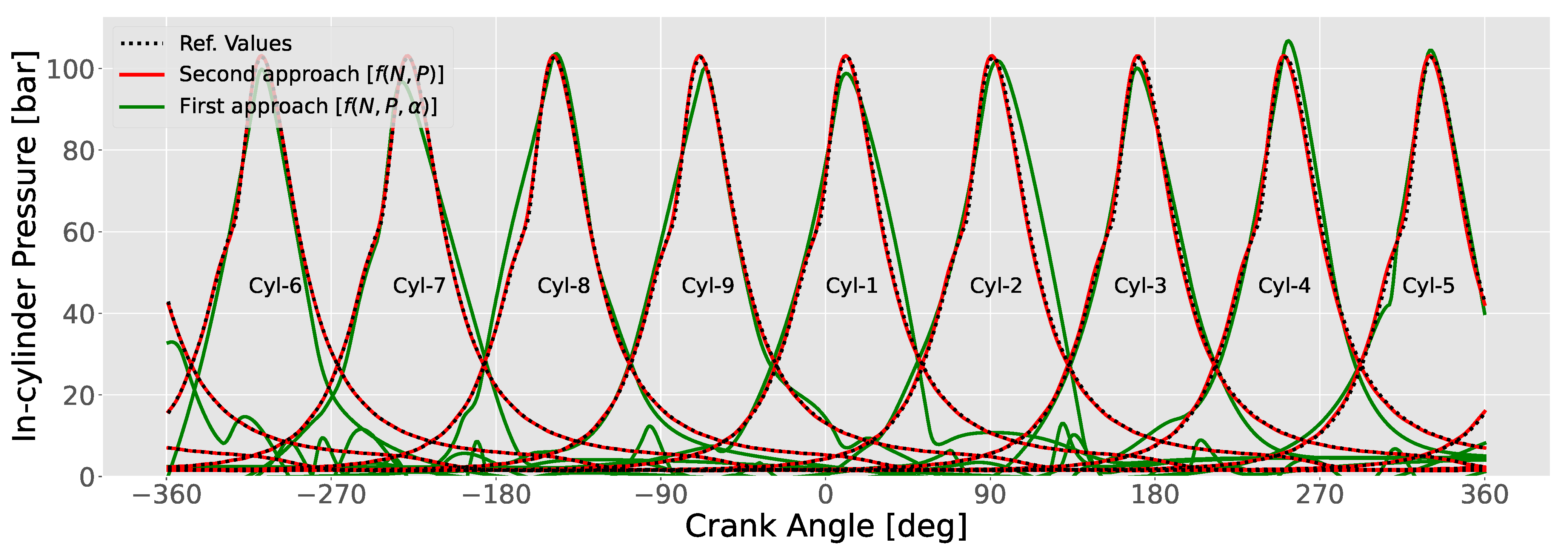
Figure 3 presents the predicted along with the reference in-cylinder pressure diagram for each engine cylinder for one engine cycle (crank angle from −360 °CA to 360 °CA) using the two approaches described in Phase 2 (Section 2.2). The dotted lines represent reference cylinder pressure (predictions of the thermodynamic digital twin), whereas the the green and red lines represent the predicted in-cylinder pressure by the first and second approach, respectively. It is inferred that the second approach provided in-cylinder pressure closer to the reference one (exhibiting a percentage error in the in-cylinder pressure prediction within ± 2 % ).
However, the first approach completely fails to predict the in-cylinder pressure at the open cycle. It provides adequate predictions for the closed cycle, although exhibiting higher errors compared to the predictions of the second approach. It is inferred that the first approach involves considerable errors, and does not satisfy the requirements of tools for marine engine health assessment. Therefore, the second approach, which involves the prediction of 101 Fourier coefficients per cylinder and subsequent reconstruction of the in-cylinder pressure by using Equation (4)), is selected for comparatively assessing the six regression techniques.
The data-driven models corresponding to the second approach and the six regression techniques are evaluated by using the test datasets ( 15 % of the total generated datasets), which were separated as reported in Section 2.1.2. The number of the test datasets corresponding to the several areas of the engine operating envelope are illustrated in Figure 2b.
The derived RMSEs (in bar, calculated according to Equation (13) considering the test datasets—750 samples) for the developed data-driven models corresponding to the six employed regression techniques, which were trained using training datasets derived by three different γ values (0.9, 0.95, and 0.995), are presented in Figure 4. The number of training samples for each γ value is listed in Table 5. It is deduced that the RMSE (for all regression techniques) increases with higher γ values, corresponding to smaller number training datasets. Therefore, a higher number of training datasets increases the data-driven model accuracy (lower RMSE). However, the RMSE changes for LR, PR, and ANN are not so pronounced, whereas RMSE values for gamma equal to 0.9 and 0.95 are almost the same. This implies the the Fourier series coefficients (second approach) can be effectively mapped using these linear regression techniques types, requiring a relatively low training dataset number. Contrary, the SVR and DT regression techniques are sensitive to γ and require higher dataset numbers. DT regression trained with the lowest datasets number exhibited low accuracy (high RMSE) on the test datasets. From the preceding discussion and presented results, it is inferred that the ANN regression is the most effective technique, as it resulted in RMSE less than 0.6 bar when trained using 20 datasets.
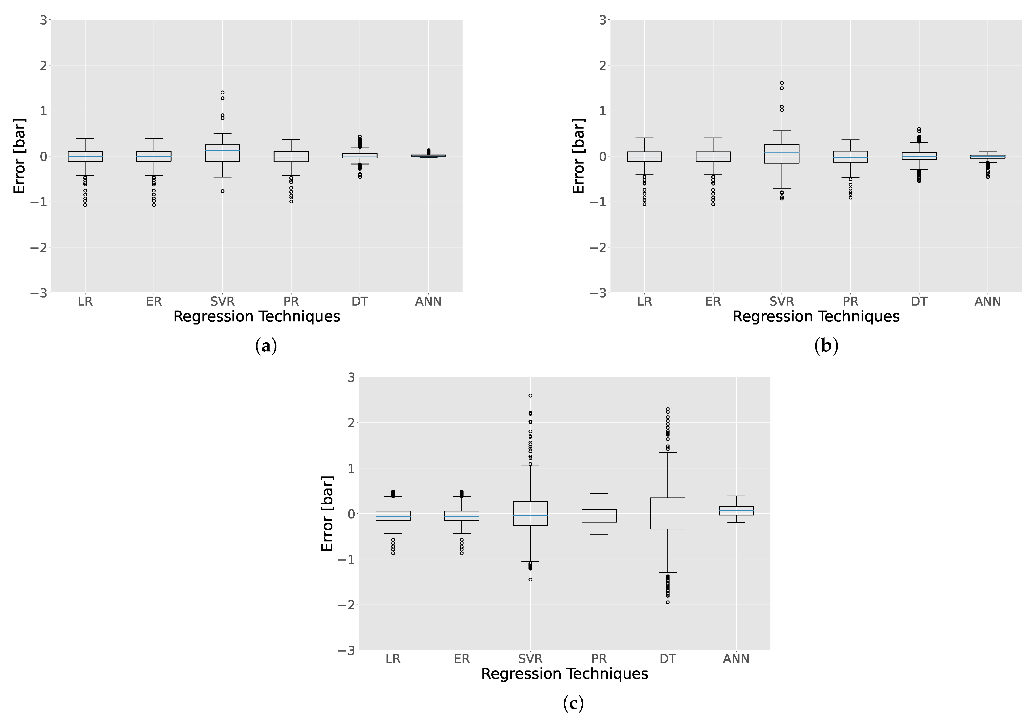
Figure 5 presents the average error of the predicted in-cylinder pressure (considering all the engine cylinders) by the data-driven models considering the test data (750 datasets); these data-driven models correspond to the six regression techniques trained using three different datasets ( γ = 0.9 , 0.95 , 0.995 ) . The range of the error distributions (whiskers) increases with the γ aligning with exhibited RMSE trends (Figure 4). The ANN regression exhibits an average error within ± 0.5 bar even when trained with the lowest dataset number. The DT regression performs adequately when trained using high numbers of training datasets. The ANN and PR regression techniques also showcase the minimum number of outlier error points with only 20 training samples. Therefore, it is deduced that the ANN and PR regression techniques exhibit the highest potential compared to the other regression techniques.
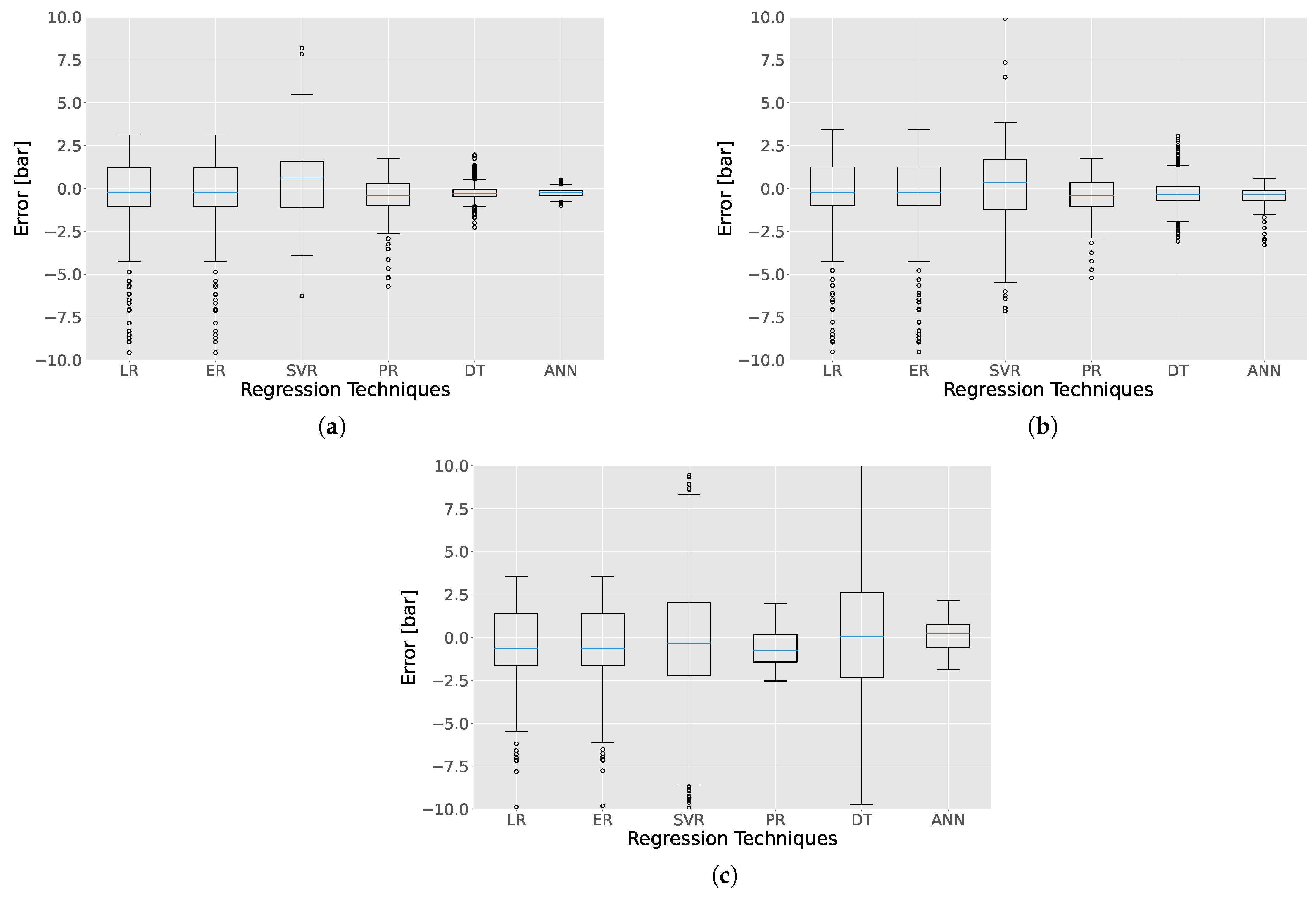
The predicted in-cylinder pressure diagrams (using the six regression techniques) are also used to derive other engine performance parameters, including the mean effective pressure (MEP) characterising the engine power output, and the in-cylinder maximum pressure ( p m a x ) characterising the engine thermo-mechanical limits. The accurate estimation of these parameters is important for marine engine health assessment. Figure 6 presents the average MEP error (from all the engine cylinders) considering the six regression techniques and the three γ values. The average MEP error remains almost the same for the linear regression techniques (LR, ER and PR) despite using different training datasets, which is in alignment with the respective RMSE trends of the in-cylinder pressure diagram prediction (discussed in the proceeding paragraphs). The SVR and DT techniques resulted in the highest MEP error variations. ANN use resulted in the lowest MEP errors, which gradually increased with the use of smaller training datasets. However, the ANN’s performance (considering the error tolerance and outliers) was found to be the best among all of the employed regression techniques. Positive offsets (mean of MEP errors) are observed for all the regression techniques, implying the MEP overestimation, which requires correction measures (e.g., the use of a negative bias).
Figure 7 presents the maximum in-cylinder pressure error (from all the engine cylinders) considering the six regression techniques and the three γ values. When using the highest training dataset number ( γ = 0.9 ), the ANN and DT regression techniques provided the lowest error distributions, whereas the respective mean errors exhibited slightly negative offsets. However, when using the lowest training dataset number ( γ = 0.995 ), the DT regression technique led to considerable errors, whereas the PR and ANN regression techniques resulted in errors ranging ± 2.5 bar. The PR regression led to mean errors with negative offset, the value of which increased with γ .
Figure 8 presents the absolute error of the predicted in-cylinder pressure from the data-driven models developed by the six regression techniques (and second approach) trained using 20 datasets ( γ = 0.995 ) on the whole engine operating envelope. These results are employed to characterise the ability of the employed regression techniques to predict the in-cylinder pressure throughout the investigated marine engine operating envelope. The data-driven models based on LR, ER, PR, and ANN regression techniques exhibited absolute error in predicting the in-cylinder pressure less than 1 bar considering the whole engine operating envelope. Data-driven models using the SVR and DT regression techniques exhibited higher absolute errors, reaching 4.8 and 2.4 bar, respectively, as shown in Figure 8c,e). The ANN regression exhibited the smallest absolute error compared to the other techniques in the whole operating envelope.
From the preceding discussion, it was confirmed that the the ANN regression exhibited the lowest errors in all the considered metrics considering the whole engine operating envelope, whilst requiring the smallest number of training datasets. Hence, the use of ANN regression is recommended for developing data-driven models to predict the marine engine in-cylinder pressure.
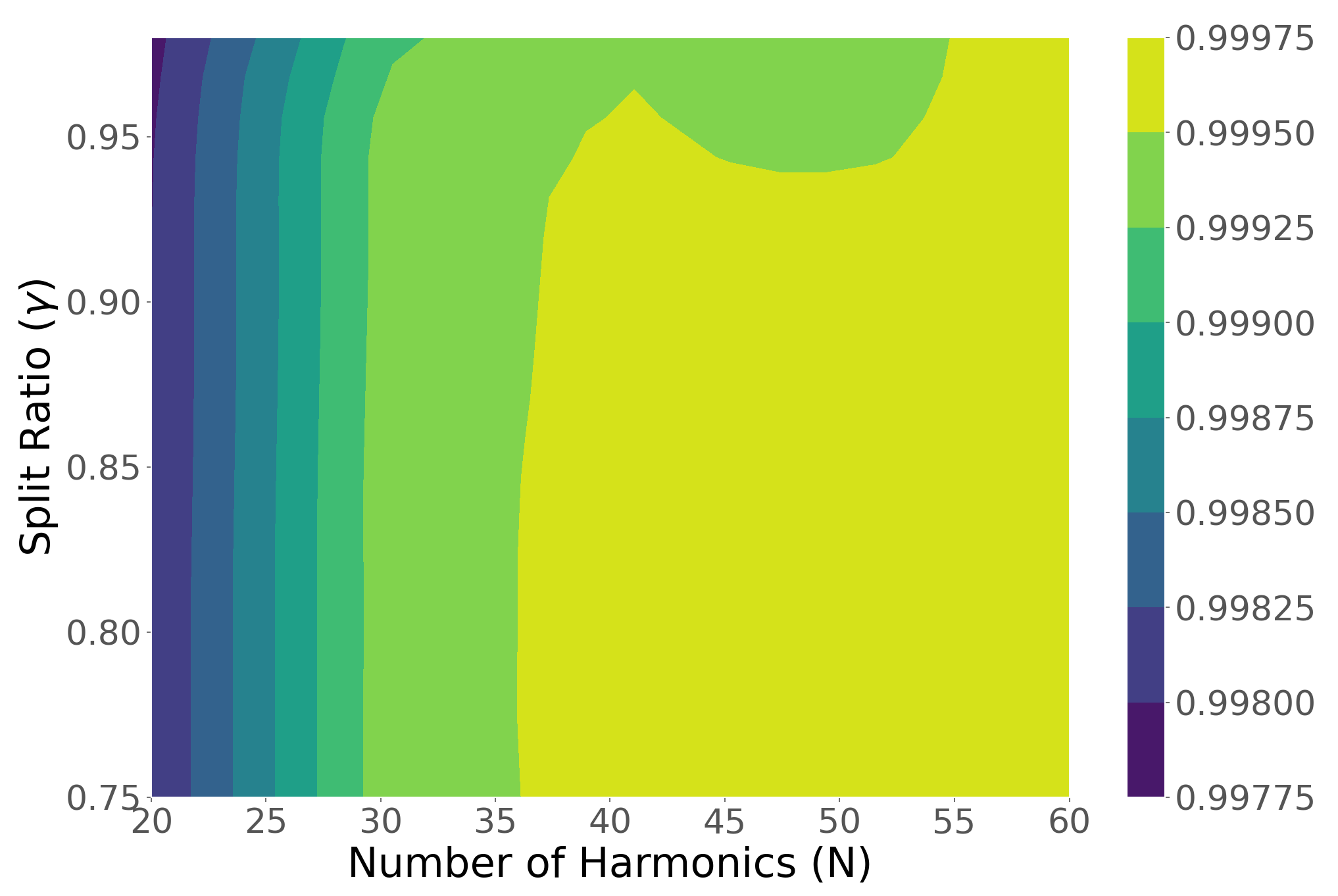
Figure 9 presents the results of the performed sensitivity study considering the data-driven model of the second approach and the ANN regression; the R 2 on the predicted in-cylinder pressure is plotted as function of the harmonics number (corresponding to 2 N + 1 Fourier coefficients for each cylinder) and test-to-train ratio ( γ , corresponding to the used training dataset number). It is deduced that the harmonic number greatly affects R 2 , which characterises the data-driven model error. For more than 45 harmonic orders, high R 2 values are observed, indicating sufficient accuracy. The test to train ratio slightly impacted R 2 . It is deduced that the proposed data-driven model using ANN regression trained with only 25% of the 4750 datasets (corresponding to engine operating points) randomly selected can achieve sufficient accuracy. This reduces the computational effort required for generating datasets (by employing the physical digital twins that are computationally expensive). The developed data-driven model can provide sufficient accuracy on the in-cylinder pressure prediction in healthy engine conditions, whilst substantially reducing the required computational effort.

4. Conclusions

This study comparatively assessed data-driven models for the in-cylinder pressure prediction of marine engines, which were developed based on two approaches and six regression techniques. The first approach employed as input for each cylinder the engine speed and power along with the crank angle to directly calculate the in-cylinder pressure via regression. The second approach employed as input the engine speed and power to calculate Fourier coefficients for each cylinder, which were subsequently used to calculate the in-cylinder pressure via the Fourier series function. The following regression techniques were employed: linear, elastic, and polynomial regression, support vector regression (SVR), decision trees (DT), and artificial neural networks (ANN). The main findings of this study are summarised as follows.
  • The second approach with ANN regression and 50 harmonics (corresponding to 101 Fourier coefficients per cylinder) was proved the most effective, exhibiting percentage errors for the in-cylinder pressure prediction within ± 2 % and RMSE within ± 0.2 bar when trained with only 20 datasets.
  • Simple linear regression techniques exhibited an overall root mean square error for the in-cylinder pressure prediction up to 0.65 bar with only 20 training samples.
  • ANN demonstrated the best performance on predicting the mean effective pressure and maximum in-cylinder pressure with minimum outliers compared to other methods.
  • A higher training dataset number led to higher accuracy of SVR, DT and ANN regression techniques, whereas linear regression techniques exhibited saturation in the predicted parameters error with the increase in the training dataset number.
  • The sensitivity study revealed that minimum 10 % of the training datasets (1000 samples) along with 45 harmonics led to RMSE values ranging 0.04–0.05 bar corresponding to R 2 ) close to 0.99 % .
  • ANN regression is therefore recommended for use in data-driven models for the prediction of marine engine in-cylinder pressure.
This study provided insights on the characteristics of regression techniques to develop data-driven models for marine engine performance parameter prediction. Future studies may consider more advanced regression techniques along with the extension of the operating envelope to include ambient and anomalous conditions. Heat release rate analysis of the in-cylinder pressure estimated by the data-driven model can also be investigated. Moreover, the prediction of other performance and emissions parameters can also be considered, thus moving forward to the establishment and validation of real-time, trustworthy digital twins for marine engines. The use of shipboard measurements to (re)train data-driven models as part of a prognostics framework is recommended.

Author Contributions

Conceptualization, C.P. and G.T.; methodology, C.P. and G.T.; software, C.P.; validation, G.T.; formal analysis, C.P. and G.T.; investigation, C.P. and G.T.; resources, C.P. and G.T.; data curation, C.P.; writing—original draft preparation, C.P. and G.T.; writing—review and editing, C.P. and G.T.; visualization, C.P.; supervision, G.T.; project administration, G.T.; funding acquisition, G.T. All authors have read and agreed to the published version of the manuscript.

Funding

This research was funded by Innovate UK, smart grants i-HEATS project, grant number 99958.

Data Availability Statement

Data sharing is not applicable to this article.

Acknowledgments

The authors greatly acknowledge the funding from DNV AS and RCCL for the MSRC establishment and operation. The opinions expressed herein are those of the authors and should not be construed to reflect the views of Innovate UK, DNV AS, and RCCL.

Conflicts of Interest

The authors declare no conflict of interest.

Nomenclature

N e Engine speed (rev/m)
nNumber of samples (-)
P e Engine power (kW)
pReference in-cylinder pressure (bar)
p ^ Predicted in-cylinder pressure (bar)
α Crank angle (°CA)
β Split ratio for separating test data (-)
γ Split ratio (-)
θ Hyperparameters (-)
μ Mean value of parameter (unit of parameter)
σ Standard deviation of parameter (unit of parameter)

References

  1. Mauro, F.; Kana, A. Digital twin for ship life-cycle: A critical systematic review. Ocean Eng. 2023, 269, 113479. [Google Scholar] [CrossRef]
  2. Coraddu, A.; Oneto, L.; Cipollini, F.; Kalikatzarakis, M.; Meijn, G.J.; Geertsma, R. Physical, data-driven and hybrid approaches to model engine exhaust gas temperatures in operational conditions. Ships Offshore Struct. 2022, 17, 1360–1381. [Google Scholar] [CrossRef]
  3. Mihai, S.; Yaqoob, M.; Hung, D.V.; Davis, W.; Towakel, P.; Raza, M.; Karamanoglu, M.; Barn, B.; Shetve, D.; Prasad, R.V.; et al. Digital twins: A survey on enabling technologies, challenges, trends and future prospects. IEEE Commun. Surv. Tutorials 2022, 24, 2255–2291. [Google Scholar] [CrossRef]
  4. Venkatesh, K.; Murugesan, S. Prediction of Engine Emissions using Linear Regression Algorithm in Machine Learning. Int. J. Innov. Technol. Explor. Eng. 2020, 9, 7. [Google Scholar] [CrossRef]
  5. Zhang, Y.; Wang, Q.; Chen, X.; Yan, Y.; Yang, R.; Liu, Z.T.; Fu, J. The Prediction of Spark-Ignition Engine Performance and Emissions Based on the SVR Algorithm. Processes 2022, 10, 312. [Google Scholar] [CrossRef]
  6. Alexiou, K.; Pariotis, E.G.; Leligou, H.C.; Zannis, T.C. Towards data-driven models in the prediction of ship performance (speed—power) in actual seas: A comparative study between modern approaches. Energies 2022, 15, 6094. [Google Scholar] [CrossRef]
  7. Liu, J.; Ulishney, C.; Dumitrescu, C.E. Application of Random Forest Machine Learning Models to Forecast Combustion Profile Parameters of a Natural Gas Spark Ignition Engine. Des. Syst. Complex. 2020, 6, V006T06A003. [Google Scholar]
  8. Yu, Z.J.; Haghighat, F.; Fung, B.C.M.; Yoshino, H. A decision tree method for building energy demand modeling. Energy Build. 2010, 42, 1637–1646. [Google Scholar] [CrossRef]
  9. Bhatt, A.N.; Shrivastava, N. Application of Artificial Neural Network for Internal Combustion Engines: A State of the Art Review. Arch. Comput. Methods Eng. 2022, 29, 897–919. [Google Scholar] [CrossRef]
  10. Wang, R.; Chen, H.; Guan, C. A self-supervised contrastive learning framework with the nearest neighbors matching for the fault diagnosis of marine machinery. Ocean Eng. 2023, 270, 113437. [Google Scholar] [CrossRef]
  11. Panda, J. Machine learning for naval architecture, ocean and marine engineering. J. Mar. Sci. Technol. 2023, 28, 1–26. [Google Scholar] [CrossRef]
  12. Noor, C.M.; Mamat, R.; Najafi, G.; Yasin, M.M.; Ihsan, C.; Noor, M. Prediction of marine diesel engine performance by using artificial neural network model. J. Mech. Eng. Sci. 2016, 10, 1917–1930. [Google Scholar] [CrossRef]
  13. Raptodimos, Y.; Lazakis, I. Application of NARX neural network for predicting marine engine performance parameters. Ships Offshore Struct. 2020, 15, 443–452. [Google Scholar] [CrossRef]
  14. Johnsson, R. Cylinder pressure reconstruction based on complex radial basis function networks from vibration and speed signals. Mech. Syst. Signal Process. 2006, 20, 1923–1940. [Google Scholar] [CrossRef]
  15. Saraswati, S.; Chand, S. Reconstruction of cylinder pressure for SI engine using recurrent neural network. Neural Comput. Appl. 2010, 19, 935–944. [Google Scholar] [CrossRef]
  16. Solmaz, O.; Gurbuz, H.; Karacor, M. Comparison of artificial neural network and fuzzy logic approaches for the prediction of in-cylinder pressure in a spark ignition engine. J. Dyn. Syst. Meas. Control. Trans. ASME 2020, 142, 091005. [Google Scholar] [CrossRef]
  17. Tsitsilonis, K.M.; Theotokatos, G. A novel method for in-cylinder pressure prediction using the engine instantaneous crankshaft torque. Proc. Inst. Mech. Eng. Part M: J. Eng. Marit. Environ. 2022, 236, 131–149. [Google Scholar] [CrossRef]
  18. Tsitsilonis, K.M.; Theotokatos, G.; Patil, C.; Coraddu, A. Health assessment framework of marine engines enabled by digital twins. Int. J. Engine Res. 2023, 24, 3264–3281. [Google Scholar] [CrossRef]
  19. Tsitsilonis, K.M.; Theotokatos, G. Engine malfunctioning conditions identification through instantaneous crankshaft torque measurement analysis. Appl. Sci. 2021, 11, 3522. [Google Scholar] [CrossRef]
  20. Khurana, U.; Samulowitz, H.; Turaga, D.S. Feature Engineering for Predictive Modeling using Reinforcement Learning. arXiv 2017, arXiv:1709.07150. [Google Scholar] [CrossRef]
  21. Maldonado, S.; Weber, R. A wrapper method for feature selection using Support Vector Machines. Inf. Sci. 2009, 179, 2208–2217. [Google Scholar] [CrossRef]
  22. Zeng, P.; Assanis, D.N. Cylinder Pressure Reconstruction and Its Application to Heat Transfer Analysis; SAE Technical Peper; SAE: Atlanta, GA, USA, 2004. [Google Scholar]
  23. Zhang, Z. Improved Adam Optimizer for Deep Neural Networks. In Proceedings of the 2018 IEEE/ACM 26th International Symposium on Quality of Service (IWQoS), Banff, AB, Canada, 4–6 June 2018; pp. 1–2. [Google Scholar]
  24. Bishop, C.M.; Nasrabadi, N.M. Pattern Recognition and Machine Learning; Springer: New York, NY, USA, 2006; Volume 4. [Google Scholar]
  25. Townsend, W. ELASTICREGRESS: Stata Module to Perform Elastic Net Regression, Lasso Regression, Ridge Regression; Research Papers in Economics; Boston College Department of Economics: Boston, MA, USA, 2017. [Google Scholar]
  26. Yang, X.S. Support vector machine and regression. In Introduction to Algorithms for Data Mining and Machine Learning; Academic Press: Cambridge, MA, USA, 2019. [Google Scholar]
  27. Basak, D.; Pal, S.; Patranabis, D.C. Support Vector Regression. Neural Inf. Process. Lett. Rev. 2007, 11, 203–224. [Google Scholar]
  28. Czajkowski, M.; Kretowski, M. The role of decision tree representation in regression problems—An evolutionary perspective. Appl. Soft Comput. 2016, 48, 458–475. [Google Scholar] [CrossRef]
  29. Loh, W.Y. Classification and regression trees. Wiley Interdiscip. Rev. Data Min. Knowl. Discov. 2011, 1, 14–23. [Google Scholar] [CrossRef]
  30. Szoplik, J. Forecasting of natural gas consumption with artificial neural networks. Energy 2015, 85, 208–220. [Google Scholar] [CrossRef]
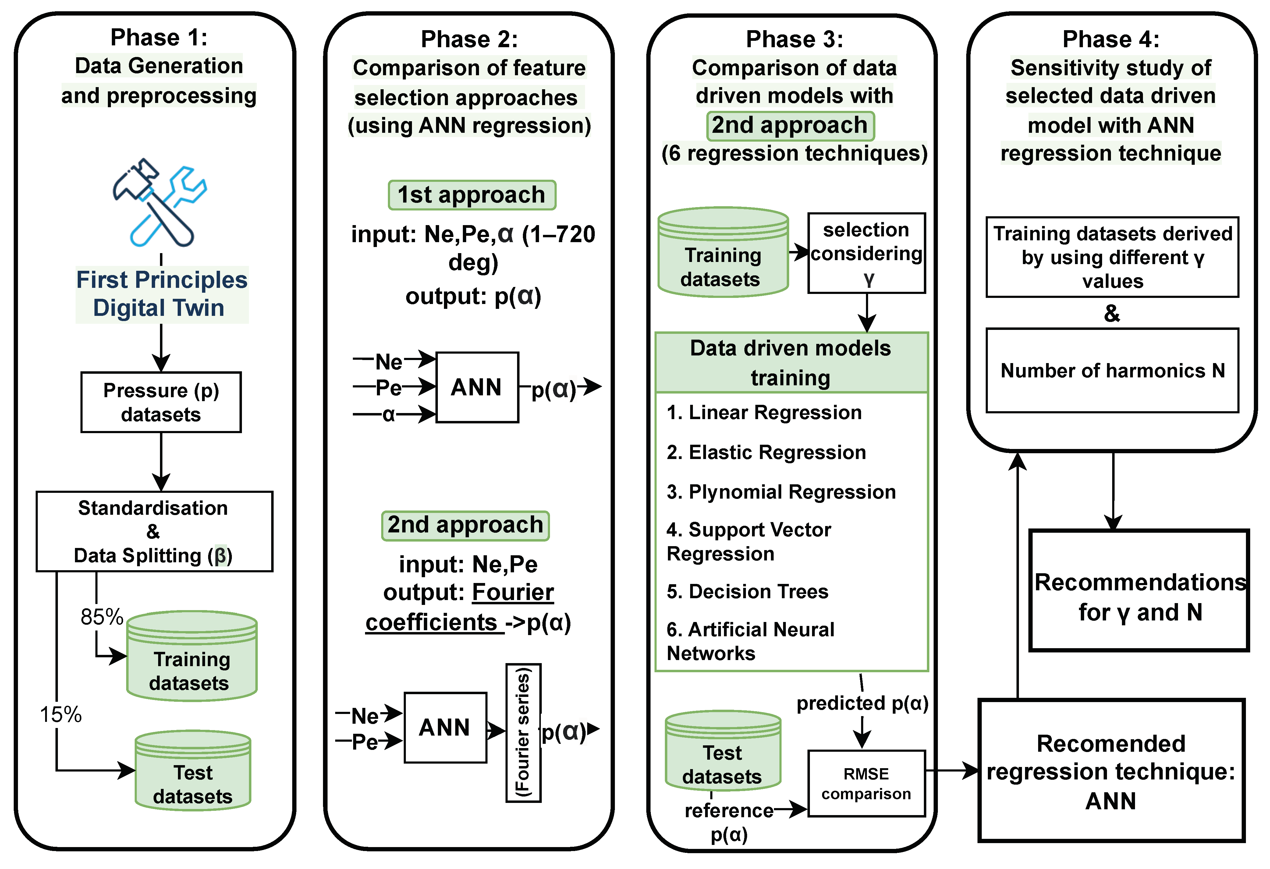
Figure 1. Methodology flowchart.
Machines 11 00926 g001
Figure 2. Distribution of operating points over the operating envelope of marine engine for training (a) and test (b) datasets selected by the splitting ratio β T e s t / T r a i n .
Machines 11 00926 g002
Figure 3. Predicted in-cylinder pressures using the data-driven model based on the first approach (green lines), the second approach (red lines), and reference values (dotted lines) for the engine operating point at 424 rpm and 3.06 MW.
Machines 11 00926 g003
Figure 4. Root mean square error for the six data-driven models (second approach and six regression techniques) for different training datasets (split using three values of γ ).
Machines 11 00926 g004
Figure 5. In-cylinder pressure error (average for 9 cylinders) of the data-driven models using six regression techniques and different γ values (0.9, 0.95, 0.995). (a) Training using 425 datasets ( γ = 0.9 ). (b) Training using 212 datasets ( γ = 0.95 ). (c) Training using 20 datasets ( γ   =   0.995 ).
Machines 11 00926 g005
Figure 6. Mean effective pressure (MEP) error (average for 9 cylinders) of the data-driven models using six regression techniques and different γ values (0.9, 0.95, 0.995). (a) Training using 425 datasets ( γ = 0.9 ). (b) Training using 212 datasets ( γ = 0.95 ). (c) Training using 20 datasets ( γ = 0.995 ).
Machines 11 00926 g006
Figure 7. Maximum in-cylinder pressure error (average for 9 cylinders) of the data-driven models using six regression techniques and different γ values (0.9, 0.95, 0.995). (a) Training using 425 datasets ( γ = 0.9 ). (b) Training using 212 datasets ( γ = 0.95 ). (c) Training using 20 datasets ( γ = 0.995 ).
Machines 11 00926 g007
Figure 8. In-cylinder pressure absolute error of data-driven models based on the six regression techniques and second approach trained using 20 datasets ( γ = 0.995 ) in the complete engine operating envelope.
Machines 11 00926 g008
Figure 9. Data-driven model based on the second approach and ANN regression– R 2 variation of the predicted in-cylinder pressure against the harmonics number and γ .
Machines 11 00926 g009
Table 1. Reference marine engine technical specifications.
Maximum Continuous Rating (MCR) power9450 kW
MCR speed500 rpm
Cylinders No.9
Cylinder Bore460 mm
TurbochargerABB TPL 77-A30
Table 2. Digital twin validation results at healthy conditions; adapted from [18].
Operating PointBSFC (% error) p max (% error)
4.725 MW @ 500 RPM2.72.5
7.088 MW @ 500 RPM1.23.0
8.033 MW @ 500 RPM–0.10.0
9.450 MW @ 500 RPM–0.5–0.4
1.0395 MW @ 500 RPM–1.2–0.1
6.143 MW @ 440 RPM1.041.2
4.725 MW @ 400 RPM0.10.1
Table 3. ANN regression characteristics—first approach.
Layer (Type)Output ShapeParameters
Input layer(None, 4)0
Hidden layer (dense)(None, 10)50
Hidden layer (dense)(None, 10)110
Output layer(None, 1)11
Table 4. ANN regression characteristics—second approach.
Layer (Type)Output ShapeParameters
Input layer(None, 3)0
Hidden layer (dense)(None, 10)30
Hidden layer (dense)(None, 10)110
Output layer(None, 909)999
Table 5. Parametric study of training datasets’ split ratio ( γ ) to select training datasets for the developed data-driven models.
Split Ratio ( γ )Training Datasets PercentageTraining Datasets Number
0.910%425
0.955%212
0.9950.5%20
Table 6. Hyperparameter settings and error minimisation criteria for the employed regression techniques.
Regression TechniqueAbr.Error MinimisationHyperparameters
Multiple Linear RegressionLRMean Squared Error
Elastic RegressionERMean Squared Error
Polynomial RegressionPRMean Squared ErrorDegrees: 2
Support Vector RegressionSVRMean Squared ErrorKernel: ’rbf’
D e g r e e = 3
C = 1 1
ϵ = 0.1 2
Γ = 1 / ( n o . f e a t u r e s × X . v a r ( ) ) 3
Decision Tree RegressionDTMean Squared ErrorSplitter: ’best’
minimum sample split: 2
Artificial Neural NetworksANNMean Squared ErrorHidden layers No: 2 (exponential linear unit activation)
Output layers No: 1 (linear activation)
Neurons No per hidden layer: 10
Epochs No: 200
1 C: Regularisation parameter. 2  ϵ : Epsilon SVR model. 3 Γ : Kernel coefficient.
Disclaimer/Publisher’s Note: The statements, opinions and data contained in all publications are solely those of the individual author(s) and contributor(s) and not of MDPI and/or the editor(s). MDPI and/or the editor(s) disclaim responsibility for any injury to people or property resulting from any ideas, methods, instructions or products referred to in the content.