Dimensional Error Prediction of Grinding Process Based on Bagging–GA–ELM with Robust Analysis

Abstract

Grinding, which determines the final dimension of parts, is an important process in manufacturing companies. In praxis, in order to avoid quality problems on the customer’s side, an online dimension check is normally used after the grinding process to ensure the product dimensions; however, it is always hysteretic and needs extra space and machine investment. To deal with the issue, dimensional error prediction of the grinding process is highly needed, and does not require extra space or machinery, as well as having better real-time performance. In this paper, a dimensional error prediction algorithm using principal component analysis (PCA), extreme learning machine (ELM), genetic algorithm (GA), and ensemble strategy (bagging algorithm) is designed. Specifically, PCA is used as a pre-treatment method to extract the main relevant components, then a bagging–GA–ELM model is constructed to predict the final product dimensional error after the grinding process, in which extreme learning machine (ELM) is utilized as a basic framework because of its fast calculation speed. GA, with its excellent global optimization capability, is implemented to search optimal input weights and thresholds of ELM, enabling ELM to obtain a better prediction performance. In addition, considering the complex environment of the industrial field, the bagging algorithm is employed to enhance the anti-noise ability of the proposed algorithm. Finally, the proposed algorithm is verified by a case from a bearing company.

1. Introduction

Grinding is a vital manufacturing process, which has a significant impact on a final part’s surface quality and cost [1]. With the increasing competition in manufacturing industries, the pursuit of higher quality and lower costs puts the focus on the grinding process. [2,3,4]. In fact, the grinding process is complex and the final quality and cost are highly related to the process parameters; therefore, many researchers study the influence of the process parameters on quality and cost. Then, artificial intelligence (AI) techniques are used to optimize process parameters to improve product quality and process efficiency [5,6]. In the literature [7], an improved differential evolution algorithm (DE) based on double populations is employed to optimize the grinding operation, and, finally, the surface roughness is effectively reduced. Mondal et al. [8] use particle swarm optimization (PSO) to find the optimal parameters for minimizing the surface roughness of a crane-hook-pin in the grinding process. Furthermore, in order to obtain faster convergence speed and higher performance of models, the idea of a multi-algorithm fusion-based technique has gained a lot of attention in recent years [9,10,11,12]. Huang et al. [13] utilize the Taguchi method and grey relational analysis (GRA) to obtain the optimal parameters in the cylindrical grinding process, which successfully solves the problem of minimizing surface roughness and maximizing material removal rate.

On the other side, in practice, a quality check is usually used to avoid quality problems on the customer’s side. Currently, the majority of quality checking operates offline, which increases the production throughput time and furthers quality risks. In addition, it also makes the process difficult to trace. Therefore, to reduce grinding cost and increase process control ability, many researchers focus on online quality checks and online quality predictions based on data collected in real-time [14,15,16].

However, an online quality check requires enterprises to provide extra space and investment. Moreover, the online quality check is always hysteretic; when a quality problem is detected, some further products which are already produced and in the transmission facility (conveyor, Truss manipulator), are already affected. Compared to online quality checks, online quality prediction does not need further space or equipment, and it also has the advantage of instantaneity. Once the quality problem is predicted based on real-time collected data and a prediction algorithm, the process can be stopped to avoid further loss. Therefore, online quality prediction has become a hot topic. Chen et al. [17] propose a novel acoustic signal-based detection method by combining a random forest algorithm (RF) and multiple linear regression model (MLR); at the end, the online prediction problem of tool wear in the grinding process is successfully solved. Li et al. [18] adopt a multi-scale attention convolutional neural network (CNN) to predict the final machining quality of the workpiece. It finally shows the high accuracy of online prediction of the material removal state in experiments.

Recently, researchers also tend to use neural networks with a more complex structure to obtain better prediction accuracy [19,20]. Guo et al. [21] present a novel online prediction system of surface roughness in the grinding process by combining the long short-term memory (LSTM) network with a hybrid feature selection approach; ultimately, it shows good prediction performance. Yin et al. [22] propose a reliable prediction model based on a genetic algorithm (GA) and deep neural network (DNN), and prove its feasibility in the prediction of the roughness and subsurface material damage in the real-time grinding process. However, it also should be noticed that, although the complex neuron network increases the accuracy of prediction, it also makes a significant reduction in calculation efficiency, which has difficulty meeting the requirements of high calculation efficiency in online quality prediction.

Extreme learning machine (ELM) [23] has received more attention for high computational speed and global approximation capability [24]. However, during the prediction process of ELM, some network parameters are determined randomly, which causes the fluctuation of prediction performance and also will lead to an accuracy reduction of product dimensional error prediction. Thus, the fusion of ELM and a heuristic algorithm is needed in order to obtain better prediction performance [25,26,27]. Liu et al. [28] propose a multi-kernels fault diagnostic model based on ELM and PSO; the suggested fault diagnostic model is tested by well-known rolling bearing data set and achieves successful identification of bearing faults. Sun et al. [29] obtain a prediction model of the extrusion grinding process by combining the ELM model with GA (GA–ELM), based on the comparison results of experiments, the GA–ELM model keeps the actual data prediction error within ±4%. However, compared to GA, although the reason for the faster convergence speed of PSO is that the best particles have a significant influence on other particles, it also causes the problem of poor population diversity, which limits the PSO to obtain the global optimum. Therefore, GA has a better ability to acheive a globally optimal solution [30,31,32,33].

Moreover, as is well known, in a real industrial environment, the random interference and noise from various processes as well as environments have a non-negligible impact on the online prediction results. For ensuring the reliability of prediction results, it is necessary to improve the robustness of the prediction approach. Currently, the ensemble learning algorithms represented by bagging and boosting have been widely verified because of their ability to improve the accuracy and stability of prediction [34], Gao et al. [35] propose a novel material removal model for belt grinding with the integration of a boosting algorithm, which shows an effective improvement in predicting the material removal despite the complicated grinding environment. Bustillo et al. [36] verify the effectiveness of the bagging algorithm in the case of tool-life prediction in the turning process. The experiments show that the technique of bagging significantly improves the robustness of the prediction model. Furthermore, it should be noted that the bagging algorithm has the characteristics of simple operation, strong interpretability, and excellent performance. In general, the bagging algorithm has more obvious benefits than the boosting algorithm in preventing the overfitting problem and improving the noise immunity of the model [37,38]. Thus, the bagging algorithm is employed to improve the robustness of the proposed algorithm.

As mentioned above, considering the complex environment and processing property, to predict the grinding dimensional error, it is necessary to introduce an algorithm with excellent global search ability, fast calculation speed, high prediction accuracy, and good robustness. Therefore, a dimensional error prediction algorithm which combines the advantages of ELM, GA, and bagging algorithm, is proposed.

2. Materials and Methods

In this section, the theoretical background of the proposed algorithm is introduced first, which consists of PCA, GA, ELM, and bagging algorithm. Then, the proposed algorithm is explained in detail.

2.1. Principal Component Analysis

In order to improve the accuracy and robustness of the proposed algorithm, the feature parameters which are related to the final product dimension should be regarded as inputs of the proposed algorithm. Considering that excessive feature parameters will lead to a calculation efficiency reduction as well as the overlap of information, it is necessary to further extract the main relevant components from feature parameters to simplify the inputs of the proposed algorithm.

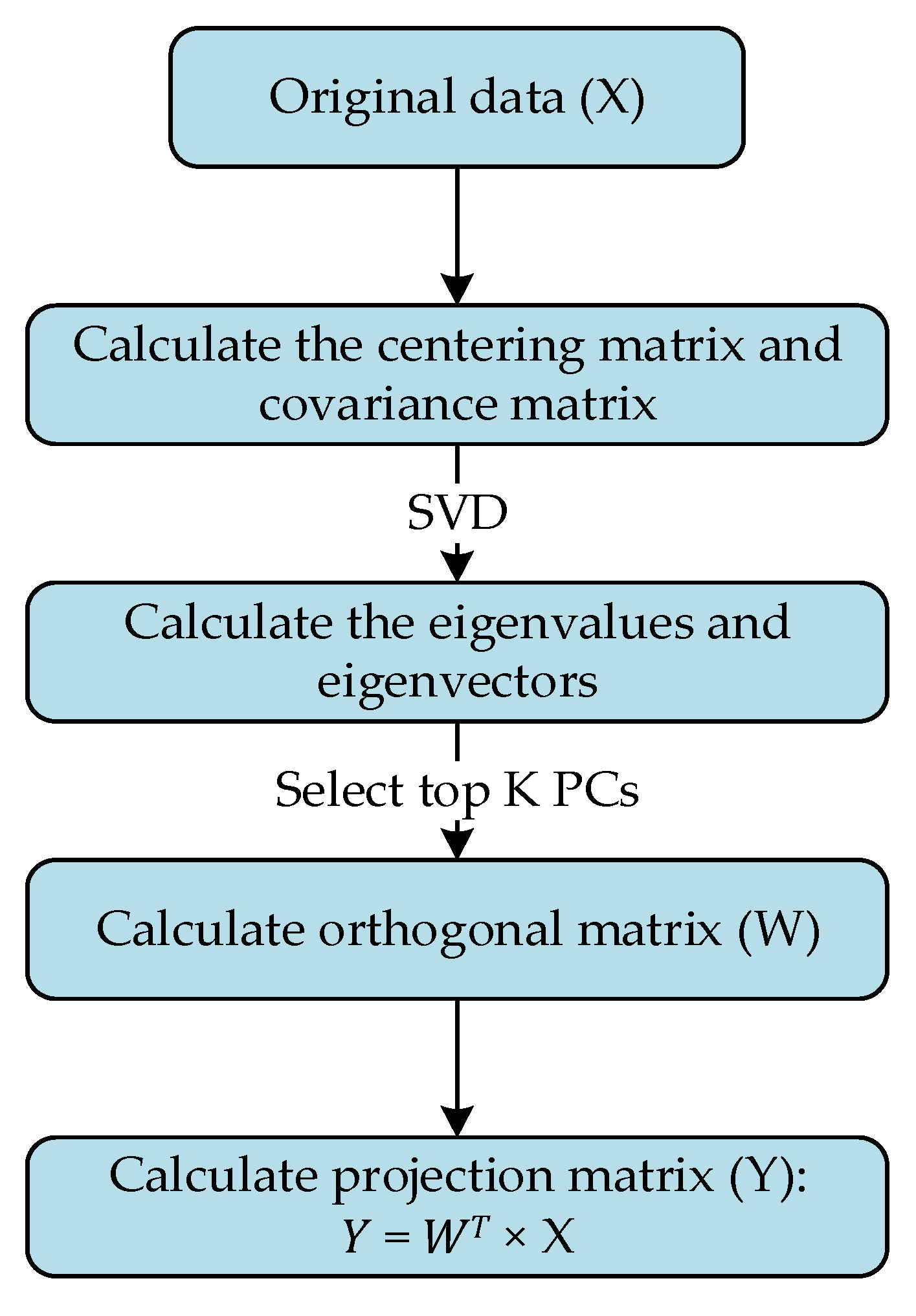
Principal component analysis (PCA) [39] is a technique used for reducing the dimension of data, which is widely employed in the analysis of the machining process for removing redundant variables and extracting the main relevant components. The calculation process of PCA is shown in Figure 1 and defined as follows:

Step 1. Suppose original data, named X, consists of N samples with D dimensional features; the centering matrix of original data is given by Equation (1) and the covariance matrix can be further calculated by Equation (2).

Step 2. Via singular value decomposition (SVD), the principal components (PCs) consist of eigenvalues, and eigenvectors are computed from the eigen-decomposition operation of the covariance matrix, which is shown in Equation (3).

Step 3. K (lower than D) eigenvectors are usually picked out to form the orthogonal matrix (W). For this aim, the conventional methodology is used to sort the eigenvalues from maximum to minimum and to select the top K PCs. Finally, the projection matrix Y can be calculated as $Y=W^T\times X$.

$$X_c={{\displaystyle \sum }}_{i=1}^N\left(x_i-\overline{X}\right)/N$$

(1)

$$C=X_c\times X_c{}^T$$

(2)

$$C=V\times E\times V^T$$

(3)

where $\overline{X}$ and $X_c$ are the mean vector and centering matrix of original data, respectively, $C$ denotes the covariance matrix, $V$ and $E$ represent the eigenvalue matrix and eigenvector matrix, respectively.

2.2. Extreme Learning Machine

Due to the characteristics of simple structure, fast calculation speed, and excellent ability in the field of prediction, an extreme learning machine (ELM) [23] is taken as the basic framework of the proposed algorithm.

ELM is a new type of single hidden layer feed-forward neural network (SLFN). The neural network structure of ELM has only three network layers namely the input layer, the hidden layer, and the output layers. The schematic diagram of ELM is shown in Figure 2, and the ELM model can be established as follows:

Firstly, the network parameters of the ELM model should be determined. According to Figure 2, the network parameters mainly consist of the input weights (W), output weights ($\beta$) and the threshold of the hidden neuron (b), as shown in Equation (4). The determination of network parameters is introduced by two steps:

Step 1. The input weights and the threshold of the hidden neuron are given randomly;

Step 2. The output weights are obtained by solving the least squares solution of the ELM, which is shown in Equations (5)–(7).

Secondly, based on the determined network parameters, the prediction results can be obtained by Equation (8).

$$W=\left[\begin{array}{ccc}{w}_{11}& \cdots & w_{1p}\\ ⋮& \ddots & ⋮\\ w_{d1}& \cdots & w_{dp}\end{array}\right], \beta =\left[\begin{array}{ccc}{\beta }_{11}& \cdots & {\beta }_{1q}\\ ⋮& \ddots & ⋮\\ {\beta }_{p1}& \cdots & {\beta }_{pq}\end{array}\right], b={\left[\begin{array}{ccc}{b}_1& \cdots & b_p\end{array}\right]}^T$$

(4)

$$X={\left[\begin{array}{ccc}{x}_1& \cdots & x_d\end{array}\right]}^T, Y={\left[\begin{array}{ccc}{y}_1& \cdots & y_q\end{array}\right]}^T$$

(5)

$$O=g\left(X^{T}W+b^T\right)$$

(6)

$$\beta ={\left(O^{T}O\right)}^{-1}{O}^T{Y}^T$$

(7)

$$Y_{pre}=g\left(X^{T}W+b^T\right)\beta$$

(8)

where $w_{ij}$ denotes the connection weight of i-th neuron of the input layer and the j-th neuron of the hidden layer, ${\beta }_{jm}$ denotes the connection weight of j-th neuron of the hidden layer and the m-th neuron of the output layer, $b_k$ denotes the threshold of k-th hidden neuron, $X$ and $Y$ are the input and output data of ELM model, $W$, $b$, $\beta$, $g\left(·\right)$, and $O$ represent input weight matrix, threshold matrix, output weight matrix, activation function and output matrix of hidden layer, respectively.

2.3. Genetic Algorithm

Because some network parameters (input weights and threshold) of ELM are determined randomly, this leads to the fluctuation of prediction performance. In order to achieve stable prediction performance and high prediction accuracy, it is necessary to combine the ELM model with another algorithm with excellent global optimization ability.

Based on the selection operation, crossover operation, and mutation operation, the genetic algorithm (GA) [40] can keep the population diversity effectively to avoid the local optimal solution, so that it has a global optimization capability [27,41]. Thus, GA is employed to optimize the ELM by globally searching the optimal value of input weights as well as a threshold in this research, and the flow of GA is shown in Figure 3 and defined as follows:

Step 1. The parameters of GA are determined at first, which consists of the chromosome number in the population, the maximum generation, crossover rate, and mutation rate.

Step 2. Then, the variables of non-linear problems are encoded as the chromosome for obtaining the primary population.

Step 3. Subsequently, the fitness value of each chromosome will be calculated as an evaluation method. By simulating the survival of the fittest in the biological evolution process, the chromosomes with higher fitness value have more possibility to be selected into the next generation and the others will be dropped. The formula is shown in Equation (9).

Step 4. In addition, so as to increase the diversity of the population, crossover operation and mutation operation are necessary. In addition, it is essential to increase the diversity of the population, crossover operation, and mutation operation. The former will randomly select several pairs of chromosomes for crossover based on the crossover rate, which is shown in Equation (10). Furthermore, as shown in Equations (11) and (12), the latter will make the genes of each chromosome mutate by the mutation rate.

Step 5. Finally, repeat step 3 and step 4 until meeting the termination condition. The chromosome with the highest fitness value will be regarded as the best solution to non-linear problems and decoded as the value of related parameters.

$$P_i=f_i/{{\displaystyle \sum }}_{j=1}^M{f}_j$$

(9)

$$Z_1^{t+1}=\phi \times Z_1^t+\left(1-\phi \right)\times Z_2^t, Z_2^{t+1}=Z_1^t+\phi \times \left(Z_1^t+Z_2^t\right)$$

(10)

$$\mathrm{∆}\left(t,z\right)=z\times \theta \times {\left(1-t/T\right)}^b$$

(11)

$$z^{t+1}=\{\begin{array}{c}{z}^t+\mathrm{∆}\left(t,\left(1-z^t\right)\right), \theta >0.5\\ z^t-\mathrm{∆}\left(t,\left(z^t+1\right)\right), \theta \le 0.5\end{array}$$

(12)

where $f_i$ and $P_i$ denote the fitness value and selection probability of i-th chromosome, respectively, $Z_1^t$ and $Z_2^t$ represent the pair of chromosomes in t-th generation, $\phi$ and $\theta$ are random values between 0 and 1, $T$ is the value of the maximum generation, $z^t$ denotes a gene in t-th generation.

2.4. Bagging Algorithm

Since the various environmental noise is inevitable and it will greatly influence the final prediction result, therefore, the anti-interference ability of the proposed algorithm needs to be focused. The bagging algorithm [42] is a widely used ensemble strategy. By constructing several base learners and combining the outputs of base learners to obtain a comprehensive evaluation, the bagging algorithm has a powerful ability to solve overfitting problems with the characteristics of high variance. Thus, the bagging algorithm will be utilized as the further optimization algorithm to prevent overfitting problems as well as improve the generalization and robustness of the prediction process.

The mechanism of the bagging algorithm is shown in Figure 4 and illustrated as follows:

Step 1. The bootstrap sampling method is used to obtain several training subsets from the training set, which adopts the strategy of random sampling with replacement.

Step 2. Then, each base learner will be trained by the corresponding training subsets.

Step 3. The multiple prediction results will be generated by base learners and combined to form an aggregated output.

2.5. Proposed Dimensional Error Prediction Algorithm

In order to solve the problem of dimension prediction in the grinding process, a dimensional error prediction approach with the advantages of fast calculation speed, high accuracy, and strong robustness is proposed.

The main idea of the proposed algorithm can be divided into two parts: the raw data is pre-treated at first to remove the redundant information as well as noise. Next, the bagging–GA–ELM algorithm will rapidly learn the complex mapping between parameters and dimensional error to obtain excellent prediction performance, in which the ELM model is taken as a basic framework at first, then it is optimized by the GA to obtain the optimal network parameters. Finally, the bagging algorithm is utilized as further optimization to improve the robustness of ELM model.

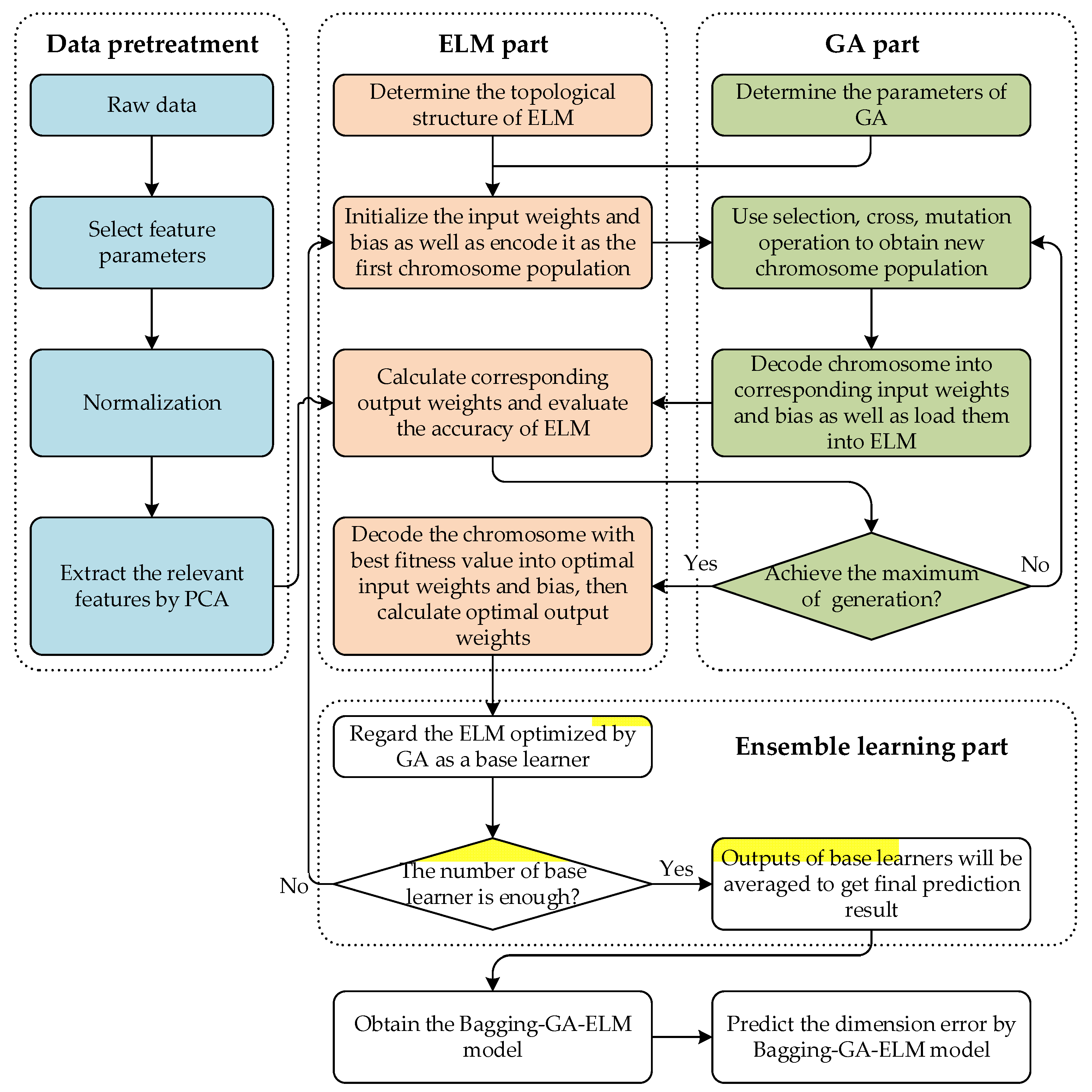
The block diagram of proposed algorithm is shown in Figure 5 and described as follows:

Firstly, for obtaining the bagging–GA–ELM model with higher accuracy and robustness, the raw data should be pretreated, which contains three aspects:

• In the grinding process, some process parameters have a significant impact on the final product dimension, and it also has an obvious influence on the final prediction performance of bagging–GA–ELM [43,44]. Therefore, relevant parameters which are chosen by processing property, previous experiments, and relevant theories, are selected as feature parameters, such as the grinding power of the fine grinding process, the grinding power of the spark out process, etc.
• Then, normalization is used to eliminate the difference of dimension among different parameters, and PCA is used to extract the main-relevant components from feature parameters. Both of them can improve the calculation speed of the bagging–GA–ELM model. Especially, the negative noise can be avoided by using PCA.
• At last, the training set is divided into different training subsets by the strategy of random sampling with replacement, which aims to provide the foundation for the subsequent ensemble learning optimization.

Secondly, the bagging–GA–ELM is proposed to predict dimensional error as well as to avoid the scrap with a dimension problem flowing to the customer. The proposed bagging–GA–ELM model consists of the following three parts:

• ELM is used as a basic framework to predict dimensional error because of its fast calculation speed and excellent ability in the field of industrial prediction. Although ELM just uses the single hidden layer feed-forward network structure, it can also achieve good prediction performance with high accuracy by increasing the width of the network (the number of hidden layer neurons) [45,46]. In addition, compared with other complex neural networks, especially deep neural networks, the design of a single hidden layer greatly reduces the size of network parameters, which makes ELM obtain extremely high calculation efficiency. Hence, the ELM model is selected in this research to learn the nonlinear relationship between selected features and the dimensional error;
• The optimization of ELM with GA: the traditional ELM model is characterized by short training time, high execution efficiency, and strong generalization ability. However, because some network parameters (input weights and threshold) of ELM are determined randomly, this results in the fluctuation problem of prediction performance. Therefore, the GA which has global optimization capability, is combined with ELM to search the optimal network parameters, and the optimization detail is delineated as follows:

Step 1. The encoding process of chromosomes: each network parameter (input weight and threshold) will be encoded as a gene and aligned in a row, namely chromosomes. Then, based on the random determination of network parameters, different values of parameters generate different chromosomes until meeting the size of the population.

Step 2. Evaluation of chromosomes: via loading network parameters carried by the chromosome into the GA–ELM part, the prediction accuracy of the training set is used to calculate the fitness value of the chromosome. The formulas are shown in Equation (13).

Step 3. The decoding process of chromosomes: based on the optimization of the GA part, the chromosome with the best fitness value will be decoded into network parameters according to the reverse operation of the encoding process. Then, in accordance with the training set, the output weights will be further decided by solving the least squares solution of the ELM part. Finally, the prediction function of the GA–ELM part is shown in Equation (14).

$$f_i=exp\left(-\sqrt{{{\displaystyle \sum }}_{k=1}^N\left(y_k-{\widehat{y}}_k\right)/N}\right)$$

(13)

$$Y_{pre}={\beta }^{T}g\left(W^{T}X+b\right)$$

(14)

where $f_i$ denotes the fitness value of i-th chromosome, $y_k$ and ${\widehat{y}}_k$ represent the observed value and predicted value of k-th sample, $N$ denotes the sample number, $W$, $b$, $\beta$ and $g\left(·\right)$ represent input weight matrix, threshold matrix, output weight matrix and activation function of ELM part, respectively, $X$ and $Y_{pre}$ are matrices of parameters and prediction values of dimensional error, respectively.

3.

The improvement of prediction robustness by bagging algorithm: due to the unavoidable environmental noise in the real grinding process, which will greatly influence the final prediction result, it is important to ensure the robustness of the proposed algorithm. Since the bagging algorithm has the characteristics of simple operation, strong interpretability, and excellent performance, and it also has significant advantages in preventing the overfitting problem and improving the anti-noise ability of the model, thus, the bagging algorithm is employed to improve the robustness of the proposed algorithm. Based on the bootstrap sampling method, the bagging–GA–ELM model is formed by the base learners trained from different training sets, and the output of bagging–GA–ELM is obtained by averaging the outputs of base learners.

Finally, the bagging–GA–ELM will be obtained and used in the prediction of dimensional error with high accuracy and strong robustness.

3. Results

For proving the feasibility and effectiveness of the proposed algorithm, a case of a heavy cross-axis centerless grinding process in a bearing company in Hangzhou, Zhejiang Province, China, is used to verify the proposed algorithm. The raw data was acquired from a high precision centerless grinder (M1083A), meanwhile, the grinding power was obtained directly by a process monitoring tool which contained the power sensor (IMC, IGTech, Shenzhen, China) installed in the grinding machine.

In this section, the background of experiments is introduced at first, subsequently, the parameters optimization of the proposed algorithm is discussed. Eventually, the dimensional error prediction of the grinding process is explained in detail.

3.1. Background of Experiments

3.1.1. Feature Selection and Sample division

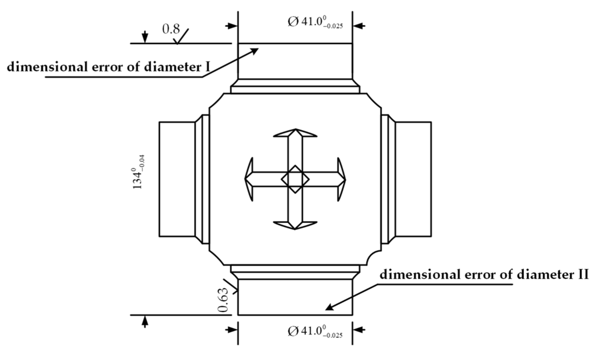
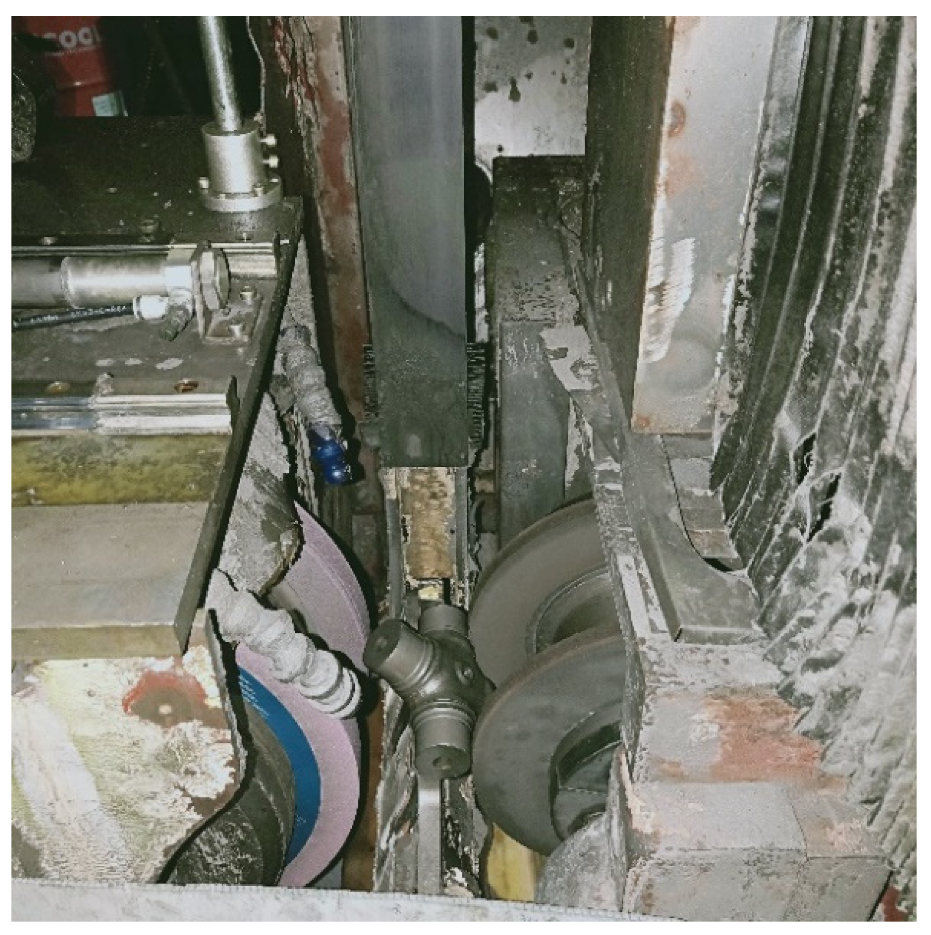
The chosen case is from a centerless grinding process which produces a heavy cross axis; the product drawing is shown in Figure 6. In addition, the grinding machine is shown in Figure 7.

It can be observed from Figure 6 that the dimension tolerance of the products is [−0.025, 0]. In addition, according to Figure 6, two diagonal axes are ground at the same time in the grinding process, so that two-dimensional errors (dimensional error of diameter I and dimensional error of diameter II) should be predicted together.

Furthermore, from previous experiments and arguments, the grinding force has a strong influence on the elastic deformation of the product during grinding, hence it is the key influencing factor for dimensional errors. Since grinding force is difficult to be detected and grinding power has a high correlation with grinding force, thus the grinding power is regarded as the main process feature to be studied. Moreover, considering that the fine grinding process and the spark out process have different effects on the final dimension of the product, therefore, after the experimental verification, the grinding power of the above process and its derived variables are selected as important input variables of the proposed algorithm. In addition, in view of the inconsistency of the workpiece, in this case, the 1–20th points of grinding power and other relevant derived variables (peak value of grinding power, etc.) are also selected as input variables.

Finally, the input variables of the proposed algorithm are shown as follows:

• The grinding power for the fine grinding process and the variables derived from it (average value, area of the power curve, slope, and variance), as recorded in

  Table 1. The grinding power of fine grinding process and its derived variables.

  Feature Parameter	Max	Min	Mean
  average value	6091.2	4151.9	4694.5
  area of power curve	97,482.5	69,439.5	75,425.7
  slope	1.5	−85.1	−17.7
  variance	540.1	22.2	121.1

  .
• The grinding power of spark out process and its derived variables (average value, area of power curve, slope, variance, peak value, mode value, median value, skewness, kurtosis, minimum value, end value, the ratio between the end power of spark out process and average power of fine grinding process as well as the ratio between end power of spark out process and peak of grinding power), as shown in

  Table 2. The grinding power of spark out process and its derived variables.

  Feature Parameter	Max	Min	Mean
  average value	3747.2	1912.7	2817.4
  area of power curve	108,518.5	55,368.5	81,432.0
  slope	−55.7	−120.0	−84.8
  variance	1188.8	509.9	853.8
  peak value	5709.0	3006.0	4434.9
  mode value	5295.0	1123.0	2701.9
  median value	3616.0	1877.5	2590.7
  skewness	1.0	−0.1	0.5
  kurtosis	2.9	1.3	2.0
  minimum value	2232.0	1015.0	1746.1
  end value	2297.0	1061.7	1793.4
  the ratio between the end power of spark out process and average power of fine grinding process	0.46	0.24	0.38
  the ratio between end power of spark out process and peak of grinding power	0.45	0.21	0.36

  .
• Other relevant derived variables of grinding power (peak value, the sum value of 1–20th points, the peak of first twenty points, the variance of first twenty points, the sum value of 40–128th points), as recorded in

  Table 3. Other relevant derived variables of grinding power.

  Feature Parameter	Max	Min	Mean
  peak value	6696.0	4608.0	4975.1
  sum of first twenty points	54,432.0	20,082.0	32,668.5
  peak of first twenty points	3534.0	1054.0	1909.1
  variance of first twenty points	716.6	7.9	192.2
  sum of values from 40th to 128th points	457,541.0	280,200.0	348,018.6

  .

Moreover, the raw datasets are randomly separated into 60% for the training set, 20% for the validation set, and 20% testing set, in which the training set and validation set are used in the training process of the bagging–GA–ELM model, the training set is used to determine the output weights of ELM model and the validation set is used to evaluate the fitness value of each chromosome in the optimization process of GA. Then a testing set will be used to evaluate the performance of the bagging–GA–ELM model.

3.1.2. Experiment Setup and Evaluation Indicator

The analysis of raw data acquired from the grinding process and all prediction experiments of dimensional error run in the Python 3.8 environment on a 3.20 GHz PC with processor i5-11320H and 16 GB RAM. Since the effect of randomness on the experiment results, all experiments in this research are run repeatedly three times and then averaged to obtain the final result.

In addition, the true positive ratio (TPR), false positive ratio (FPR), and corrected mean absolute percentage error (CMAPE) are used as evaluation indicators of prediction performance, the formulas of which are formed as Equations (15)–(17). Among evaluation indicators, TPR, as well as FPR, are used to evaluate the ability to identify quality problems. In addition, it is worth noticing that the traditional MAPE uses the observed value as the denominator. However, in this case, partially observed values of dimensional error are close to 0 mm, which will make the value of MAPE trend to infinity and make the performance of the prediction model unable to be evaluated accurately. Thus, CMAPE is designed in this case as the corrected value of MAPE, in which the value of tolerance (0.025 mm) will be used as the denominator.

According to Equation (17), if the predicted value deviated significantly from the observed value, the value of CMAPE will become large. On the contrary, when the difference between the predicted value and observed value is small, the value of CMAPE will be close to 0.

$$TPR=100\%\times TP/\left(TP+FN\right)$$

(15)

$$FPR=100\%\times FP/\left(FP+TN\right)$$

(16)

$$CMAPE=100\%\times {{\displaystyle \sum }}_{i=1}^n\left|y_{pre,i}-y_{obs,i}\right|/0.025$$

(17)

where $TP$ denotes the number of positive samples predicted as positive, $FN$ denotes the number of positive samples predicted as negative, $FP$ denotes the number of negative samples predicted as positive, $TN$ denotes the number of negative samples predicted as negative, $n$ denotes sample size, $y_{pre,i}$ and $y_{obs,i}$ represent the predicted value and the observed value of $i$th sample, respectively.

3.2. Parameters Optimization of Proposed Algorithm

It is considered that the different parameters of the proposed algorithm have an essential influence on the prediction performance of the dimensional error. Thus, the determination of main parameters (the main-relevant component number of PCA, the neurons number of hidden layer, and the number of the base learner) are discussed in detail in this section.

3.2.1. The Main Relevant Component Number of PCA

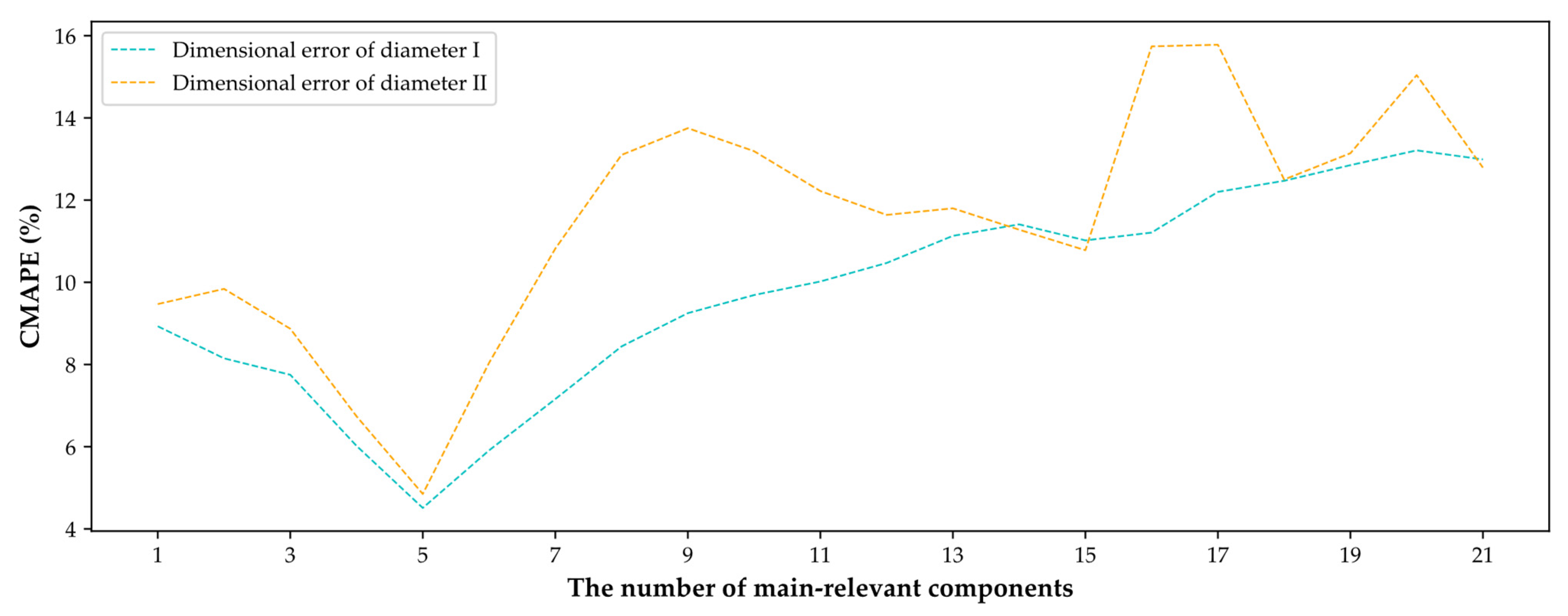
Adopting PCA in the pretreatment of data can extract main relevant components from feature parameters and remove negative noise, but it needs to be noted that excessive main relevant components can deteriorate the elimination effect of noise, while too few main relevant components lead to the loss of effective information. Therefore, the main relevant component number of PCA is analyzed and the performance ranking of different main relevant component numbers from 1 to 22 is shown in detail in Figure 8.

According to Figure 8, as the main relevant component number increases from 1 to 5, it is clear that the CMAPE on the testing set decreases significantly. Then, the optimal CMAPE is obtained when the main relevant component number is 5. With further increase of main relevant component number, the dimensional error of both diameter I and diameter II start to increase gradually, which means that the residual noise results in a reduction of generalization ability. Hence, the top five main relevant components are regarded as the final features extracted from data by PCA.

3.2.2. The Neurons Number of Hidden Layer and Parameters of GA

As a variant of ANN, the ability of ELM to deal with non-linear prediction problems mainly depends on the interconnection of neurons as well as the non-linear transformation of the hidden layer. Thus, the number of neurons in the hidden layer has high relation with the prediction accuracy of the proposed algorithm.

Obviously, the complex association between process parameters and dimensional error is difficult to be learned effectively by the prediction model with few hidden neurons. However, because of the limited information of raw data, too many hidden neurons will make the network parameters (input weights and thresholds) insufficiently trained, which usually results in overfitting problems.

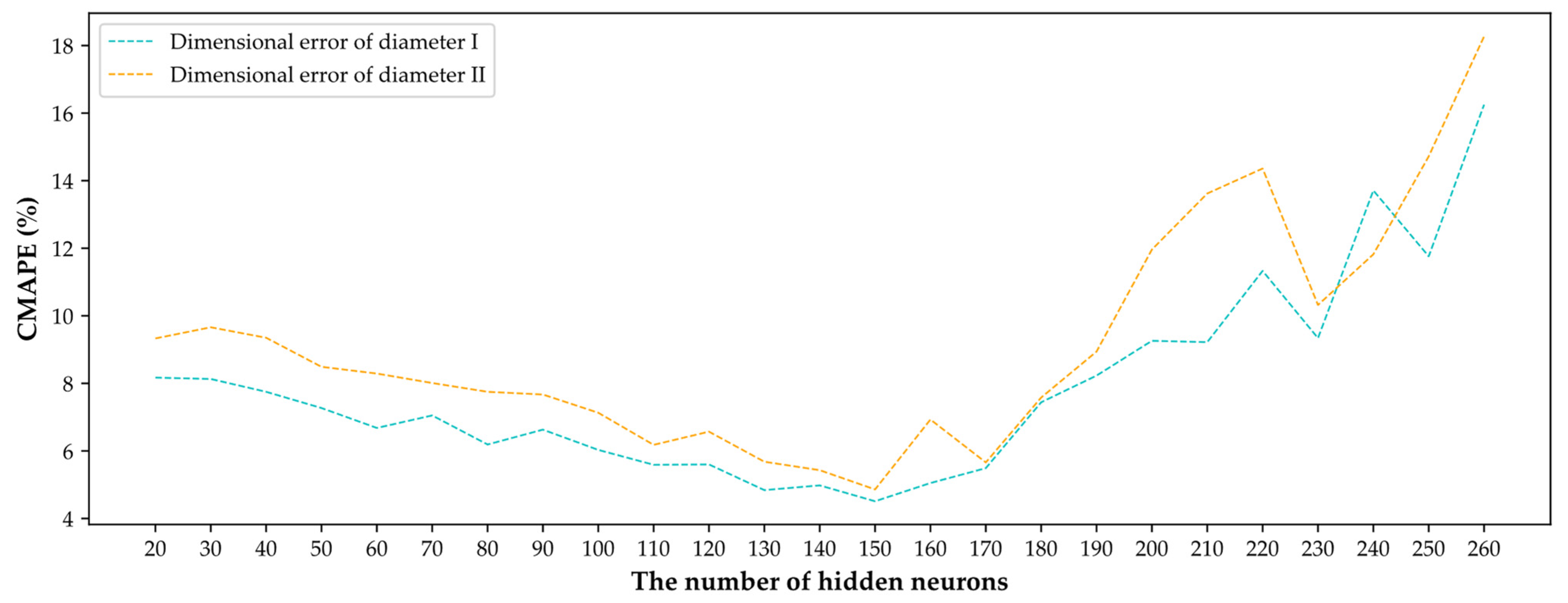
In order to obtain the optimal number of hidden neurons, the prediction performance of the proposed algorithm with different number of hidden neurons are compared by experiments. The result of experiments is shown in Figure 9.

As shown in Figure 9, with the increase of neurons from 20 to 150, the CMAPE of testing set will decline at first. On the contrary, when the number of hidden neurons is more than 150, the increasing neurons start to make the dimensional error fluctuate and increase, which indicates that the prediction model has a symptom of overfitting. As a result, the optimum of neuron number in the hidden layer is 150.

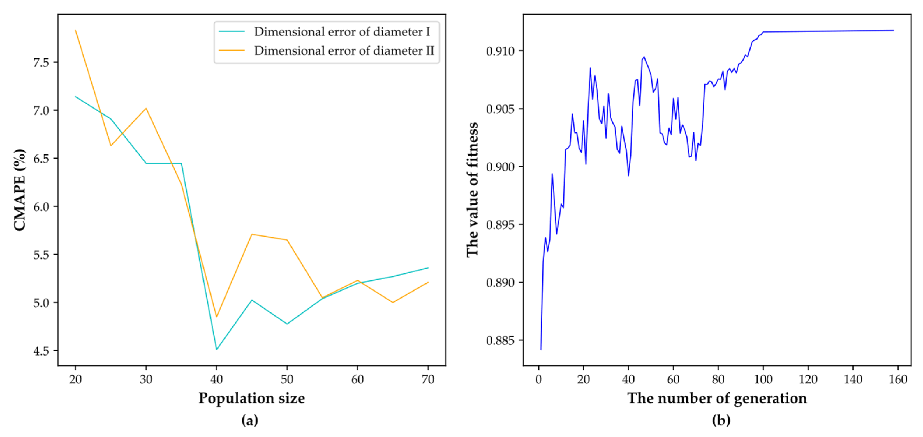
In addition, the genetic algorithm (GA) which has global optimization capability is combined with ELM to search the optimal network parameters, in which the population size and max generation of GA will be discussed in Figure 10.

According to Figure 10a, when the value of population size increases from 20 to 40, the CMAPE on the testing set decreases significantly; it is owing to that the increase in population size improves the diversity of chromosomes and the optimization effects of GA. However, with a further increase in population size, the curve tendency of CMAPE starts to slow down obviously. Thus, the optimal population size is set as 40. Further, in the view of Figure 10b, when the number of generations increases from 0 to 100, the fitness value increases significantly. However, when the number of generations is larger than 100, the further increase of generation number makes it difficult to obtain an effective improvement of fitness value. Thus, the optimal max generation is set as 100.

Furthermore, the genetic algorithm has been widely used to optimize parameters in the industrial field. Many experiments show that the crossover rate is usually larger than 0.9 to ensure the diversity of the population and the mutation rate is advised to be set lower than 0.05 [47]. Thus, the crossover rate and mutation rate in the evolution of chromosomes are set as 0.95 and 0.05, respectively.

Then, the comparisons between the ELM model and the ELM model optimized with GA (GA-ELM) are shown in

Table 4. The comparison between ELM model and GA–ELM model.

Model	CMAPE of Dimensional Error on Testing Set (%)
	Diameter I	Diameter II
ELM	7.74	10.68
GA–ELM	4.51	4.85

. Compared to the CMAPE of the ELM model, it can be observed that the CMAPE of the GA-ELM model achieves a significant reduction (the reduction rate of CMAPE in diameter I and diameter II are 41.73% and 54.58%, respectively), which shows the significant contribution of GA in accuracy improvement of dimensional error prediction.

3.2.3. The Number of Base Learners

In the proposed algorithm, the bagging algorithm is used to avoid the impact of noise in the real-time collected data, in which the GA–ELM model is used as the base learner. Then, various base learners are trained depending on different samples. After that, the outputs of these base learners are averaged to reduce the variance of the prediction results.

Since excessive base learners not only increase the time-consuming nature of the calculation process and the waste of computing resources but also have few contributions to the improvement of prediction performance, the optimal number of base learners should be determined carefully.

In this subsection, the influence of different base learner numbers on the prediction performance is studied, as shown in Figure 11.

It can be seen from Figure 11, that when the number of base learners increases from 1 to 25, the value of CMAPE declines significantly. However, when the number of base learners exceeds 25, the curve tendency of CMAPE starts to slow down obviously, which means that further increase of the base learner number makes it difficult to obtain effective accuracy improvement. Finally, the optimal number of base learners is set as 25.

Furthermore, the robustness of bagging–GA–ELM needs to be investigated because of the high complexity and strong interference in the industrial environments. In order to simulate the noise of real industrial environments, white Gaussian noise is added to the raw data. The intensity of white Gaussian noise is estimated by the signal-to-noise ratio (SNR), as formed in Equations (18) and (19).

To evaluate the robustness of the proposed algorithm, the prediction accuracy of the bagging–GA–ELM model and GA–ELM model are analyzed under various white Gaussian noise (SNR ranging from 1 dB to 10 dB); results are shown in Figure 12.

$$SNR=10lo{g}_{10}\left(P_r/P_n\right)$$

(18)

$$P_r={{\displaystyle \sum }}_{i=1}^n{A}_{r,i}/n, P_n={{\displaystyle \sum }}_{i=1}^n{A}_{noise,i}/n$$

(19)

where $n$ denotes sample size, $P_r$ and $P_n$ denote the signal power of raw data and noise, respectively, $A_{r,i}$ and $A_{noise,i}$ represent the i-th amplitude value of raw data and noise, respectively.

It is clear from Figure 12, with the reduction of SNR, the interference of noise becomes obvious gradually and makes the CMAPE of both models start to increase. However, in comparison with the GA–ELM model, the CMAPE of bagging–GA–ELM is much lower than that of the GA–ELM model, which obviously shows the contribution of the bagging algorithm in the improvement of anti-interference ability.

3.2.4. The Structure of Proposed Algorithm

Based on the above discussions, the structure of the proposed algorithm has been determined as follows:

The raw data acquired from the grinding process is a matrix of N × 22, which means that there are N samples and each sample has 22 feature parameters. Then, the matrix will be normalized at first and the PCA is used to transform 22 feature parameters into five main relevant components to remove the redundant information as well as noise. Next step, the five main relevant components will be regarded as the inputs (N × 5) of the ELM model.

The ELM model has three layers (input layer, hidden layer, and output layer), in which the input layer has 5 neurons, the hidden layer has 150 neurons and the output layer has 2 neurons. Thus, the output of the proposed algorithm is a matrix of N × 2, which means that there are N samples and each sample has two prediction results (diameter I and diameter II).

3.3. The Dimensional Error Prediction in Grinding Process

In this section, the performance of bagging–GA–ELM is further discussed. Firstly, the bagging–GA–ELM will be compared with other prediction models (KSVM and ANN) to analyze its accuracy and calculation speed. Next, the proposed algorithm is applied to analyze the raw data acquired from the grinding process and shows the results of dimensional error prediction.

3.3.1. Comparisons of Prediction Models

Since KSVM and ANN are widely used in the field of industrial analysis, which are regarded to have characteristics of high accuracy and strong universality by practice. So as to evaluate the dimensional error prediction performance of the proposed algorithm in the grinding process, the above models are used to compare to the bagging–GA–ELM model, and the parameters of these models are recorded in

Table 5. The parameters of different prediction models.

Model	Parameters	Value
KSVM	Kernel	Gaussian
	Penalty coefficient	1
ANN	Hidden layer	5
	Hidden neurons	25, 50, 150, 50, 25
Bagging–GA–ELM	Hidden neurons	150
	Max generation	100
	Number of base learners	25

. In addition, the comparisons among different prediction models are shown in

Table 6. The comparison among different prediction models.

Model	CMAPE of Dimensional Error on Testing Set (%)
	Diameter I	Diameter II
KSVM	12.03	11.54
ANN	5.78	6.33
Bagging–GA–ELM	3.20	3.01

.

According to Table 6, it is clear that the CMAPE of KSVM is higher than other models, which is related to the complexity of dimensional error prediction as well as the ability to deal with the non-linear problem. Moreover, it can be further found that the bagging–GA–ELM model achieves the optimal performance in prediction (the CMAPE of dimensional errors on the testing set are 3.20% for diameter I and 3.01% for diameter II, respectively).

3.3.2. Prediction Results Based on Proposed Algorithm

Based on the proposed algorithm, the dimensional error of products will be predicted during the grinding process. Once the predicted dimensional error exceeds the dimension tolerance, the process will be stopped and the alarm will be generated and relative information will be sent to operators to prevent a further quality problem. Thus, although the accuracy and robustness of the proposed algorithm have been verified in the above discussions, the ability of the proposed algorithm to identify the quality problem is further to be evaluated.

Considering that the difference between the number of products with a quality problem (namely positive samples) and the number of products without a quality problem (namely negative samples) is usually significant, it is necessary to investigate the identification rate of positive samples and negative samples, respectively. Therefore, the true positive ratio (TPR) and false positive ratio (FPR) are used as evaluation indicators of identification performance, in which TPR is used to evaluate the rate of positive samples predicted as positive, and the larger value of TPR denotes the higher identification performance on the positive samples. In addition, FPR is used to evaluate the rate of negative samples predicted as positive, so that the smaller value of FPR denotes the higher identification performance on the negative samples.

Therefore, based on the TPR and FPR, the identification performance of the proposed algorithm is evaluated and compared to other models, as shown in

Table 7. The identification performance of quality problems under different background noise.

Model	Diameter I		Diameter II
	TPR (%)	FPR (%)	TPR (%)	FPR (%)
KSVM	89.61	13.56	86.83	15.14
ANN	94.78	4.89	91.16	6.21
Bagging-GA-ELM	99.48	0.36	99.32	0.98

.

According to Table 7, it can be observed that bagging–GA–ELM achieves the best identification performance in both diameter I and diameter II. The values of TPR are higher than 99% and the values of FPR are lower than 1%, which means that the success rate of the proposed algorithm achieves more than 99% in the identification of the real-time collected data. Therefore, the proposed algorithm can be used to identify the quality problem accurately, which meets the requirement of the production line.

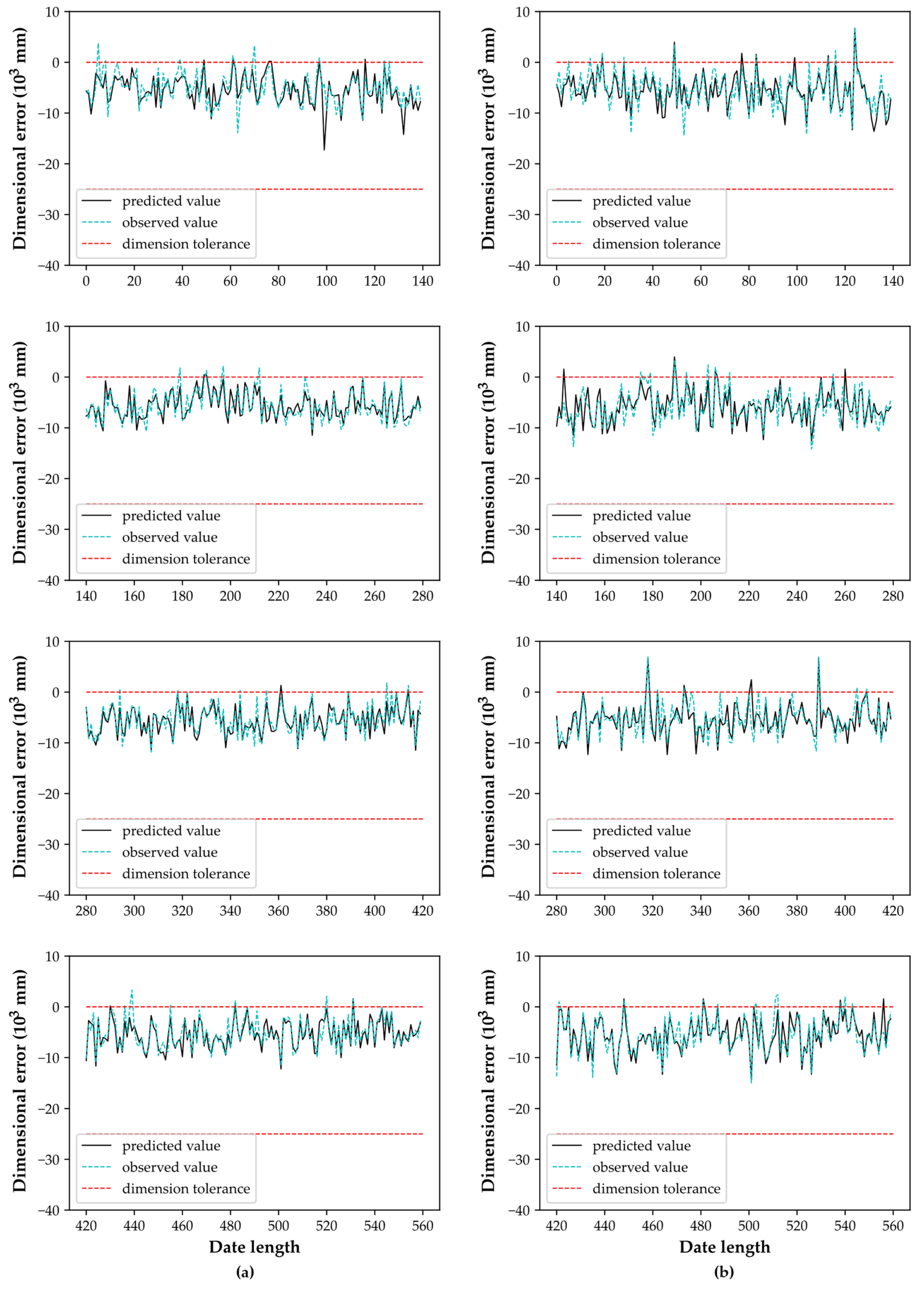
Finally, based on the proposed algorithm, the prediction results of data acquired from the real-time grinding process are shown in

Table 8. The comparison between the actual dimension error (ADE) and the predicted dimension error (PDE).

Data	Mean	Std
	10−3 mm	10−3 mm
ADE of diameter I	−5.32	3.03
PDE of diameter I	−5.35	2.37
The absolute difference between ADE and PDE in diameter I	0.79	1.27
ADE of diameter II	−5.46	3.48
PDE of diameter II	−5.47	2.89
The absolute difference between ADE and PDE in diameter II	0.75	1.49

and Figure 13.

4. Conclusions and Future Work

In this paper, an approach based on bagging–GA–ELM is proposed to predict the final part dimensional error during the grinding process with high accuracy and robustness. In particular, firstly, the raw data are pre-processed to eliminate the dimensionality of the data while avoiding negative noise. Then the bagging–GA–ELM, which combines the advantage of ELM with short training time, GA with global optimization ability, and bagging with good anti-interference ability, is used to predict the dimensional error of parts. The experimental performance shows that the proposed algorithm achieves the best dimensional error prediction performance compared with the KSVM model and ANN model. In addition, the proposed algorithm has achieved good quality problem identification performance (success rate of more than 99%), which can satisfy customers’ requirements. Additionally, the application of the algorithm in the bearing company helps to save additional investment in equipment.

In the future, we intend to continue our research in the parameters of the grinding process to improve the prediction success rate. By doing this, the grinding process can be better controlled. In addition, we will also study the proposed algorithm in other products.