Abstract
Time-series forecasting is the core of the prognostics and health management (PHM) of turbomachinery. However, missing data often occurs due to several reasons, such as the failure of sensors. These partially missing and irregular data greatly affect the quality of time-series modeling and prediction as most time-series models assume that the data are sampled uniformly over time. Meanwhile, the training process of models requires a large number of samples and time. Due to various reasons, it is difficult to obtain a significant amount of monitoring data, and the PHM of turbomachinery has high timeliness and accuracy requirements. To fix these problems, we propose a multi-task Gaussian process (MTGP)-based data imputation method that leverages knowledge transfer across multiple sensors and even equipment. Thereafter, we adopt long short-term memory (LSTM) neural networks to build time-series forecasting models based on the imputed data. In addition, the model integrates the methods of denoising and dimensionality reduction. The superiority of this integrated time-series forecasting framework, termed MT-LSTM, has been verified in various data imputation scenarios of a synthetic dataset and a real turbomachinery case.
1. Introduction
Turbomachinery, such as steam turbines, turbocompressors, and gas turbines, is the key equipment type in the electric power, metallurgical, petrochemical, and aviation industries supporting the national economic lifeline. With the development of technology, turbomachinery is heading toward high levels of speed, integration, precision, and intelligence. High availability and reliability standards must be satisfied [1,2]. However, due to their complex structures, special operating environments, and long service time, the failure rate of turbine units is high, which creates serious damage. Therefore, the prognostics and health management (PHM) of turbomachinery, which involves health monitoring, feature extraction, fault diagnosis, and fault forecasting, has emerged as a crucial issue that must be resolved [3,4].
The main research object of PHM is multivariate time-series data. The acquired original data are distinguished by high accuracy, wide coverage, variable patterns, different correlations, and rapid evolution due to the widespread use of inexpensive sensors and the growth of the Internet of Things. Tools for robust multivariate time-series modeling and analysis are urgently needed. The two main kinds of existing approaches are data-driven methodology and physics-model-based methodologies. The physics-model-based approaches must provide a thorough mathematical model to represent the system’s physical properties and fault mechanisms [5,6], whereas, building a physical model of complicated mechanical systems is challenging, and the approaches rely on domain knowledge, which limits the viability and adaptability of these approaches. The challenge of fault diagnosis in complicated mechanical systems is made easier by data-driven approaches. Hence, data-driven methods have gained widespread attention. Data-driven models have experienced two stages [7]. The first is traditional intelligent models based on machine learning (ML). This paradigm extracts statistical features of signals in the time domain, frequency domain, or time–frequency domain and feeds them into ML models such as support vector machines (SVM) [8], k-nearest algorithm [9], or naive Bayes [10] to identify the status of equipment. In traditional ML methods, many efforts have aimed at the manual design of feature extraction algorithms as traditional models cannot extract representative features from raw signals. Such feature-designing processes require abundant professional knowledge and experience, which necessitate a significant amount of human labor, which limits the application of these kinds of methods. The second is modern intelligent models based on deep learning (DL). In contrast, this end-to-end paradigm directly feeds the raw signals (time domain) or pre-processed signals (frequency domain and time–frequency domain) into the deep neural network model to learn the mappings between data and status [11].
Deep learning (DL) is the most popular embranchment of machine learning and has created significant progress in a wide range of areas [12]. Usually, DL-based methods construct a multi-layer structure to extract deeper and more essential features. Recently, various DL-based methods, for example, restricted Boltzmann machines (RBM) [13,14], convolutional neural networks (CNN) [15,16], recurrent neural networks (RNN) [17], auto-encoders (AE) [18], long short-term memory (LSTM) networks [19], or their variants [20,21] have been widely investigated. They can adaptively obtain effective features from time-domain, frequency-domain, and time–frequency-domain data. Then, the system’s operating state can be identified by inputting the features into the regressor or the classifier. However, the training of DL models requires many samples, which is difficult to achieve in practice due to their scarcity. Moreover, the training process requires a lot of time as each layer needs a huge number of training epochs [22,23].
To resolve the first drawback, Lim et al. [24] proposed an expedient assessment framework of LED reliability. Multi-output Gaussian process regression (MOGPR) was performed on sparse reference data to establish an accepfigure threshold for the degradation signature. The framework achieved a reduction in the validation time from 6000 h to 100 h. Jia et al. [25] presented a method named deep normalized convolutional neural network (DNCNN) with normalized layers and a weight normalization strategy. This approach effectively increases the fault diagnosis accuracy with a limited number of fault samples. Ensemble deep auto-encoders (EDAEs), a framework that includes several auto-encoders with various properties, was proposed by Shao et al. [26]. The accuracy of this approach can reach 93.5% when there are 12 health statuses of bearings and 100 fault samples. Based on the generative adversarial network (GAN), Mao et al. [27] proposed a fault diagnosis approach. The fault diagnosis model’s generalization ability was improved by generating synthetic samples for the minority fault class. However, deep neural networks form the foundation for the above methods. We know this requires significant training time and epochs, which impedes the model’s ability to update quickly.
To resolve the second drawback, Guo et al. [23] proposed a CNN–LSTM deep learning model-based method for fault diagnosis on the hydraulic system of the blanket transfer device Mover in the Chinese Fusion Engineering Test Reactor (CFETR). In the fault diagnosis experiment, the model had the highest accuracy of 98.56% on the test set and good efficiency in computation time compared to the other three models. Wang et al. [22] obtained a stable distribution of activation values in training by putting batch normalization (BN) in each layer of SAEs. This method can reduce the training time and epochs. Qin et al. [28] proposed a new activation function, Isigmoid, which combines the traditional Sigmoid with ReLU. The results showed that the approach found a solution to the vanishing gradient in the backpropagation process of the deep network and has advantages in convergence. Zhuang et al. [29] presented a new method called multi-scale deep convolutional neural network (MS-DCNN). This intelligent method extracts characteristics of various sizes in parallel using convolution kernels of different sizes, which has a better learning effect, stronger robustness, and reduced training time. Unfortunately, none of the approaches mentioned above can be used for few-shot learning or missing data.
To overcome the above disadvantages, we design a multi-task time-series data analysis model for the health management of turbomachinery. To account for the scarce-data scenario in the PHM of turbomachinery, we performed data imputation of the target task by leveraging knowledge from auxiliary data (tasks) through the modeling of a multi-task Gaussian process (MTGP), which is a non-parametric multi-task model. Thereafter, we employed long-short term memory (LSTM) to build the sequence model of the target data upon the imputed time-series data to perform a prediction in the future. Meanwhile, we integrated denoising and dimensionality reduction techniques. In comparison to solely modeling the scarce sequence data of the target task, the proposed multi-task LSTM (MT-LSTM) provides more accurate and efficient modeling and predictions, which thus benefits downstream fault diagnosis, remaining useful life estimation, etc.
The remainder of this paper is structured as follows. In Section 2, we expound on the theory and ingredients of the proposed multi-task time-series data analysis model. Section 3 conducts empirical research to verify the superiority of the proposed model. Finally, Section 4 summarizes the conclusions.
2. Methods
For the time-series forecasting of the performance of turbomachinery, missing data is commonly encountered due to the failure of sensors or human error, and it greatly affects the quality of time-series modeling and prediction. Therefore, it is important to fill in the missed time-series data before forecasting. The turbomachinery operation datasets, meanwhile, often have the following characteristics: time series with noise, non-significant periodicity, and high and correlated dimensions (multi-task). Hence, we need to integrate multiple methods, including data denoising, dimensionality reduction, normalization, imputation, and prediction. The flowchart in Figure 1 presents the process for time-series forecasting using datasets collected from turbomachinery. Suppose that we collected scarce time-series data (target task) regarding the interested performance indicator of turbomachinery, and some related and sufficient time-series datasets (auxiliary tasks) collected from other performance indicators are available. The proposed MT-LSTM first performs data denoising using discrete wavelet packet transform (DWPT), followed by a reduction in dimensionality via probabilistic principal component analysis (PPCA). Thereafter, the MT-LSTM conducts the data imputation of the target task through MTGP. Finally, the LSTM model is built upon the imputed data to predict of the target task in the future. The following sections elaborate on the key ingredients in the proposed MT-LSTM model.
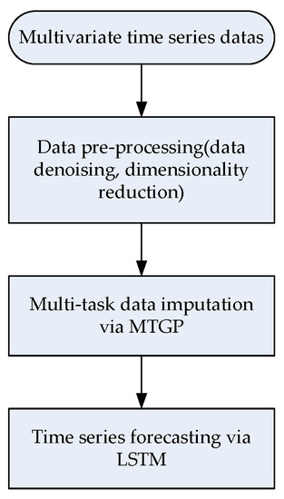
Figure 1.
Flowchart of the proposed MT-LSTM method.
2.1. Data Denoising
In the complex working environment of turbomachinery, sensor time-series data usually comprise a wide range of defects, for example, noise, error, and incoherence. Hence, it is necessary to remove the noise or uncertainty characteristics of data before modeling. In past decades, scholars have proposed many methods to remove noise from sensor data. However, few studies have evaluated multiple defects simultaneously. In this paper, we propose Bayesian wavelet denoising and use multiscale wavelet analysis to analyze the contexts in the signal.
Specifically, we adopt discrete wavelet packet transform (DWPT) to denoise and multiscale analyze the original time series. In DWPT, a given one-dimensional time-series signal, , with historical data points, is simultaneously decomposed into a sequence of scaling coefficients, , and wavelet coefficients, . Then, we can use the inverse wavelet transform and the DWPT coefficients to reconstruct the time series as follows:
where is the reconstructed time series; and are the time and frequency indices, respectively; is the scaling function; is the wavelet function; and the double summation means that the wavelet subspace and scaling subspace are simultaneously decomposed into second-level subspaces, which reveal the time and frequency resolution of the signal.
For the benefit of universality, we set to the -th decomposed coefficients at the -th level ( = , …, − 1; = 0, 1, …, − 1). According to the Bayesian rule, the posterior distribution of the cleaned coefficients, , can be expressed as
where the symbol ~ represents a distribution; denotes a normal distribution, where is the mean and is the variance; denotes the decomposed coefficients distribution, ; is a binary random variable with independent Bernoulli distribution , i.e., P( = 1) = 1 − P( = 0) = , which decides whether are zero ( = 0) or nonzero ( = 1); and the variance denotes the magnitude of at the -th decomposition level. For all the coefficients in the -th level, and may be assigned the same values; is the standard deviation, which is estimated from the wavelet coefficients of the -th level DWPT decomposition by dividing the median of the wavelet coefficients by a factor.
Then, the Bayesian hypothesis test is applied to threshold the decomposed coefficients by determining whether to accept the null hypothesis, : = 0. The thresholding rule is defined as follows:
where is the posterior odds ratio of = 0 versus = 1. I(.) denotes an indicator function. When < 1, I(.) is equal to unity. Thus, is rejected and estimates the coefficient . If not, I(.) is equal to zero, and is removed. The cleaned time series based on Equation (1) is then reconstructed by using the acquired coefficients from Equation (3).
In summary, we can decompose the time-series data into various levels of wavelet coefficients by the DWPT analysis. Then, a Bayesian hypothesis test is carried out for each level of wavelet coefficients to eliminate possible defects. To avoid over-denoising, the ratio of posterior odds Bayesian method offers a simple way to determine whether the decomposed coefficients have any defects. Meanwhile, the DWTP method provides more coefficients denoting additional subtle details of the time-series signal, thus avoiding under-denoising.
2.2. Dimensionality Reduction
In the analysis of multi-variable time-series data of turbomachinery, due to the correlation between variables and the inherent uncertainty of data, too many variable dimensions increase the calculation assumption and the analysis complexity. After cleaning the multivariate time-series data, the PPCA method is mainly used to (1) reduce data dimensionality, (2) decouple the multivariate correlation, and (3) filter data uncertainty. The method plays an important role in improving the accuracy of subsequent data analysis and reducing the calculation time.
Let represent a -dimensional real number and let represent the × data matrix: there are variables, and each variable contains cleaned time-series data points, . Let represent the × data matrix and represent unobservable latent variables (factors), each contains corresponding positions in the latent space. All are usually defined as independently distributed Gaussian variables obeying zero mean and unit variance, i.e., . The latent variable model combines the measurable variable in the relevant data matrix with the corresponding uncorrelated latent variable matrix . Then, the form of the Gaussian distribution is
where is the isotropic noise covariance, the × weight matrix represents the relation between and , and mean values that are acquired from form the parameter vector , i.e., . In the lower dimensional latent space, the unadjusted data can be expressed as
where , , and are the maximum likelihood of and . Equation (5) has the mean of . The -dimensional principal components (PC) matrix is used in the following data-driven modeling.
2.3. MTGP Model
In the data analysis of turbomachinery, the lack of data is often caused by the damage of sensor equipment, the insufficient maintenance of equipment, the power failure of equipment, the aging fault of equipment hardware and software, the communication interruption of equipment, and new equipment recently put into operation. Data imputation and augmentation are crucial to the performance of the deep learning model for time-series data, which can effectively improve the size and quality of the training data. We explore a method for time-series data imputation using the multi-task GP model.
We assume a given dataset T = , , is specified as the index set, such as the observed time, and is the corresponding value of the observed training data. The purpose is to learn a regression model: , where is a latent function and is a noise term. Given the test points , we can predict the uncharted test observations .
Gaussian processes (GP) are useful for time-series modeling [30] because they can accommodate irregular and uncertain observations, and provide probabilistic predictions. Gaussian process models suppose that can be expressed as a probability distribution of the following functions:
where is the mean function and is a covariance function describing the coupling between the inputs. The prior knowledge of the function behavior, which we want to model, can be encoded by modifying the covariance function. In the covariance of the vector , the size of the covariance matrix is , and the covariance function provides the element . The covariance function usually satisfies Mercer’s theorem; that is, must be symmetric and positive semidefinite. The affine transformation of the basic covariance function can be used to construct the complex covariance function.
For a given set T, we can obtain the predictions at the test indices through calculating the conditional distribution , where is a Gaussian distribution:
where is the mean and is the variance. Without the loss of generality, it is usually assumed that the mean function is zero. Thus, and can be expressed as
Furthermore, we assume that are the training indices, and are the observations for tasks, where task has training points. In an actual situation, we may encounter task-specific with training indices where the number is far lower than the other tasks. This is a challenge for the problem.
The problem of modeling tasks simultaneously (e.g., multiple time-series) drives the extension of the MTGP model, where all models have the same index set . Training an STGP (single-task GP) model for each task separately is a straightforward method, as shown in Figure 2a. For the modeling of tasks via MTGP, to reveal the affiliation of index and observation to task , we have to add a label to the model as an additional input with , as illustrated in Figure 2b.
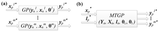
Figure 2.
Box diagram of (a) multiple STGPs and (b) MTGP for multi-task modeling.
In MTGP, two independent covariance functions, and , can be assumed as
where denotes the correlation between tasks and only depends on the labels and denotes the temporal covariance functions within a task and only depends on the indices . Let for ; the covariance matrix can be expressed as
where ; ⊗ is the Kronecker product; and are vectors, including hyperparameters for and ; has a size of ; and has a size of . Thus, the matrix, has a size of . We named as the correlation matrix. In practice, to adapt the model to the usage of task-specific training data, we can relax the assumption for .
This model has some useful features: we may have task-specific training indices (i.e., training data may be observed at task-specific times); when fitting the covariance function in (11), the correlation within the tasks can be learned automatically; the tasks have analogous temporal characteristics and hyperparameters in the framework assumption.
In summary, as MTGP is not a parametric approach, the number of parameters can grow as more observation data are collected. The advantage of the MTGP model over other comparable related methods, such as support vector regression (SVR), is that it may easily express prior knowledge of function behavior (e.g., periodicity or smoothness). Given multiple time series, the goal is to increase the overall modeling accuracy by employing a single MTGP model rather than several STGPs. MTGPs have been used in financial time series [31], environmental sensor networks [32], and the classification of ECG signals [33]. It is important to note that MTGPs can include nonuniformly sampled time series in a single model without further downsampling or interpolation. In addition, it is easy to include prior knowledge between time series, such as time shifts or assumptions about similar temporal. Thus, the method has many applications, such as prediction, correlation analysis, the estimation of time shifts between signals, and the compensation of missing data.
2.4. LSTM Model
It is very important to predict the operation trend for turbomachinery reliability. Recurrent neural networks (RNN) can predict trends quickly and accurately. However, the traditional RNN has the problem of gradient disappearance or explosion and cannot solve long-term dependence, which affects its practical application [34]. To solve this problem, we established a prediction model based on LSTM (long short-term memory). The LSTM is an improvement on RNN [35], which is composed of multiple connected recurrent units recursively. Three gate structures, i.e., forgetting gate, input gate, and output gate, constitute the recurrent unit of LSTM [23]. The advantages of LSTM are mainly embodied in the following aspects: (1) the three gating structures of LSTM can learn long-term memory information and provide a solution to long-term dependence; and (2) the sigmoid function and tank function are combined to form the activation function in LSTM, which keeps the gradient almost unchanged during the derivation of backpropagation, avoiding the disappearance or explosion of the gradient, and greatly accelerating the convergence speed of the model.
The LSTM neural network has a variety of input forms. Here, we consider the univariate time-series data. We suppose that there are discrete time points with a uniform distribution, and is a multi-dimensional time variable at each observed time point. These random variables serve as the input of the LSTM neural network.
According to Figure 3, at time , LSTM receives three inputs: the network’s input in the present, the previous time output , and the previous time cell state . At the same time, LSTM has two outputs: output and cell state . We can notice that , , and are all vectors. LSTM has three gate-like structures that filter through the information [36,37].
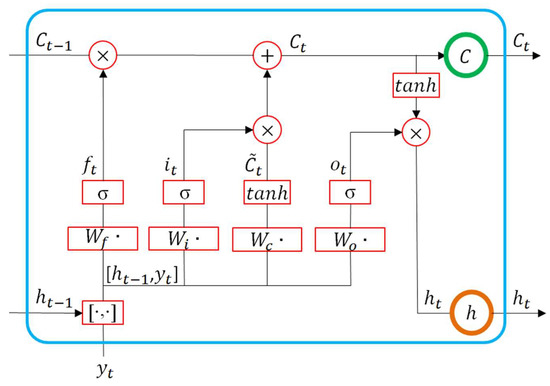
Figure 3.
LSTM neural network and its unrolled form.
The forgetting gate controls how much information of the previous time cell state is passed to at the present time:
where is the sigmoid activation function, is the weight matrix of the forgetting gate, and is the bias.
The input gate controls how much information of input is passed to at the present time (i.e., it is used to update the cell state):
where is the input gate, is the weight matrix of the input gate, and is the bias. is the input cell state, is the weight matrix of the cell state, and is the bias of the cell state.
The output gate determines how much information of is passed to the present output :
where is the output gate, is the weight matrix of the output gate, and is the bias. The final output of the LSTM is determined by the output gate and the cell state.
3. Experiments and Results
In the following sections, we first illustrate the performance of the proposed MT-LSTM on an optical marker (OM) dataset. Thereafter, the superiority of MT-LSTM is further verified on a real turbine operation dataset.
3.1. OM Dataset
We first investigated whether the proposed MT-LSTM could augment scarce time-series data among multiple tasks and improve prediction accuracy. We used multivariate biomedical data from the literature [38]. These data consisted of three optical markers (OM) time series that were located at the midline of the body: the thorax (OM1), the lower breastbone (OM2), and near the navel (OM3). The three-dimensional positions of all sensors were simplified as their first principal component. In addition, the fourth task corresponded to a respiration belt (RB) placed around the torso near OM2. The monitoring time and sampling frequency (2.6 Hz) were the same for all tasks. Each task included 200 data points, as shown in Figure 4. We investigated two situations—a normal situation and an extreme situation—to prove the method’s validity. The normal situation included a few missing data (named S1) and different sampling frequencies (S2). We named the extreme situation S3. It is important to note that since the OM dataset was clean and low-dimensional, we did not conduct data pre-processing such as data denoising and dimensionality reduction (Figure 1).
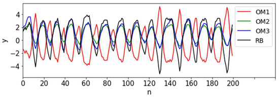
Figure 4.
Time-series signals of the 4 tasks from the OM dataset. x-axis: n is the number of data points.
In this paper, we used some indicators to evaluate prediction accuracy. The predicted test observations are denoted as . We used the mean absolute error (MAE), root mean square error (RMSE), and mean absolute percentage error (MAPE), defined as
Lower MAE, RMSE, and MAPE indicate higher prediction accuracy.
3.1.1. Multi-Task Data Imputation
- (1)
- S1—Few data missing
For the S1 case, we assumed that a few data were missing for each of the four tasks (OM1-3, RB). Specifically, each task picked the first 150 data points and had 30 data points removed at different time points. Figure 5 and Table 1 show the imputation and error results of each task using MTGP and STGP. Obviously, the MTGP model fit well with the original data of each task by transferring knowledge across tasks. The results were very accurate, and the related MAE and RMSE were close to 0. In contrast, for the results of STGP, it was impossible to observe the trend of the tasks, and the corresponding MAPE was much larger than that of MTGP.
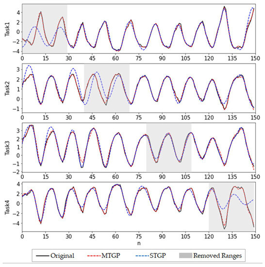
Figure 5.
Imputation results of MTGP and STGP for S1.

Table 1.
Error results of MTGP and STGP for S1.
- (2)
- S2—Different Sampling Frequencies
For the S2 case, we assumed that the sampling frequency of the tasks was different. In practice, the different sampling frequencies of various sensors led to different data volumes of signals, which introduced challenges to the subsequent modeling. We set the sampling frequency of Task 3 to be half that of the other tasks, i.e., Task 3 had only 75 data points. Tasks 1–2 and Task 4 had 30 data points removed (same as S1). As shown in Figure 6 and Table 2, the MTGP was found to effectively model these tasks with different sampling frequencies and have accurate predictions.
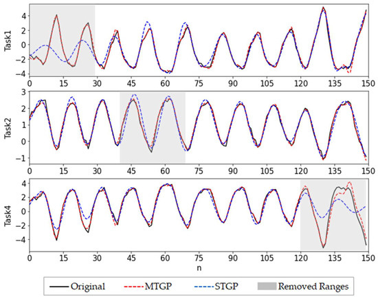
Figure 6.
Imputation results of MTGP and STGP for S2.
Table 2.
Error results of MTGP and STGP for S2.
3.1.2. Time-Series Forecasting via Multi-Task Data Imputation
For the S3 case, we considered an extreme case—some tasks had very scarce data at finite early time points. For Task 1, we kept the first 13 points and removed the remaining 137 data points (91.3% data missing), which eliminated the periodicity of the data itself. The other tasks were kept unchanged. We predicted that the few-shot scenario would undoubtedly introduce great challenges to data augmentation and prediction.
First, we performed data imputation for Task 1 with STGP. As shown in Figure 7, the predictions quickly failed. Next, we used the MTGP model and observed significantly improved predictions (Figure 7). This was also verified in Table 3, which showed that in comparison to STGP, the RMSE of MTGP decreased sharply from 2.128 to 0.648. Consequently, the prediction results of the MT-LSTM in Figure 8 and Table 4 were also more accurate predictions in comparison to the ST-LSTM based on STGP. Moreover, when the incomplete data (13 data points) were directly used for LSTM training, the predictions were extremely inaccurate (see Figure 8 and Table 4).
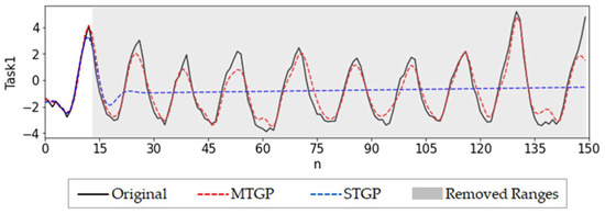
Figure 7.
Imputation results of MTGP and STGP for S3.
Table 3.
Error results of STGP and MTGP for S3.
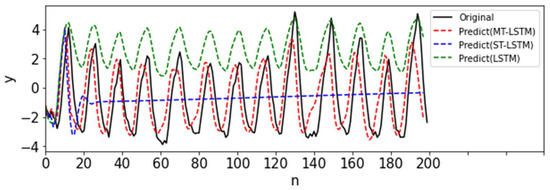
Figure 8.
Prediction results of MT-LSTM, ST-LSTM, and LSTM for S3.
Table 4.
Error results of MT-LSTM, ST-LSTM, and LSTM for S3.
Hence, the validity of the proposed MT-LSTM was preliminarily verified on the OM dataset.
3.2. Real-World Datasets
The performance of our method was verified on a set of actual turbine operating data. In a large centrifugal compressor manufacturing enterprise, more than 10 compressors suffered accidents during operation in several years, many of which were new units recently put into operation, resulting in huge losses. Meanwhile, some accidents were accompanied by sensor failures. To analyze these accidents, we studied one of the compressor units. After the new compressor was brought into service, the vibration condition and the amplitude were stable at about 20 μm, which was much lower than the alarm value. However, the vibration value rose and exceeded the alarm value after more than 10 days of operation. It is obvious that the scarcity of available data poses significant challenges to this research. The original time-series data were obtained from various sensors positioned on the centrifugal compressor, and the deployment of the sensors is shown in Figure 9. The collected data contained various operating parameters: for example, inlet and exhaust pressure, exhaust flow, bearing temperature, and axis vibration. The sensors measured the operating data every hour, and a total of 11 performance variables were collected in the same time period in this paper. Hence, there were 11 tasks, each with only 200 data points. Obviously, these data contain noise. Table 5 shows the details of the tasks.
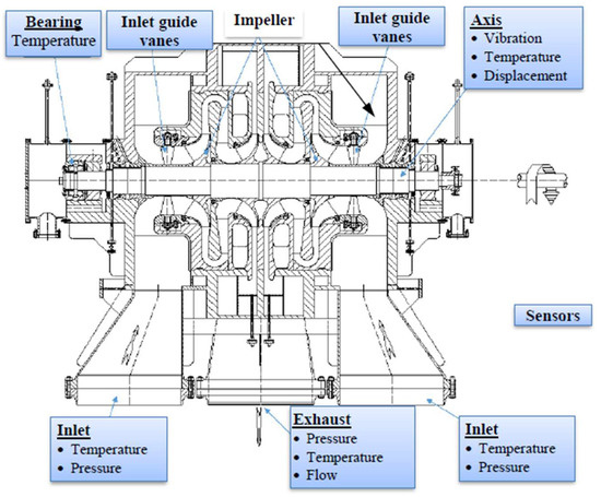
Figure 9.
Diagram of sensors used to acquire time-series data from a centrifugal compressor.
Table 5.
Details of tasks acquired from the centrifugal compressor.
If we consider an extreme case such as S3 in the OM dataset, some tasks had very scarce data collected at the early time points. Specifically, each task picked the first 150 data points. For Task 10, we kept the first 20 data points and removed the remaining 130 data points (86.7% data missing). The other tasks were unchanged.
3.2.1. Results without Data Pre-Processing
The MT-LSTM method we propose in this paper was applied to this dataset. First, we used the MTGP model directly without data pre-processing. The calculation procedure was the same as that for the S3 of the OM dataset. Figure 10 and Table 6 show the results. It was found that the imputation results of STGP failed quickly, and the prediction variance was high. As expected, the predictions of MTGP improved significantly over STGP. Consequently, the prediction of MT-LSTM achieved the best results (Figure 11 and Table 7).
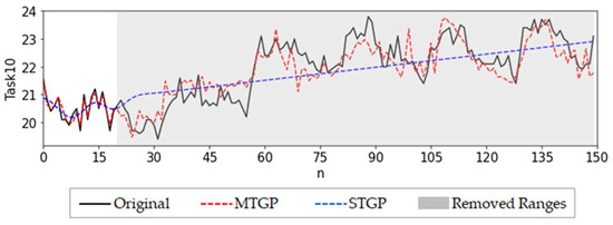
Figure 10.
Imputation results of MTGP and STGP for the extreme situation.
Table 6.
Error results of STGP and MTGP for the extreme situation.
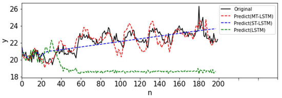
Figure 11.
Prediction results of MT-LSTM, ST-MTGP, and LSTM for the extreme situation.
Table 7.
Error results of MT-LSTM, ST-LSTM, and LSTM for the extreme situation.
3.2.2. Results with Data Pre-Processing
To investigate the impact of data pre-processing, we first normalized each task before MTGP modeling. The aim was to lessen the influence of various data value scales as normalization can compare multiple time-series variables at the same time. It prevents large-valued variables from overcontrolling small-valued variables, which improves accuracy. As shown in Figure 12 and Figure 13, Table 8 and Table 9, the MTGP and MT-LSTM results were improved compared to those without data pre-processing.
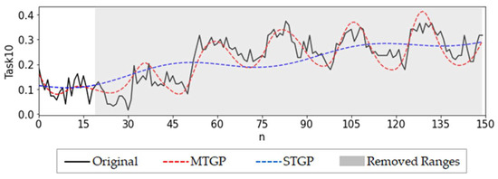
Figure 12.
Imputation results of MTGP and STGP for the extreme situation (after normalization).
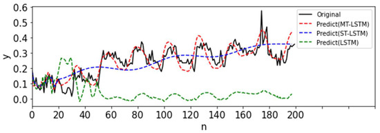
Figure 13.
Prediction results of MT-LSTM, ST-MTGP, and LSTM for the extreme situation (after normalization).
Table 8.
Error results of STGP and MTGP (after normalization).
Table 9.
Error results of MT-LSTM, ST-LSTM, and LSTM (after normalization).
Thereafter, we further performed data pre-processing, such as data denoising and dimensionality reduction; the first five principal components are shown in Figure 14. We found that partial principal components accounted for more information in the original data: the first principal component comprised 73.1%, the second principal component comprised 12.8%, the third principal component comprised 4%, the fourth principal component comprised 3.2%, and the fifth principal component comprised 2.8%. We normalized the first and second principal components (totally accounting for 85.9% of the information in the original data) and integrated them into the MT-LSTM model. The results are shown in Figure 15 and Figure 16, Table 10 and Table 11. We found that the accuracy was significantly high, and the calculation time was about 5 min.
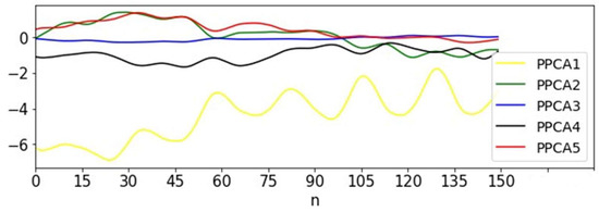
Figure 14.
The first 5 principal components after data pre-processing from the compressor data.
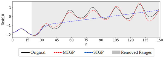
Figure 15.
Imputation results of MTGP and STGP for the extreme situation (with data pre-processing).
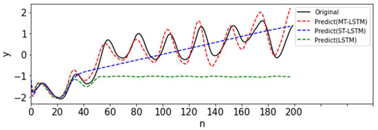
Figure 16.
Prediction results of MT-LSTM, ST-MTGP, and LSTM for the extreme situation (with data pre-processing).
Table 10.
Error results of STGP and MTGP (with data pre-processing).
Table 11.
Error results of MT-LSTM, ST-LSTM, and LSTM (with data pre-processing).
According to the experimental results, it could be found that the LSTM was poor in the scarce-data scenario. For the proposed MT-LSTM model, we performed data imputation of the target task by leveraging knowledge from auxiliary tasks through the modeling of an MTGP and then employed the LSTM to build the sequence model of the target data upon the imputed time-series data to perform a prediction in the future. The knowledge transfer across tasks helps the proposed MT-LSTM perform significantly better than the vanilla LSTM.
4. Conclusions and Discussion
Health management for turbomachinery is a challenging task. Deep learning has gradually entered this industry over the past few years. However, in practical application, the training process of deep learning models requires a large number of samples and time. Due to various reasons, it is difficult to obtain a significant amount of monitoring data, and the health management of turbomachinery has high timeliness and accuracy requirements. To account for the scarce-data scenario in the PHM of turbomachinery, this paper proposes integrating multi-task Gaussian processes, long short-term memory, Bayesian wavelet denoising, and probabilistic principal component analysis to achieve rapid automatic data imputation and time-series modeling to alleviate the need for big data as well as improve predictions with scarce data. Meanwhile, the framework can solve the optimization cleaning of the original multivariate time-series monitoring data, conduct the possible correlation and uncertainty in the multivariate data, and reduce the reliance on professional knowledge and experience. The experimental results show that the proposed method can accurately and efficiently reconstruct and predict with scarce time-series data via multi-task modeling. The superiority of our method is especially obvious for real centrifugal compressor operation data. When there are only 10~20 data points, the proposed method still has high prediction accuracy. This is significant to the prognostics and health management (PHM) of turbomachinery.
Due to the high precision requirement of turbomachinery operation, a slight error may lead to serious accidents; thus, the model’s accuracy should be improved. The main links of the model—data denoising, dimensionality reduction, and MT-LSTM—are processed separately, which is inconvenient for practical application. At present, the model has only been verified by an actual compressor, which cannot effectively investigate its robustness and universality. In fact, large engineering applications usually have hundreds of different types of turbines, and the working conditions are very complex. Therefore, in the future, we will carry out the robustness and universality verification of the model under multiple scenarios, such as multisource data fusion, different turbomachinery types, and different working conditions. In addition, we would like to continue development work in visualization and human–computer interaction in the future.
Author Contributions
Conceptualization, X.C., X.W. and H.L.; methodology, X.C., H.L., Y.Z. and C.L.; software, X.C., H.L., Y.Z. and C.L.; validation, X.C.; formal analysis, X.C.; investigation, X.D. and K.C.; resources, X.D. and K.C.; data curation, X.C.; writing—original draft preparation, X.C. and H.L.; writing—review and editing, X.C., X.D., X.W. and H.L.; visualization, X.C.; supervision, X.W. and H.L.; project administration, X.D. and X.W.; funding acquisition, X.W. and H.L. All authors have read and agreed to the published version of the manuscript.
Funding
This research was funded by the National Natural Science Foundation of China, grant number 52005074; the Natural Science Foundation of Liaoning Province, grant number 2022-MS-135; and the Fundamental Research Funds for the Central Universities, grant number DUT19RC(3)070.
Data Availability Statement
Not applicable.
Conflicts of Interest
The authors declare no conflict of interest.
References
- Insun, S.; Junmin, L.; Young, L.J.; Kyusung, J.; Daeil, K.; Youn, B.D.; Soo, J.H.; Joo-Ho, C. A Framework for Prognostics and Health Management Applications toward Smart Manufacturing Systems. Int. J. Precis. Eng. Manuf. Green Technol. 2018, 5, 535–554. [Google Scholar]
- Lee, G.Y.; Kim, M.; Quan, Y.J.; Kim, M.S.; Kim, T.; Yoon, H.S.; Min, S.; Kim, D.H.; Mun, J.W.; Oh, J.W. Machine health management in smart factory: A review. J. Mech. Sci. Technol. 2018, 32, 987–1009. [Google Scholar] [CrossRef]
- Kalgren, P.W.; Byington, C.S.; Roemer, M.J. Defining PHM, A Lexical Evolution of Maintenance and Logistics. In Proceedings of the 2006 IEEE Autotestcon, Anaheim, CA, USA, 18–21 September 2016. [Google Scholar]
- Sun, C.; Bisland, S.G.; Nguyen, K.; Long, V. Prognostic/Diagnostic Health Management System (PHM) for Fab Efficiency. In Proceedings of the IEEE Advanced Semiconductor Manufacturing Conference, Boston, MA, USA, 22–24 May 2006. [Google Scholar]
- Cui, L.; Huang, J.; Zhang, F.; Chu, F. HVSRMS localization formula and localization law: Localization diagnosis of a ball bearing outer ring fault. Mech. Syst. Signal Process. 2019, 120, 608–629. [Google Scholar] [CrossRef]
- Lc, A.; Jing, W.A.; Sl, B. Matching pursuit of an adaptive impulse dictionary for bearing fault diagnosis. J. Sound Vib. 2014, 333, 2840–2862. [Google Scholar]
- Lei, Y.; Yang, B.; Jiang, X.; Jia, F.; Nandi, A.K. Applications of machine learning to machine fault diagnosis: A review and roadmap. Mech. Syst. Signal Process. 2020, 138, 106587. [Google Scholar] [CrossRef]
- Van, M.; Hoang, D.T.; Kang, H.J. Bearing Fault Diagnosis Using a Particle Swarm Optimization-Least Squares Wavelet Support Vector Machine Classifier. Sensors 2020, 20, 3422. [Google Scholar] [CrossRef]
- Xiong, J.; Zhang, Q.; Peng, Z.; Sun, G.; Xu, W.; Wang, Q. A Diagnosis Method for Rotation Machinery Faults Based on Dimensionless Indexes Combined with K- Nearest Neighbor Algorithm. Math. Probl. Eng. 2017, 2017, 60572929. [Google Scholar] [CrossRef]
- Saini, M.K.; Aggarwal, A. Detection and diagnosis of induction motor bearing faults using multiwavelet transform and naive Bayes classifier. Int. Trans. Electr. Energy Syst. 2018, 28, 115597668. [Google Scholar] [CrossRef]
- Jiang, G.; He, H.; Yan, J.; Xie, P. Multiscale Convolutional Neural Networks for Fault Diagnosis of Wind Turbine Gearbox. IEEE Trans. Ind. Electron. 2019, 66, 3196–3207. [Google Scholar] [CrossRef]
- Lecun, Y.; Bengio, Y.; Hinton, G. Deep learning. Nature 2015, 521, 436. [Google Scholar] [CrossRef]
- Zhang, L.; Gao, H.; Wen, J.; Li, S.; Liu, Q. A deep learning-based recognition method for degradation monitoring of ball screw with multi-sensor data fusion. Microelectron. Reliab. 2017, 75, 215–222. [Google Scholar] [CrossRef]
- Li, C.; Sanchez, R.V.; Zurita, G.; Cerrada, M.; Cabrera, D.; Vasquez, R.E. Gearbox fault diagnosis based on deep random forest fusion of acoustic and vibratory signals. Mech. Syst. Signal Process. 2016, 76–77, 283–293. [Google Scholar] [CrossRef]
- Han, Y.; Tang, B.; Deng, L. An enhanced convolutional neural network with enlarged receptive fields for fault diagnosis of planetary gearboxes. Comput. Ind. 2019, 107, 50–58. [Google Scholar] [CrossRef]
- Han, Y.; Tang, B.; Lei, D. Multi-level wavelet packet fusion in dynamic ensemble convolutional neural network for fault diagnosis. Measurement 2018, 127, 246–255. [Google Scholar] [CrossRef]
- Mei, Y.; Wu, Y.; Li, L. Fault diagnosis and remaining useful life estimation of aero engine using LSTM neural network. In Proceedings of the IEEE International Conference on Aircraft Utility Systems, Beijing, China, 10–12 October 2016. [Google Scholar]
- Jia, F.; Lei, Y.; Lin, J.; Zhou, X.; Lu, N. Deep neural networks: A promising tool for fault characteristic mining and intelligent diagnosis of rotating machinery with massive data. Mech. Syst. Signal Process. 2016, 72, 303–315. [Google Scholar] [CrossRef]
- Shi, J.; He, Q.; Wang, Z. An LSTM-based severity evaluation method for intermittent open faults of an electrical connector under a shock test. Measurement 2020, 173, 108653. [Google Scholar] [CrossRef]
- Chen, L.; Wang, Z.Y.; Qin, W.L.; Ma, J. Fault diagnosis of rotary machinery components using a stacked denoising autoencoder-based health state identification. Signal Process. 2017, 130, 377–388. [Google Scholar]
- Zhao, R.; Yan, R.; Wang, J.; Mao, K. Learning to Monitor Machine Health with Convolutional Bi-Directional LSTM Networks. Sensors 2017, 17, 273. [Google Scholar] [CrossRef]
- Wang, J.; Li, S.; An, Z.; Jiang, X.; Qian, W.; Ji, S. Batch-normalized deep neural networks for achieving fast intelligent fault diagnosis of machines. Neurocomputing 2019, 329, 53–65. [Google Scholar] [CrossRef]
- Guo, X.; Lu, K.; Cheng, Y.; Zhao, W.; Wu, H.; Li, D.; Li, J.; Yang, S.; Zhang, Y. Research on fault diagnosis method for hydraulic system of CFETR blanket transfer device based on CNN-LSTM. Fusion Eng. Des. 2022, 185, 113321. [Google Scholar] [CrossRef]
- Lim, S.L.H.; Duong, P.L.T.; Park, H.; Raghavan, N. Expedient validation of LED reliability with anomaly detection through multi-output Gaussian process regression. Microelectron. Reliab. 2022, 138, 114624. [Google Scholar] [CrossRef]
- Jia, F.; Lei, Y.; Lu, N.; Xing, S. Deep normalized convolutional neural network for imbalanced fault classification of machinery and its understanding via visualization. Mech. Syst. Signal Process. 2018, 110, 349–367. [Google Scholar] [CrossRef]
- Shao, H.; Jiang, H.; Lin, Y.; Li, X. A novel method for intelligent fault diagnosis of rolling bearings using ensemble deep auto-encoders. Mech. Syst. Signal Process. 2018, 102, 278–297. [Google Scholar] [CrossRef]
- Mao, W.; Liu, Y.; Ding, L.; Li, Y. Imbalanced Fault Diagnosis of Rolling Bearing Based on Generative Adversarial Network: A Comparative Study. IEEE Access 2019, 7, 9515–9530. [Google Scholar] [CrossRef]
- Qin, Y.; Wang, X.; Zou, J. The Optimized Deep Belief Networks With Improved Logistic Sigmoid Units and Their Application in Fault Diagnosis for Planetary Gearboxes of Wind Turbines. IEEE Trans. Ind. Electron. 2019, 66, 3814–3824. [Google Scholar] [CrossRef]
- Zhuang, Z.; Qin, W. Intelligent fault diagnosis of rolling bearing using one-dimensional Multi-Scale Deep Convolutional Neural Network based health state classification. In Proceedings of the ICNSC 2018, Zhuhai, China, 27–29 March 2018. [Google Scholar]
- Rasmussen, C.E.; Williams, C. Gaussian Processes for Machine Learning. In Gaussian Processes for Machine Learning; The MIT Press: London, MA, USA, 2005. [Google Scholar]
- Lvarez, M.A.; Luengo, D.; Titsias, M.K.; Lawrence, N.D. Efficient Multioutput Gaussian Processes through Variational Inducing Kernels. JMLR Workshop Conf. Proc. 2010, 9, 25–32. [Google Scholar]
- Osborne, M.A.; Roberts, S.J.; Rogers, A.; Jennings, N.R. Real-time information processing of environmental sensor network data using Bayesian Gaussian processes. ACM Trans. Sens. Netw. 2012, 9, 1–32. [Google Scholar] [CrossRef]
- Skolidis, G. Bayesian Multitask Classification With Gaussian Process Priors. IEEE Press 2011, 22, 2011–2021. [Google Scholar] [CrossRef]
- Zhou, X.; Qin, T.; Ji, M.; Qiao, D. A LSTM assisted orbit determination algorithm for spacecraft executing continuous maneuver. Acta Astronaut. 2022; in press. [Google Scholar] [CrossRef]
- Hu, C.; Zhao, Y.; Jiang, H.; Jiang, M.; You, F.; Liu, Q. Prediction of ultra-short-term wind power based on CEEMDAN-LSTM-TCN. Energy Rep. 2022, 8, 483–492. [Google Scholar] [CrossRef]
- Liu, X.; Zhou, Q.; Zhao, J.; Shen, H.; Xiong, X. Fault Diagnosis of Rotating Machinery under Noisy Environment Conditions Based on a 1-D Convolutional Autoencoder and 1-D Convolutional Neural Network. Sensors 2019, 19, 972. [Google Scholar] [CrossRef]
- Ewees, A.A.; Al-qaness, M.A.A.; Abualigah, L.; Elaziz, M.A. HBO-LSTM: Optimized long short term memory with heap-based optimizer for wind power forecasting. Energy Convers. Manag. 2022, 268, 116022. [Google Scholar] [CrossRef]
- Durichen, R.; Davenport, L.; Bruder, R.; Wissel, T.; Ernst, F. Evaluation of the potential of multi-modal sensors for respiratory motion prediction and correlation. In Proceedings of the Conference International Conference of the IEEE Engineering in Medicine & Biology Society IEEE Engineering in Medicine & Biology Society Conference, Osaka, Japan, 3–7 July 2013. [Google Scholar]
Disclaimer/Publisher’s Note: The statements, opinions and data contained in all publications are solely those of the individual author(s) and contributor(s) and not of MDPI and/or the editor(s). MDPI and/or the editor(s) disclaim responsibility for any injury to people or property resulting from any ideas, methods, instructions or products referred to in the content. |
© 2022 by the authors. Licensee MDPI, Basel, Switzerland. This article is an open access article distributed under the terms and conditions of the Creative Commons Attribution (CC BY) license (https://creativecommons.org/licenses/by/4.0/).