Article

A Surface Defect Inspection Model via Rich Feature Extraction and Residual-Based Progressive Integration CNN

1
School of Mechanical Engineering, Suzhou University of Science and Technology, Suzhou 215000, China
2
College of Mechanical and Electrical Engineering, Shihezi University, Shihezi 832061, China
*
Author to whom correspondence should be addressed.
Machines 2023, 11(1), 124; https://doi.org/10.3390/machines11010124
Submission received: 16 December 2022 / Revised: 13 January 2023 / Accepted: 13 January 2023 / Published: 16 January 2023

Abstract

:
Surface defect inspection is vital for the quality control of products and the fault diagnosis of equipment. Defect inspection remains challenging due to the low level of automation in some manufacturing plants and the difficulty in identifying defects. To improve the automation and intelligence levels of defect inspection, a CNN model is proposed for the high-precision defect inspection of USB components in the actual demands of factories. First, the defect inspection system was built, and a dataset named USB-SG, which contained five types of defects—dents, scratches, spots, stains, and normal—was established. The pixel-level defect ground-truth annotations were manually marked. This paper puts forward a CNN model for solving the problem of defect inspection tasks, and three strategies are proposed to improve the model’s performance. The proposed model is built based on the lightweight SqueezeNet network, and a rich feature extraction block is designed to capture semantic and detailed information. Residual-based progressive feature integration is proposed to fuse the extracted features, which can reduce the difficulty of model fine-tuning and improve the generalization ability. Finally, a multi-step deep supervision scheme is proposed to supervise the feature integration process. The experiments on the USB-SG dataset prove that the model proposed in this paper has better performance than that of other methods, and the running speed can meet the real-time demand, which has broad application prospects in the industrial inspection scene.

1. Introduction

Defect detection is an important part of a product’s quality control [1,2]; more and more manufacturers are paying more attention to the surface quality of products and have put forward more stringent requirements. The purpose of surface defect detection is to find whether defects on the surfaces of products are related to functional defects and the aesthetics of products. Defects will affect product yield, resulting in reduced production efficiency and waste of raw materials. In addition, a product’s surface defects will affect users’ intuitive feeling. Defects in some critical facilities, such as vehicles, buildings, precision equipment, etc., may lead to severe economic losses and casualties. Good product quality is an essential prerequisite for manufacturers to achieve a high market share. Many enterprises still rely on human resources for product surface quality inspection. Depending on human resources will not only bring an economic burden to enterprises, but efficiency and accuracy cannot be guaranteed. Heavy work will also harm the health of workers. Therefore, it is of great significance to propose a scheme that can replace human resources and realize automatic and intelligent defect inspection tasks [3].
With the rapid development of information technology, machine vision has been applied in many industrial production and inspection fields, including those of fabrics [4], glass [5], multicrystalline solar wafers [6], and steel [7]. In order to solve the above problems, researchers have proposed detection methods from various aspects. Song, K. et al. proposed a feature descriptor template named AECLBPs in a steel surface inspection system [7]. K. L. Mak proposed a novel defect detection scheme based on morphological filters for automated defect detection in woven fabrics [8]. X. Kang et al. proposed a universal and adaptive fabric defect detection algorithm based on sparse dictionary learning [9]. Lucia, B. et al. proposed a feature extraction phase by using Gabor Filters and PCA for texture defect feature detection [10]. These defect feature extractors were artificially designed, and researchers could quickly select the defect feature extractors according to their experience. Therefore, defect detection performance depends heavily on manually defined defect feature representations. New changes in the feature morphologies of defects will lead to a reduction in the defect recognition performance [11].
In the last decade, due to the rapid development of the Internet, big data, and the computing equipment industry, convolutional neural networks (CNNs) have become a new trend for machine-vision-related tasks [12]. Due to the computing power of convolutional neural networks, they are trained on large amounts of data. A CNN can allow artificially designed feature extractors to be avoided and can automatically learn a large number of useful detailed and semantic features. Therefore, a network model can obtain good generalization performance. CNNs have been applied to many research fields, such as object detection [13,14], human posture recognition [15], super-resolution [16], autonomous driving [17], etc.
These findings have inspired researchers to apply CNNs to vision-based industrial inspection tasks. CNN-based defect inspection tasks can be divided into two categories: defect classification and defect localization.
(1) Defect classification approaches: Yi Li et al. proposed an end-to-end surface defect recognition system that was constructed by using the symmetric surround saliency map and a CNN [18]. Fu et al. proposed a defect classification CNN model, which emphasized the training of low-level features and incorporated multiple receptive fields to achieve fast and accurate steel surface defect classification [11]. T. Benbarrad et al. studied the impact of image compression on the classification performance of steel surface defects with a CNN [19]. Myeongso Kim et al. proposed a CNN-based transfer learning method for defect classification in semiconductor manufacturing [20].
(2) Defect localization approaches: Unlike in defect classification, defect location can provide specific location information of defects in the detected target, which is a task requiring a higher accuracy of defect identification. Ren et al. presented a CNN model for performing surface defect inspection tasks, and feature transferal from pre-trained models was used in the model [21]. T Wang et al. proposed a CNN model for product quality control [22]. Mei Zhang et al. proposed a one-class classifier for image defect detection [23]. Yibin Huang et al. proposed a compact CNN model for surface defect inspection, and the model consisted of a lightweight (LW) bottleneck and a decoder [24]. D. Tabernik et al. proposed a segmentation-based CNN model for segmenting surface anomalies [25]. Saliency detection aims to detect the most interesting object in an image [26,27,28,29,30], which is close to the target of defect inspection. Yibin Huang et al. proposed a deep hierarchical structured convolutional network for detecting magnetic tile surface defect saliency [31].
In the construction of a defect location model, to obtain the location information of defects, it is necessary to combine an encoder and decoder and fuse low-level features in the decoding process to generate a higher-resolution feature map. Designing a more effective feature extraction and fusion architecture is a hot research direction for defect location. U-Net is a widely used encoder–decoder architecture [32], and it was first applied to biomedical image segmentation. A typical U-Net structure consists of a contracting path to capture semantic context information and a symmetric expanding path that enables precise localization. Inspired by this structure, many researchers have designed similar architectures for the defect inspection task.
Semantic information is crucial in object recognition tasks, including defect localization, which is related to the physical meaning of the target. Semantic information is richer in a convolutional neural network’s deeper layer. On the contrary, the shallow layer has weaker semantic information. Some existing methods have built models by designing decoder structures based on high-level semantic features [24,25]. On this basis, some researchers used these semantic features at individual scales to create a decoder structure. Researchers have paid little attention to features with weaker semantic information at the individual scale. It is worth noting that these features have more detailed information, and they are helpful clues for capturing accurate defect location information. In addition, some existing defect localization CNN models do not use high-level semantic and detailed low-level features well.
To settle these problems, we propose a novel CNN model for obtaining fast and accurate pixel-level defect localization. Our model is constructed on a pre-trained lightweight SqueezeNet model. We propose three effective techniques for achieving the effective extraction of semantic and detailed information, fusion, and supervision. The proposed model is applied to our defect inspection system. To verify the validity of this model, a pixel-level defect dataset, USB-SG, was collected and labeled in this paper, and it contained a total of 683 images with five defect types. Comparative experiments verify the effectiveness and superiority of the proposed model. The proposed model runs at a speed of over 30 FPS when processing 200 × 200 images on an NVIDIA 1080TI GPU, which could satisfy the demand for a real-time defect inspection task. The main contributions of this paper can be summarized as follows:
  • To improve the automation and intelligence levels of defect inspection, this paper proposes a defect inspection system based on a CNN. The proposed model is built based on a lightweight SqueezeNet model.
  • We design three effective techniques to improve the performance of the proposed model. Firstly, rich feature extraction blocks are used to capture both semantic and detailed information at different scales. Then, a residual-based progressive feature fusion structure is used to fuse the extracted features at different scales. Finally, the fusion results of defects are supervised in multiple fusion steps.
  • To verify the effectiveness of the proposed model, we manually labeled a pixel-level defect dataset, USB-SG, which included markings of the defect locations. The dataset included five defect types—dents, scratches, spots, stains, and normal—with a total of 684 images.
  • Our approach could obtain higher detection accuracy compared with that of other machine learning and deep-learning-based methods. The running speed of this model was able to reach real time, and it has wide application prospects in industrial inspection tasks.
The rest of this paper is organized as follows. In Section 2, the defect inspection system and proposed dataset are introduced. The proposed method is introduced in Section 3. The implementation details, ablation study, and experimental comparisons of our proposed model are presented in Section 4. Finally, Section 5 concludes the paper.

2. Defect Inspection System and Proposed Dataset

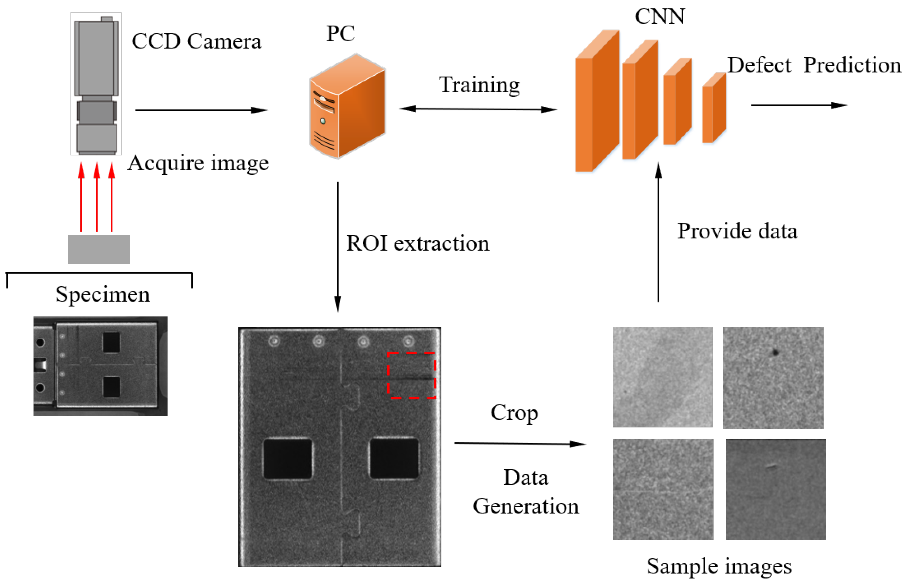
This section presents the details of the defect inspection system and proposed dataset. The complete structure of the proposed model is shown in Figure 1.

2.1. Defect Inspection System

The defect detection system proposed in this paper is intended to solve the actual product defect requirements of production plants. The core of the defect inspection system is the design of a high-performance defect inspection model that can find possible defect areas on the surfaces of products and further obtain visual and digital surface quality monitoring results. The defect inspection system was set up to acquire workpiece surface defect images, as shown in Figure 1. The hardware configuration included the inspected specimens, light sources, CCD cameras, a lens, computers, etc. The sample to be tested here was the universal serial bus (USB) connector. Since this part undergoes cutting, bending, and other machining methods during the production process, there may be various types of defects on the surface, which will affect the product’s quality. Considering the small physical size of the defects—with some being even less than 0.5 mm—a 2448 × 2048 resolution monochrome industrial camera was used to obtain high-resolution images of defects. To build the image acquisition system, it was necessary to adjust the distance between the camera lens and the specimen and to select the appropriate light source type and angle. In the process of the experimental setup, these components needed to be adjusted to obtain the best sample surface recognition effect and, in particular, to highlight the defect characteristics.
The image data recorded by the camera were transferred to a computer for processing. Extraction of regions of interest (ROIs) was carried out on the obtained images; the background region was removed, while the specimen region was retained. In order to facilitate unified processing, all of the sample sizes were adjusted to 800 × 1000. Cropping is a common data augmentation technique that has been applied in various defect inspection tasks [33,34]. In addition, there were two limitations to our defect inspection task. Firstly, the number of defect samples was insufficient. Secondly, the size of many defects was tiny, and it would be difficult to identify small defects if the resolution of the input image was compressed. If the ROI image was input into the network with a resolution of 800 × 1000, the operation efficiency of the network would be reduced. Based on the above considerations, the ROI image was not directly used as the input image, and we cropped 200 × 200 resolution image patches from the ROI image. In order to obtain valid defect samples, the defective regions would be cropped. The generated defect image dataset was trained on the proposed model by using a PC equipped with a GPU, and the model could predict defective areas after training.

2.2. Pixel-Level USB-SG Defect Dataset

The dataset proposed in this paper was named USB-SG, and each sample in the dataset was composed of an original image and the corresponding ground-truth map. In the ground-truth map, the position of the defect was manually marked as the foreground. The USB-SG dataset included five types of image samples: dented, scratched, spotted, stained, and normal samples (defect-free). Some samples of all defect types and their ground-truth maps are shown in Figure 2.
It should be noted that the four types of defects had their own characteristics. Dents appeared as small and deep indentations; scratches appeared as slender traces; spots appeared as round or oval color attachments; stains appeared as large areas of lil or other materially affected areas. It was observed that the size and morphology of the different types varied, such as those of dents and stains. It is worth noting that some defects’ practical physical sizes were quite small—even less than 0.5 mm. Therefore, achieving high-accuracy inspection in the defect dataset was challenging. The purpose of adding normal samples to the dataset was to enable the detection model to learn the topographies of normal regions so as to distinguish between defect and defect-free features. The numbers of the five defect types are given in Table 1. The total numbers of dented, scratched, spotted, stained, and normal samples were 116, 120, 68, 56, and 323, respectively. The whole dataset was then randomly split into a training set and test set. In this way, it was guaranteed that the training and test sets were obtained under the same conditions. This was helpful for improving the performance and reliability of the model in the process of defect testing. The ratio of the training set to the test set was about 80% to 20%.

3. Proposed Method

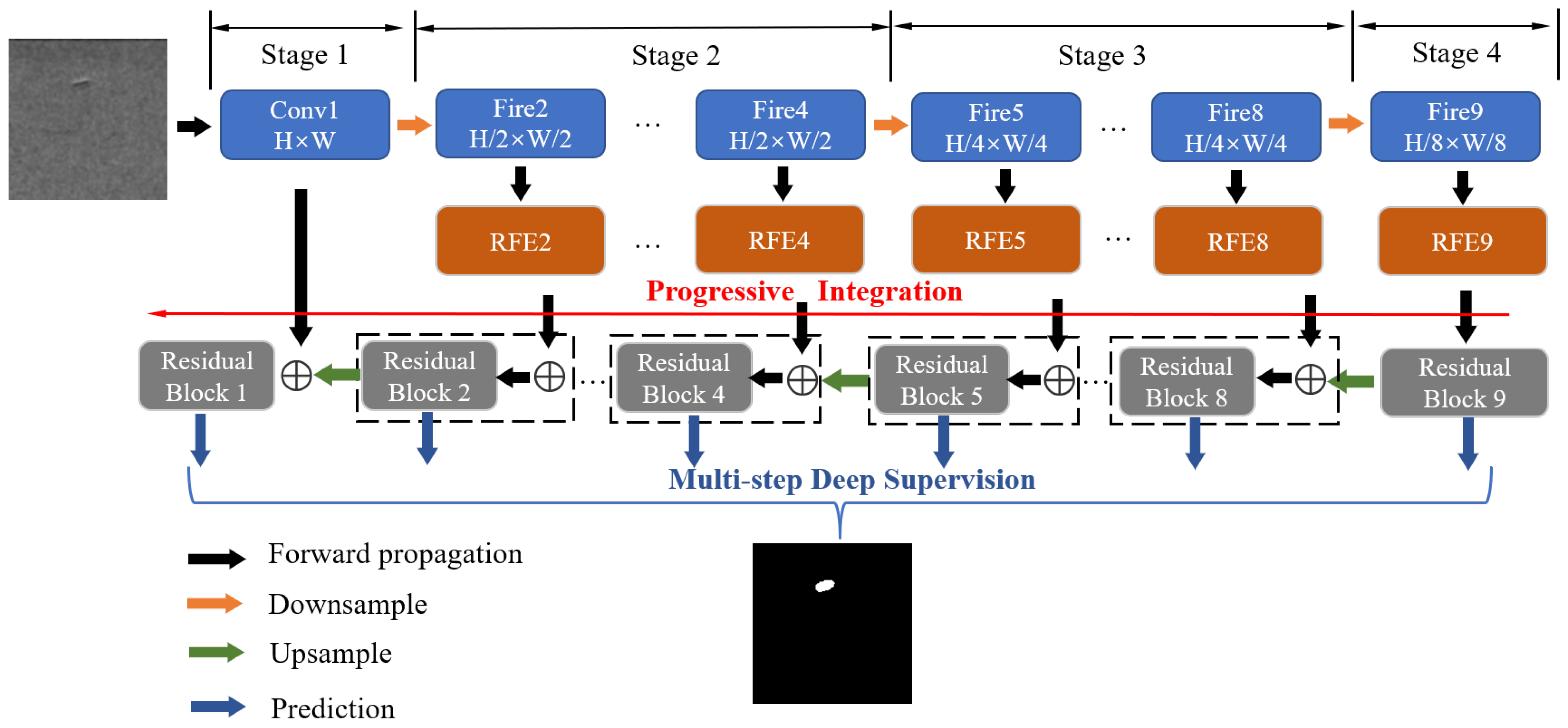
In order to solve the problem of the defect inspection of universal serial bus (USB) connectors, this paper proposes an end-to-end CNN, as shown in Figure 3. The proposed model consisted of three main components, namely, (1) a rich feature extraction (RFE) block, (2) residual-based progressive integration (RPI), and (3) multi-step deep supervision (MsDS). The intrinsic connection of these three parts is as follows: The defect features with semantic information and detailed information at different scales were obtained by the RFE block, and then the extracted features were integrated through the RPI fusion scheme. Furthermore, the fusion process was effectively supervised through the MsDS strategy. The detailed structure and characteristics of each component are presented in the following subsections.

3.1. Rich Feature Extraction

The proposed architecture was constructed based on the lightweight SqueezeNet model. SqueezeNet was proposed by Iandola et al. [35] to keep a good balance between performance and efficiency. The SqueezeNet model consists of a convolution layer and eight Fire modules (Fire 2 ∼ Fire 9). These modules can be divided into four stages based on the scale, as shown in Figure 3. Each single Fire module contains three convolution layers; one is used to compress the number of channels to reduce the parameters, and the other two are used to carry out feature learning and increase the receptive field. We intended to build our convolutional neural network based on the SqueezeNet backbone. Feature extraction is the basis of building convolutional neural networks; a comparison of the different feature extraction strategies is shown in Figure 4.
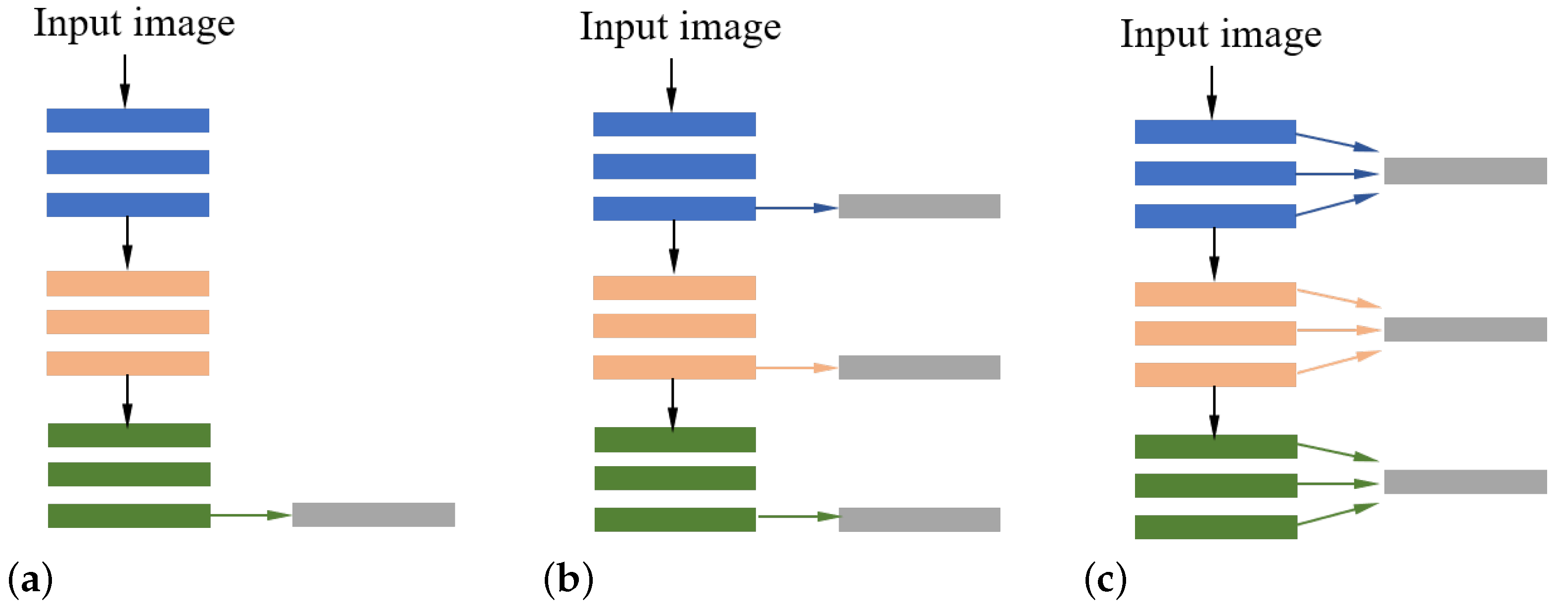
Most existing object localization models have two primary schemes when extracting features from the backbone network, as shown in Figure 4a,b. (a) The last convolution layer feature of the last stage is used, and then the subsequent network structure is designed based on this feature [24,25]. (b) The last convolution layer features at all stages are used [36,37]. These methods extract the feature with the richest semantic information in the backbone network or use the layer with the richest semantic information in each stage to build the model. However, for object localization tasks, the positional accuracy of features is also important. A model’s lower stages have more location-related information, while each stage’s shallower layers contain more information overall. In this paper, we propose a rich feature extraction (RFE) scheme that utilizes convolution layers with semantic and detailed information at all stages. The illustration of the proposed RFE is shown in Figure 4c.
To illustrate how the layers are connected in RFE, the details of the generative process of the proposed RFE block are shown in Figure 5. The Relu activation function is omitted for brevity. The SqueezeNet backbone is composed of one convolutional layer, three pooling layers, and eight Fire modules (Fire 2 9 ). The ith RFE block was built based on the ith Fire module. Fire i/Squeeze, Fire i/Expand 1 × 1, and Fire i/Expand 3 × 3 were the three convolutional layers that constituted the Fire module. The arrows in Figure 5 refer to the input–output relationship between the different layers in the model. For example, Fire i/Expand 1 × 1 and Conv S i are connected to Sum i _ 1 , which indicates that both of them are the inputs of Sum i _ 1 . The left side of Figure 5 shows the relationship between the features and the depth. The shallow layers in the model are the low-level features, and the deep layers are the high-level features. As the layers go deeper, the features contain more semantic features and less detailed information. In the ith Fire module, Fire i/Squeeze is located at a shallower position than those of Fire i/Expand 1 × 1 and Fire i/Expand 3 × 3. Therefore, in order to obtain as rich of information as possible, it is necessary to make use of them all. RFB takes all three convolutional layers as input. Conv S i is used to adjust the channel numbers of Fire i/Squeeze. The summation layer is used to fuse the Conv S i and Fire i/Expand layers. Sum i _ 1 and Sum i _ 3 are followed by Conv i _ 1 and Conv i _ 3 , respectively. Conv i _ 1 and Conv i _ 3 are fused together, and then convoluted by Conv F i to obtain the final output of the ith RFE block.

3.2. Residual-Based Progressive Integration

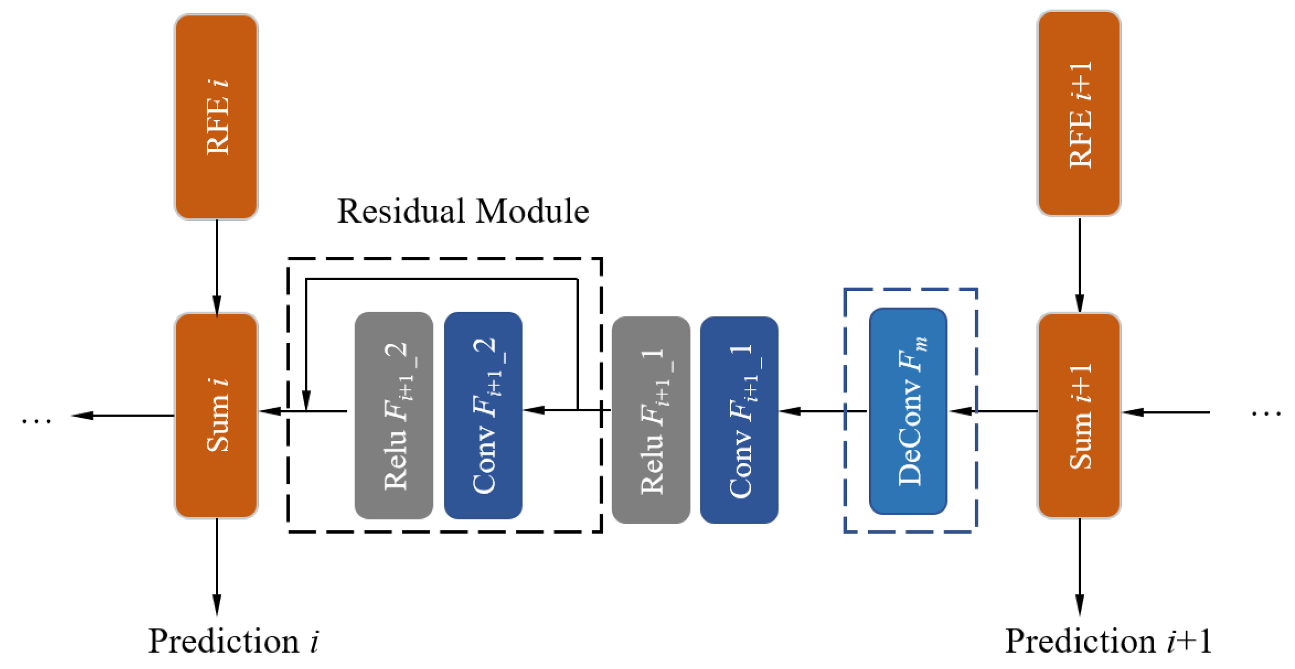
Through the feature extraction block, a series of extracted features were obtained, among which RFE9 was a high-level feature with more semantic information, and RFE2 was a low-level feature with more detailed information. From RFE9 to 2, the semantic information became weaker and the detailed information became stronger. The means of effectively integrating them needs to be explored. Inspired by He [38], a residual-based progressive integration (RPI) scheme is proposed. The illustration of the proposed RPI is shown in Figure 6. The figure shows the details of the feature integration process of the ith RFE and the neighboring i + 1 RFE. It should be noted that when i= 8, 4, and 1, a deconvolution layer (named “DeConv F m ” in Figure 6) is added to improve the scale, and the deconvolution layer doubles the size of the feature map to obtain defect features with a higher resolution. Both the stride and the pad of the deconvolution layers were set to 2. The ith +1 RFE was processed by a convolution layer and a residual module and then summed with the ith RFE, thus feeding into the next integration step. The shortcut connection in the residual module could provide richer paths, which was beneficial for strengthening the gradient back-propagation, reducing the gradient dispersion, and effectively improving the model’s generalization ability. In addition, the proposed RPI was able to realize the progressive optimization process from coarse to fine prediction results and effectively reduce the difficulty of training. The effectiveness of the proposed RPI is provided in Section 4.3.

3.3. Multi-Step Deep Supervision

To promote the efficient fusion of the extracted features, we propose a multi-step deep supervision scheme. Multi-scale supervision [36,37] is better than the most widely used single supervision [24,25] because it can supervise the prediction results on multiple scales. More supervision could accelerate the training and improve the detection performance. It is worth noting that the feature integration process of our network consisted of several steps that do not directly correspond to the scale. Based on the above observations, we put forward a scheme that was different from multi-scale supervision—multi-step deep supervision (MsDS), which can be supervised at each step—and the supervision process was more refined and smooth.
Deconvolution layers were used to connect the fusion features of each step to produce the predicted results. The channel number of the deconvolution layers was 1. The sigmoid function was used to activate the features, and it was defined as
p x ( i ) = 1 1 + e x ( i )
where x ( i ) is the pixel value of the deconvolution layer in the ith prediction branch. The corresponding cross-entropy loss function is defined as
L i = 1 N x ( i ) [ y x ( i ) · log ( p x ( i ) ) + ( 1 y x ( i ) ) · log ( 1 p x ( i ) ) ]
where y x ( i ) is the label of the pixel, y x ( i ) = 1 for the foreground, and y x ( i ) = 0 for the background. N is the total number of image pixels.
The loss of the whole model is defined as
L a l l = i = 1 M α i L i
where α i is the loss weight of individual loss, α i = 1 for i = 1 to M, and M is the total number of supervisions used in the proposed model, which corresponds to the maximum value of i in Figure 6. In order to find the optimal number of loss functions, details of the experiments are provided in Section 4.3.3.

4. Experiments

This section first introduces the details of the experimental setup and the evaluation indicators. An ablation study was conducted in order to verify the effectiveness of the proposed optimization strategy. Fair quantitative comparison experiments were organized to compare the performance with that of other existing detection models, which could demonstrate the superiority of the proposed model.

4.1. Implementation Details

The dataset used in the experiment was USB-SG; detailed information on the training set and test set is shown in Table 1, and no data augmentation techniques were used. All of the experiments are carried out with the same dataset settings. The experiments were implemented on the publicly available Caffe deep learning platform [39]. We chose the stochastic gradient descent (SGD) policy to train the model. The weight decay was set to 10 4 , and the momentum was set to 0.9 . The batch size was set to 16, which meant that 16 sample images were computed per iteration. The base learning rate was set to 0.01. The hardware for the experiments was Intel-i7 CPU and NVIDIA 1080Ti GPU.

4.2. Evaluation Index

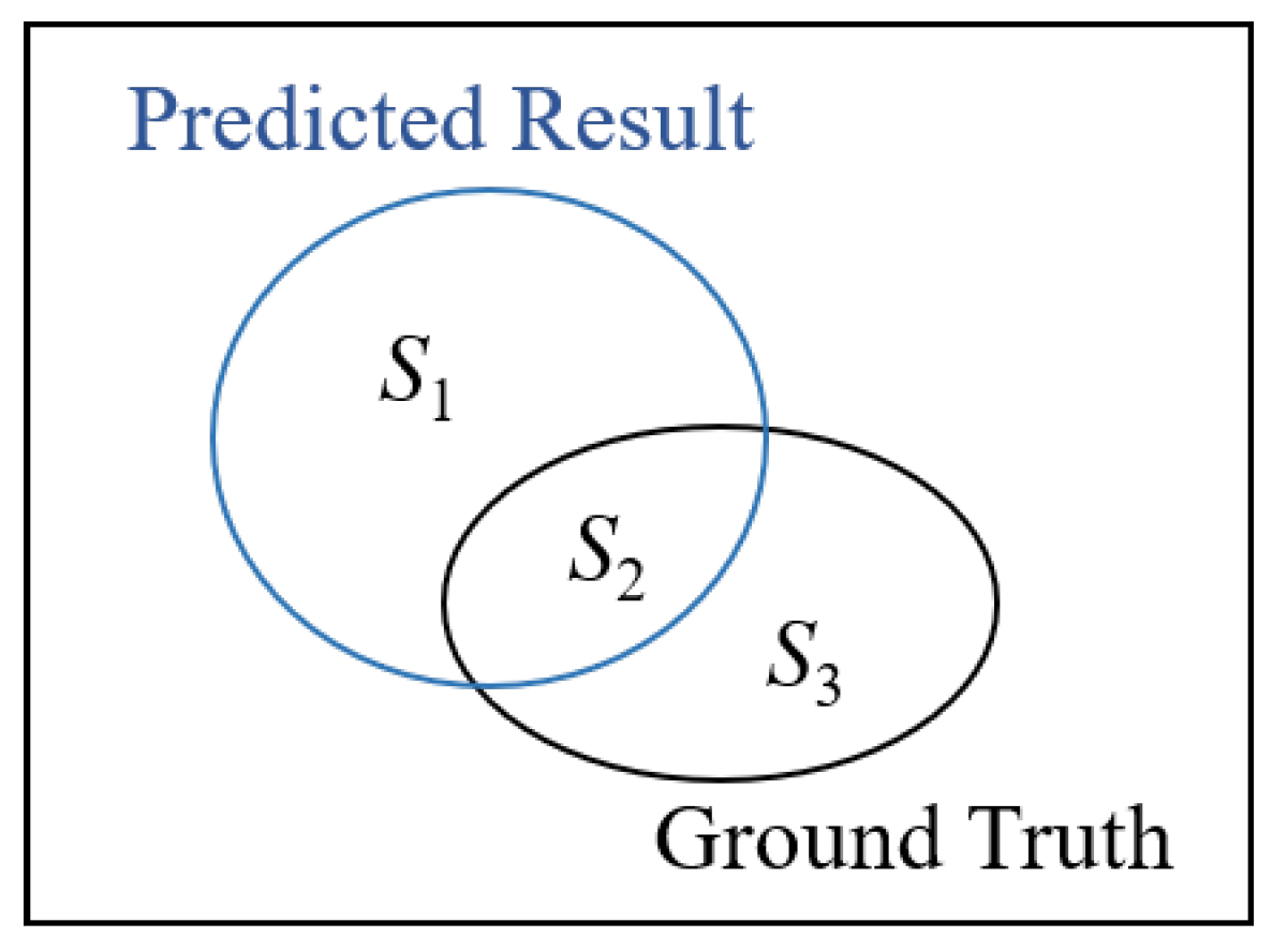
To comprehensively evaluate the performance of the defect location model, four indexes were used to analyze the detection results of the model. They were the precision, recall, F β , mean absolute error (MAE), and Dice coefficient [40]. To better illustrate the calculation process for these indexes, a diagram of the predicted results and ground truth is shown in Figure 7.
S 1 was included in the predicted region, but not included in the ground truth; S 2 was included in both the predicted region and the ground truth; S 3 was included in the ground truth, but not included in the predicted region. The Dice coefficient was defined as
Dice = 2 S 2 / ( S 1 + 2 S 2 + S 3 )
The precision and recall were calculated as
Precision = S 2 / ( S 1 + S 2 )
Recall = S 2 / ( S 2 + S 3 )
Because precision and recall are inversely correlated, precision is generally more important than recall. F β was used to keep a balance between precision and recall, and it was defined as
F β = ( 1 + β 2 ) × Precision × Recall β 2 × Precision + Recall
F β was set to 0.3 in our experiment. The mean absolute error (MAE) was used to measure the difference between the predicted result and the ground truth, and it was defined as
MAE = 1 W × H x = 1 W y = 1 H | S 1 S 3 |
It is noted that the model with the highest F β and lowest MAE had the best performance.

4.3. Ablation Study

In this part, we discuss the three proposed model optimization strategies in detail and organize systematic experiments to verify their effectiveness.

4.3.1. Rich Feature Extraction

The proposed RFE block could extract semantic and detailed information at all stages, which is helpful in accurately capturing the defects. In Section 3.1, we explained the differences between the proposed method and two existing schemes. The experimental comparisons are shown in Table 2. For a fair comparison, all of the models were constructed with the SqueezeNet backbone. It can be seen from the experimental results that the proposed RFE had a higher F β /Dice coefficient and lower MAE-1/MAE-2 than the other two schemes (SQ-a and SQ-b). It can be concluded that the proposed RFE block was more effective than the other two existing schemes.

4.3.2. Residual-Based Progressive Integration

To explore the effectiveness of RPI, two pairs of comparisons are conducted. The experimental comparisons are shown in Table 3. Firstly, a widely used feature fusion method, Unet [32] (SQ-Unet), was compared with our SQ-RPI. The experimental results showed that RPI could achieve higher values of F β (0.6781 vs. 0.6340) and the Dice coefficient (0.6515 vs. 0.6057) and a lower MAE (0.0170 vs. 0.0174, 0.0090 vs. 0.0094). Through the experimental results of the second pair, it could be found that, on the basis of the proposed SQ-RFE model, the addition of RPI could improve F β (0.6862 vs. 0.6702) and the Dice coefficient (0.6640 vs. 0.6484) and could decrease the MAE (0.0158 vs. 0.0167, 0.0084 vs. 0.0088). Through the comparative experiment on the two different baseline models (SQ-Unet and SQ-RFE), it could be concluded that the proposed RPI was effective and robust. In addition, it was proved that the structure of RPI had a good generalization ability and can be applied to similar tasks.

4.3.3. Multi-Step Deep Supervision

In order to analyze the influence of MsDS on the model performance and find the optimal amount of supervision, a series of comparative experiments were organized, and they are shown in Table 4. First, the model performance of SQ-REF-RPI without MsDS was compared with that of SQ-REF-RPI-MsDS. Then, comparisons of the model performance of SQ-REF-RPI-MsDS with different amounts of supervision M are provided.
It was observed that the application of MsDS on SQ-RFE-RPI improved the performance, even with different amounts of supervision. In more detail, the model performed best when the amount of supervision was M = 5 . As the amount of supervision M increased, the performance tended to deteriorate. It should be noted that the features of the last predictions (predictions 9, 8, and 7) contained less detailed information; thus, they had a greater difference from the ground truth. Paying more attention to the coarse predictions in the training process will affect the performance of other predictions.
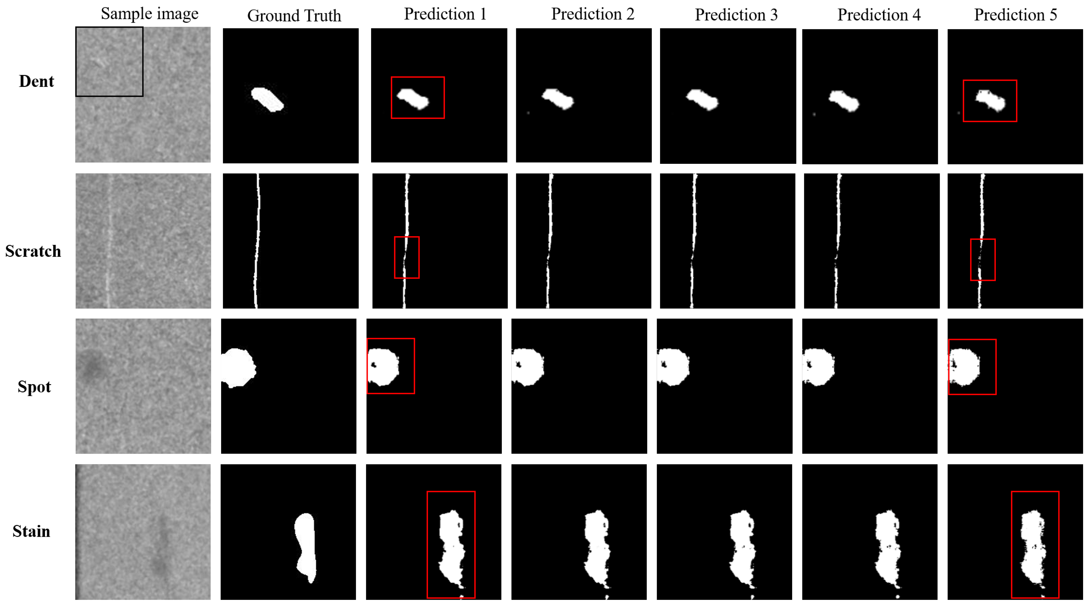
The above experimental results confirmed that the performance was best when there were five supervisions in the model. In order to analyze the relationship between the different predictions, five different predictions were computed, as shown in Table 5. It was observed that from P 5 to P 1 , F β and the Dice coefficient increased, and the MAE decreased. This was because P 1 had the most abundant semantic information and most detailed information, which indicated that the process of learning defect features in the model was from coarse to refined.
In addition to the quantitative analysis, visual comparison experiments for different predictions were conducted, as shown in Figure 8. All four defect types were compared to make the experiments more comprehensive. The first row contains dent-type defects. It was observed that from Prediction 5 to 1, the defective regions became integral, the holes were reduced, and the edges became smoother. A similar situation can be observed in the third and fourth rows. The second row contains scratch-type defects, whose characteristic morphology is slender stripes. From Prediction 5 to 1, it was noted that the disconnected part was gradually connected so that the defect region became complete. In conclusion, the proposed model could provide more accurate predictions by using RPI to integrate semantic and detailed information.

4.3.4. Loss Function

In our model, we chose the most commonly used cross-entropy as our loss function. In recent years, the loss function has also been a hot topic for researchers. Xiaoya Li et al. proposed Dice loss to associate training examples with dynamically adjusted weights to de-emphasize easy-negative examples [41]. The Dice loss is defined as
D L i = 1 2 p x y x + b p x 2 + y x 2 + b
where b indicates the weights, and it is usually set to 1; the rest of the variables were mentioned in Section 3.3.
K. He et al. proposed focal loss [42]. When an image contains a large number of negative data samples, most of the loss and gradient will be dominated by negative samples. Focal loss prevents the vast number of easy negatives from overwhelming the detector during training. The focal loss is defined as
F L i = 1 N x a [ y x γ · log ( p x ) + ( 1 y x ) γ · log ( 1 p x ) ]
where a and γ are the weights, and the rest of the variables were mentioned in Section 3.3.
To explore the influence of the above two loss functions on the proposed model, we conducted comparative experiments while using different loss functions. The setup was the same for all experiments, except for the loss function. The experimental results are shown in Table 6. Cross-entropy was adopted as the loss function in the proposed model due to its stability and trainability. Dice loss was implemented by using the default parameter, and focal loss was adopted with two sets of parameters: (1) a = 1 and γ = 0.5 ; (2) a = 1 and γ = 2 . From the experimental results, it could be found that the performance when using Dice loss was slightly lower than that when using cross-entropy. Focal loss (setting a = 1 and γ = 0.5 ) achieved better performance than that of cross-entropy; when a = 1 and γ = 2 , the performance became worse. This was because setting an appropriate weight in focal loss, such as a = 1 and γ = 0.5 , could suppress the loss of negative samples and enhance the learning effect of positive samples. In the future, focal loss can be applied to the proposed model to boost the defect detection performance.

4.4. Comparisons with Other Models

To verify the effectiveness of the proposed model, we compared our model with other defect/object localization models. To make the experimental comparison more comprehensive, traditional non-deep learning (DL)-based and DL-based methods were included. The non-DL-based methods included AC [27], BMS [28], FT [43], GMR [44], HC [29], LC [45], MBP [46], MSS [47], PHOT [48], RC [29], Rudinac [49], SF [30], and SR [50]. The deep-learning-based methods included the widely used U-Net [32], Rec [51], SegNet [52], and LPBF-Net [53]. All of the experimental results were either reproduced from the source code provided by the authors or implemented based on the original article. A comparative evaluation of the different defect/object localization models on USB-SG defect dataset is shown in Table 7.
These non-DL-based methods used hand-crafted feature extractors to realize object detection/localization tasks. Among these artificial design feature extraction methods, Rudinac, SF, and SR were the three best methods, as they had the highest F β and the lowest MAE. It was observed that the F β values of almost all non-DL-based methods were around 0.2, and the MAE values were around 0.05 0.1 . It could be concluded that the performance of most of the detection methods was very poor, and these methods were not adequate for the task of defect inspection. The reason behind this was that these methods were based on hand-crafted feature extractors, which had a certain subjectivity. As a result, the generalization ability and robustness of the models were limited. These deep-learning-based methods (U-Net, Rec, SegNet, and LPBF-Net) performed better than the methods mentioned above. U-Net is a very influential model that has been widely used in many fields and scenes. Through the experimental comparison, it could be found that the model proposed in this paper had higher F β values (0.7057 vs. 0.6388 vs. 0.6883 vs. 0.6862 vs. 0.6968), lower MAE (0.0151 vs. 0.0183 vs. 0.0162 vs. 0.0160 vs. 0.0157, 0.0080 vs. 0.0098 vs. 0.0085 vs. 0.0084 vs. 0.0082 ) and higher Dice coefficient values (0.6854 vs. 0.6217 vs. 0.6789 vs. 0.6797 vs 0.6806) than those of the other two deep learning models. This was because this paper designed a proper defect feature extraction, integration, and supervision scheme that can accomplish high-precision defect detection tasks.
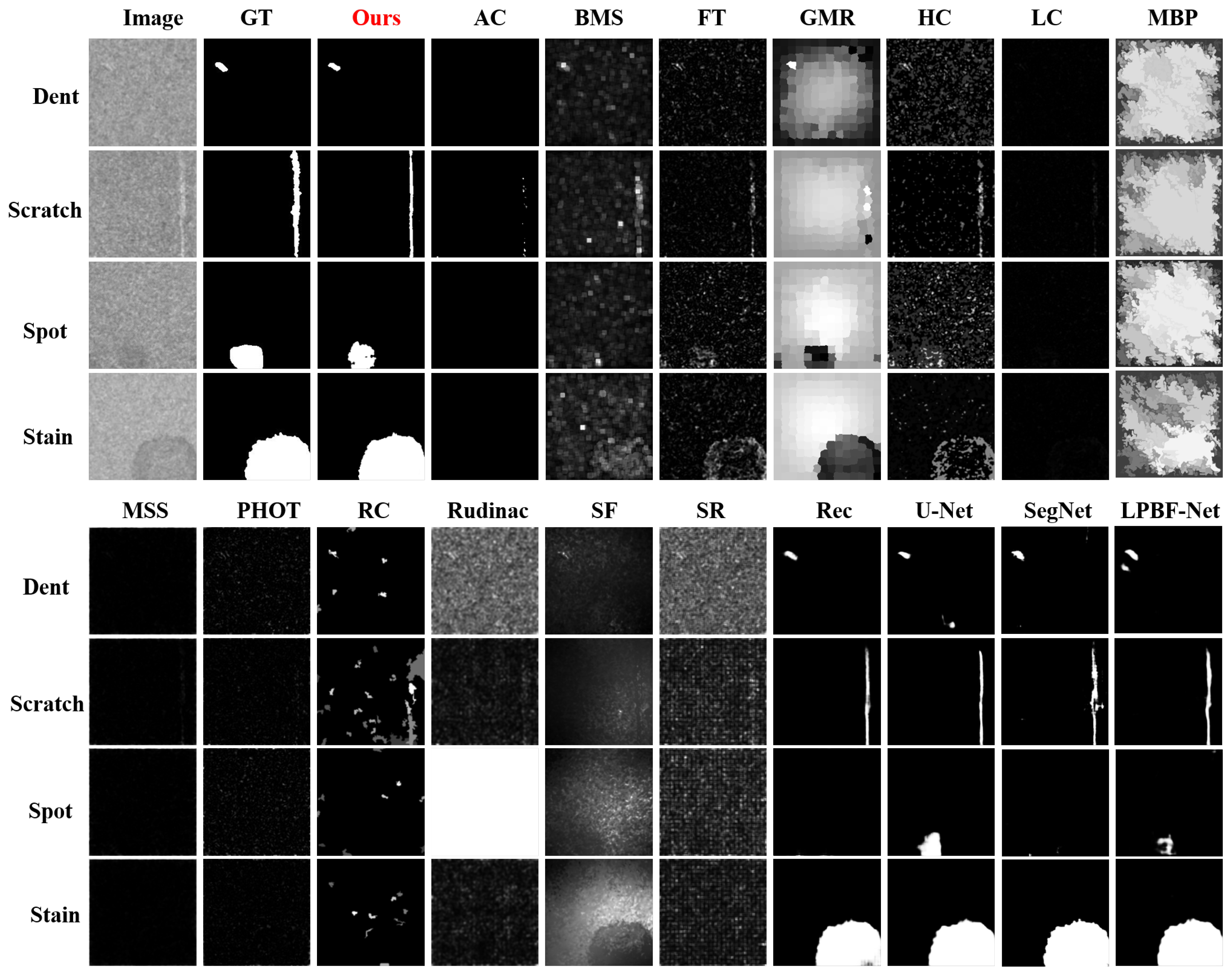
In addition to the quantitative comparison of F β , the MAE, and the Dice coefficient, visual results are also compared in this paper to make the experimental evaluation more comprehensive. The experimental results are shown in Figure 9, where the four defect types are compared. The first column of the upper half of the graph is the input image, the second is the annotated ground truth, the third is the results presented in this paper, and the remaining part shows the results of other methods. It can be seen that the detection results of many methods were pure black, such as those of AC, LC, MSS, and PHOT, which indicated that these methods failed to find defective areas. Other methods, such as BMS, FT, HC, and RC, found partial defect information, but they could not suppress non-defective areas. In addition, some methods, such as GMR, Rudinac, and SF, failed to correctly identify defective and non-defective areas, misidentifying non-defective areas as defective areas. The proposed USB-SG defect dataset had the characteristics of large differences in defect size. For example, the size of the dents was less than 0.5 mm, and the size of the stains was usually more than 5 mm. The traditional hand-crafted feature-extractor-based methods could not adapt to multi-scale features. In addition, there were difficulties such as weak defect features and unclear edges, which also affected the detection performance.
Compared to traditional methods, deep-learning-based approaches performed better. In the detection of dent-type defects, our model could completely detect the defective areas and suppress the non-defective areas. U-Net and LPBF-Net misidentified the features of the non-defective areas as defective. In the results for scratches, it could be seen that the integrity of the model proposed in this paper was better, while Rec, U-Net, and SegNet were worse. In the results for spots, it could be seen that Rec, SegNet, and LPBF-Net failed to identify defective areas, and the integrity of U-Net’s results was not as good as that of ours. In the detection results for stains, Rec could not find defective regions completely, and some defective areas were misjudged as non-defective regions. Based on the above comparison, it can be concluded that the proposed method had better detection results than those of other methods and could accurately distinguish defective from non-defective areas. However, the method proposed in this paper also has room for further improvement. For example, the completeness of the spot sample detection results was not satisfactory.
In order to test the computational efficiency of the model, the model was tested on a computer equipped with an NVIDIA 1080Ti GPU. By calculating the average value many times, it is found that the model could process more than 40 200 × 200 pixel images per second, thus achieving real-time speed. The processing speed of this model was much faster than that of manual inspection and has broad application prospects in the field of industrial surface defect inspection.

5. Conclusions

To improve the automation level of defect detection and promote the application of intelligent detection methods in product quality monitoring, in this paper, a defect inspection system was proposed to solve the problem of a defect inspection task for USB connectors. A defect dataset, USB-SG, which contained pixel-level defect locations, was collected and manually labeled. We proposed a defect inspection model that included three model optimization techniques. Firstly, a rich feature extraction block was designed to extract semantic and detailed information. Then, the feature fusion performance and the generalization ability of the model were improved through residual-based progressive integration. Finally, multi-step deep supervision was applied to improve the final prediction performance. The experimental results showed that the proposed model had better detection performance than that of other models; F β reached 0.7057, and the MAE was as low as 0.008. In addition, our model could achieve real-time processing speeds (>40 FPS ) on an NVIDIA 1080Ti GPU. Our proposed defect inspection system has a wide range of application prospects in industrial inspection tasks and can be used as a model for related researchers as technical support.
In the future, we plan to study further from two perspectives: First, considering that it takes many human resources to annotate the pixel-level ground truth, we plan to study a weakly supervised method to reduce the demand for manual annotations. Second, we intend to investigate more general inspection systems that can be adapted to defect inspection tasks for a variety of products.
Author Contributions

Conceptualization, G.F., W.L., Z.Z., J.L., Q.Z. and F.N.; methodology, G.F., W.L., Z.Z., J.L., Q.Z., F.N., H.C., F.S. and Y.S.; software, G.F.,W.L., Z.Z. and F.N.; validation, G.F., H.C., F.S. and Y.S.; formal analysis, G.F., J.L., Q.Z. and F.N.; investigation, G.F., W.L. and Z.Z.; resources, H.C., F.S. and Y.S.; data curation, G.F., W.L., Z.Z., and F.N.; writing—original draft preparation, W.L. and Z.Z.; writing—review and editing, J.L., Q.Z., and F.N.; visualization, H.C., F.S., Y.S., and G.F.; supervision, J.L. and Q.Z.; project administration, G.F. All authors have read and agreed to the published version of the manuscript.

Funding

This research was supported by the National Natural Science Foundation of China (No. 52105526, No. 51975394, No. 61903269, No. 51875380) and the China Postdoctoral Science Foundation (Nos. 2020M671383, 2020M681517).

Data Availability Statement

Not applicable.

Conflicts of Interest

On behalf of all authors, the corresponding author states that there are no conflicts of interest.

References

  1. Zhao, Y.J.; Yan, Y.H.; Song, K.C. Vision-based automatic detection of steel surface defects in the cold rolling process: Considering the influence of industrial liquids and surface textures. Int. J. Adv. Manuf. Technol. 2017, 90, 1665–1678. [Google Scholar] [CrossRef]
  2. Yang, L.; Huang, X.; Ren, Y.; Huang, Y. Steel Plate Surface Defect Detection Based on Dataset Enhancement and Lightweight Convolution Neural Network. Machines 2022, 10, 523. [Google Scholar] [CrossRef]
  3. Neogi, N.; Mohanta, D.K.; Dutta, P.K. Review of vision-based steel surface inspection systems. EURASIP J. Image Video Process. 2014, 2014, 50. [Google Scholar] [CrossRef] [Green Version]
  4. Ouyang, W.; Xu, B.; Hou, J.; Yuan, X. Fabric defect detection using activation layer embedded convolutional neural network. IEEE Access 2019, 7, 70130–70140. [Google Scholar] [CrossRef]
  5. Zhou, X.; Wang, Y.; Xiao, C.; Zhu, Q.; Lu, X.; Zhang, H.; Ge, J.; Zhao, H. Automated visual inspection of glass bottle bottom with saliency detection and template matching. IEEE Trans. Instrum. Meas. 2019, 68, 4253–4267. [Google Scholar] [CrossRef]
  6. Tsai, D.M.; Huang, Y.Q.; Chiu, W.Y. Deep learning from imbalanced data for automatic defect detection in multicrystalline solar wafer images. Meas. Sci. Technol. 2021, 32, 124003. [Google Scholar] [CrossRef]
  7. Song, K.; Yan, Y. A noise robust method based on completed local binary patterns for hot-rolled steel strip surface defects. Appl. Surf. Sci. 2013, 285, 858–864. [Google Scholar] [CrossRef]
  8. Mak, K.L.; Peng, P.; Yiu, K.F.C. Fabric defect detection using morphological filters. Image Vis. Comput. 2009, 27, 1585–1592. [Google Scholar] [CrossRef]
  9. Kang, X.; Zhang, E. A universal and adaptive fabric defect detection algorithm based on sparse dictionary learning. IEEE Access 2020, 8, 221808–221830. [Google Scholar] [CrossRef]
  10. Bissi, L.; Baruffa, G.; Placidi, P.; Ricci, E.; Scorzoni, A.; Valigi, P. Automated defect detection in uniform and structured fabrics using Gabor filters and PCA. J. Vis. Commun. Image Represent. 2013, 24, 838–845. [Google Scholar] [CrossRef]
  11. Fu, G.; Sun, P.; Zhu, W.; Yang, J.; Cao, Y.; Yang, M.Y.; Cao, Y. A deep-learning-based approach for fast and robust steel surface defects classification. Opt. Lasers Eng. 2019, 121, 397–405. [Google Scholar] [CrossRef]
  12. Silver, D.; Huang, A.; Maddison, C.J.; Guez, A.; Sifre, L.; Van Den Driessche, G.; Schrittwieser, J.; Antonoglou, I.; Panneershelvam, V.; Lanctot, M.; et al. Mastering the game of Go with deep neural networks and tree search. Nature 2016, 529, 484–489. [Google Scholar] [CrossRef] [PubMed]
  13. Krizhevsky, A.; Sutskever, I.; Hinton, G.E. ImageNet Classification with Deep Convolutional Neural Networks. In Proceedings of the International Conference on Neural Information Processing Systems, Lake Tahoe, NV, USA, 3–6 December 2012; pp. 1097–1105. [Google Scholar]
  14. Simonyan, K.; Zisserman, A. Very deep convolutional networks for large-scale image recognition. In Proceedings of the International Conference on Learning Representations, San Diego, CA, USA, 7–9 May 2015; pp. 1–14. [Google Scholar]
  15. Kim, Y.; Kim, D. A CNN-based 3D human pose estimation based on projection of depth and ridge data. Pattern Recognit. 2020, 106, 107462. [Google Scholar] [CrossRef]
  16. Tian, C.; Xu, Y.; Zuo, W.; Zhang, B.; Fei, L.; Lin, C.W. Coarse-to-fine CNN for image super-resolution. IEEE Trans. Multimed. 2020, 23, 1489–1502. [Google Scholar] [CrossRef]
  17. Gao, H.; Cheng, B.; Wang, J.; Li, K.; Zhao, J.; Li, D. Object classification using CNN-based fusion of vision and LIDAR in autonomous vehicle environment. IEEE Trans. Ind. Inform. 2018, 14, 4224–4231. [Google Scholar] [CrossRef]
  18. Li, Y.; Li, G.; Jiang, M. An End-to-End Steel Strip Surface Defects Recognition System Based on Convolutional Neural Networks. Steel Res. Int. 2016, 88, 1600068. [Google Scholar]
  19. Benbarrad, T.; Eloutouate, L.; Arioua, M.; Elouaai, F.; Laanaoui, M.D. Impact of Image Compression on the Performance of Steel Surface Defect Classification with a CNN. J. Sens. Actuator Netw. 2021, 10, 73. [Google Scholar] [CrossRef]
  20. Imoto, K.; Nakai, T.; Ike, T.; Haruki, K.; Sato, Y. A CNN-based transfer learning method for defect classification in semiconductor manufacturing. In Proceedings of the 2018 International Symposium on Semiconductor Manufacturing (ISSM), Tokyo, Japan, 10–11 December 2018; pp. 1–3. [Google Scholar]
  21. Ren, R.; Hung, T.; Tan, K.C. A generic deep-learning-based approach for automated surface inspection. IEEE Trans. Cybern. 2018, 48, 929–940. [Google Scholar] [CrossRef]
  22. Wang, T.; Chen, Y.; Qiao, M.; Snoussi, H. A fast and robust convolutional neural network-based defect detection model in product quality control. Int. J. Adv. Manuf. Technol. 2018, 94, 3465–3471. [Google Scholar] [CrossRef]
  23. Zhang, M.; Wu, J.; Lin, H.; Yuan, P.; Song, Y. The application of one-class classifier based on CNN in image defect detection. Procedia Comput. Sci. 2017, 114, 341–348. [Google Scholar] [CrossRef]
  24. Huang, Y.; Qiu, C.; Wang, X.; Wang, S.; Yuan, K. A compact convolutional neural network for surface defect inspection. Sensors 2020, 20, 1974. [Google Scholar] [CrossRef] [PubMed]
  25. Tabernik, D.; Šela, S.; Skvarč, J.; Skočaj, D. Segmentation-based deep-learning approach for surface-defect detection. J. Intell. Manuf. 2020, 31, 759–776. [Google Scholar] [CrossRef] [Green Version]
  26. Itti, L.; Koch, C.; Niebur, E. A model of saliency-based visual attention for rapid scene analysis. IEEE Trans. Pattern Anal. Mach. Intell. 1998, 20, 1254–1259. [Google Scholar] [CrossRef] [Green Version]
  27. Achanta, R.; Estrada, F.; Wils, P.; Süsstrunk, S. Salient region detection and segmentation. In Proceedings of the International Conference on Computer Vision Systems, Santorini, Greece, 12–15 May 2008; pp. 66–75. [Google Scholar]
  28. Zhang, J.; Sclaroff, S. Saliency detection: A boolean map approach. In Proceedings of the IEEE International Conference on Computer Vision, Sydney, Australia, 1–8 December 2013; pp. 153–160. [Google Scholar]
  29. Cheng, M.M.; Mitra, N.J.; Huang, X.; Torr, P.H.; Hu, S.M. Global contrast based salient region detection. IEEE Trans. Pattern Anal. Mach. Intell. 2014, 37, 569–582. [Google Scholar] [CrossRef] [Green Version]
  30. Perazzi, F.; Krähenbühl, P.; Pritch, Y.; Hornung, A. Saliency filters: Contrast based filtering for salient region detection. In Proceedings of the 2012 IEEE Conference on Computer Vision and Pattern Recognition, Providence, RI, USA, 16–21 June 2012; pp. 733–740. [Google Scholar]
  31. Huang, Y.; Qiu, C.; Yuan, K. Surface defect saliency of magnetic tile. Vis. Comput. 2020, 36, 85–96. [Google Scholar] [CrossRef]
  32. Ronneberger, O.; Fischer, P.; Brox, T. U-net: Convolutional networks for biomedical image segmentation. In Proceedings of the International Conference on Medical Image Computing and Computer-Assisted Intervention, Munich, Germany, 5–9 October 2015; pp. 234–241. [Google Scholar]
  33. Feng, C.; Liu, M.Y.; Kao, C.C.; Lee, T.Y. Deep active learning for civil infrastructure defect detection and classification. Comput. Civ. Eng. 2017, 2017, 298–306. [Google Scholar]
  34. Yang, G.; Liu, K.; Zhao, Z.; Zhang, J.; Chen, X.; Chen, B.M. Datasets and methods for boosting infrastructure inspection: A survey on defect classification. In Proceedings of the 2022 IEEE 17th International Conference on Control & Automation (ICCA), Naples, Italy, 27–30 June 2022; pp. 15–22. [Google Scholar]
  35. Iandola, F.N.; Han, S.; Moskewicz, M.W.; Ashraf, K.; Dally, W.J.; Keutzer, K. SqueezeNet: AlexNet-level accuracy with 50x fewer parameters and <0.5MB model size. arXiv 2016, arXiv:1602.07360. [Google Scholar]
  36. Hou, Q.; Cheng, M.M.; Hu, X.; Borji, A.; Tu, Z.; Torr, P.H. Deeply supervised salient object detection with short connections. In Proceedings of the IEEE Conference on Computer Vision and Pattern Recognition, Honolulu, HI, USA, 21–26 July 2017; pp. 3203–3212. [Google Scholar]
  37. Zhang, P.; Wang, D.; Lu, H.; Wang, H.; Ruan, X. Amulet: Aggregating multi-level convolutional features for salient object detection. In Proceedings of the IEEE International Conference on Computer Vision, Venice, Italy, 22–29 October 2017; pp. 202–211. [Google Scholar]
  38. He, K.; Zhang, X.; Ren, S.; Sun, J. Deep residual learning for image recognition. In Proceedings of the IEEE Conference on Computer Vision and Pattern Recognition, Las Vegas, NV, USA, 27–30 June 2016; pp. 770–778. [Google Scholar]
  39. Jia, Y.; Shelhamer, E.; Donahue, J.; Karayev, S.; Long, J.; Girshick, R.; Guadarrama, S.; Darrell, T. Caffe: Convolutional architecture for fast feature embedding. In Proceedings of the 22nd ACM International Conference on Multimedia, Orlando, FL, USA, 3–7 November 2014; pp. 675–678. [Google Scholar]
  40. Sørensen, T.J. A Method of Establishing Groups of Equal Amplitude in Plant Sociology Based on Similarity of Species Content and Its Application to Analyses of the Vegetation on Danish Commons; Munksgaard: København, Denmark, 1948. [Google Scholar]
  41. Li, X.; Sun, X.; Meng, Y.; Liang, J.; Wu, F.; Li, J. Dice loss for data-imbalanced NLP tasks. arXiv 2019, arXiv:1911.02855. [Google Scholar]
  42. Lin, T.Y.; Goyal, P.; Girshick, R.; He, K.; Dollár, P. Focal loss for dense object detection. In Proceedings of the IEEE International Conference on Computer Vision, Venice, Italy, 22–29 October 2017; pp. 2980–2988. [Google Scholar]
  43. Achanta, R.; Hemami, S.; Estrada, F.; Susstrunk, S. Frequency-tuned salient region detection. In Proceedings of the 2009 IEEE Conference on Computer Vision and Pattern Recognition, Miami, FL, USA, 20–25 June 2009; pp. 1597–1604. [Google Scholar]
  44. Yang, C.; Zhang, L.; Lu, H.; Ruan, X.; Yang, M.H. Saliency detection via graph-based manifold ranking. In Proceedings of the IEEE Conference on Computer Vision and Pattern Recognition, Portland, OR, USA, 23–28 June 2013; pp. 3166–3173. [Google Scholar]
  45. Zhai, Y.; Shah, M. Visual attention detection in video sequences using spatiotemporal cues. In Proceedings of the 14th ACM International Conference on Multimedia, Santa Barbara, CA, USA, 23–27 October 2006; pp. 815–824. [Google Scholar]
  46. Zhang, J.; Sclaroff, S.; Lin, Z.; Shen, X.; Price, B.; Mech, R. Minimum barrier salient object detection at 80 fps. In Proceedings of the IEEE International Conference on Computer Vision, Santiago, Chile, 7–13 December 2015; pp. 1404–1412. [Google Scholar]
  47. Achanta, R.; Süsstrunk, S. Saliency detection using maximum symmetric surround. In Proceedings of the 2010 IEEE International Conference on Image Processing, Hong Kong, China, 26–29 September 2010; pp. 2653–2656. [Google Scholar]
  48. Aiger, D.; Talbot, H. The phase only transform for unsupervised surface defect detection. In Proceedings of the 2010 IEEE Computer Society Conference on Computer Vision and Pattern Recognition, Hong Kong, China, 26–29 September 2010; pp. 295–302. [Google Scholar]
  49. Rudinac, M.; Jonker, P.P. Saliency detection and object localization in indoor environments. In Proceedings of the 2010 20th International Conference on Pattern Recognition, Istanbul, Turkey, 23–26 August 2010; pp. 404–407. [Google Scholar]
  50. Hou, X.; Zhang, L. Saliency detection: A spectral residual approach. In Proceedings of the 2007 IEEE Conference on Computer Vision and Pattern Recognition, Minneapolis, MN, USA, 17–22 June 2007; pp. 1–8. [Google Scholar]
  51. Cao, Y.; Fu, G.; Yang, J.; Cao, Y.; Yang, M.Y. Accurate salient object detection via dense recurrent connections and residual-based hierarchical feature integration. Signal Process. Image Commun. 2019, 78, 103–112. [Google Scholar] [CrossRef]
  52. He, M.; Zhao, Q.; Gao, H.; Zhang, X.; Zhao, Q. Image Segmentation of a Sewer Based on Deep Learning. Sustainability 2022, 14, 6634. [Google Scholar] [CrossRef]
  53. Nemati, S.; Ghadimi, H.; Li, X.; Butler, L.G.; Wen, H.; Guo, S. Automated Defect Analysis of Additively Fabricated Metallic Parts Using Deep Convolutional Neural Networks. J. Manuf. Mater. Process. 2022, 6, 141. [Google Scholar] [CrossRef]
Figure 1. The defect inspection system and dataset generation process.
Machines 11 00124 g001
Figure 2. The sample images and ground truth of the five types of defects.
Machines 11 00124 g002
Figure 3. The architecture of the modelling approach via rich feature extraction and residual-based progressive integration.
Machines 11 00124 g003
Figure 4. Comparison of the proposed feature extraction strategy and the two existing structures. (a) Extraction of features by using the last layer in the deep stage [24,25]. (b) Extraction of features by using the last layer in all stages [36,37]. (c) Proposed: Extraction of features by using all of the layers in all stages.
Machines 11 00124 g004
Figure 5. The details of the generative process of the ith rich feature extraction block.
Machines 11 00124 g005
Figure 6. A detailed structural diagram of the residual-based progressive integration scheme.
Machines 11 00124 g006
Figure 7. A diagram of the predicted results and ground truth.
Machines 11 00124 g007
Figure 8. Visual comparisons of different predictions. Four types of defects (dents, scratches, spots, and stains) are shown in order.
Machines 11 00124 g008
Figure 9. Visual comparisons of different defect/object localization models.
Machines 11 00124 g009
Table 1. The numbers of samples in the training and test sets for the different types of defects in the USB-SG dataset.
Defect TypeTotalTraining SetTesting Set
Dent1169323
Scratch1209624
Spot685513
Stain564511
Normal32325964
Total683548135
Table 2. A comparative evaluation of different feature extraction strategies. SQ-a: Extraction of features by using the last layer in the deep stage [24,25]. SQ-b: Extraction of features by using the last layer in all stages [36,37]. Proposed SQ-RFE: Extraction of features by using all of the layers in all stages. The precision, recall, F β , MAE-1, and Dice coefficient were calculated by using the dent, scratch, spot, and stain test set. The MAE-2 was calculated by using all of the defect types in the test set.
ModelPrecisionRecall F β MAE-1MAE-2Dice
SQ-a0.59540.71400.59580.01850.00980.5587
SQ-b0.65720.67880.63400.01740.00940.6057
SQ-RFE0.68880.70610.67020.01670.00880.6515
Table 3. The comparative evaluation of the proposed model with/without the use of RPI.
ModelPrecisionRecall F β MAE-1MAE-2Dice
SQ-Unet0.65720.67880.63400.01740.00940.6057
SQ-RPI0.69880.70690.67810.01700.00900.6515
SQ-RFE0.68880.70610.67020.01670.00880.6484
SQ-RFE-RPI0.70260.70420.68620.01580.00840.6640
Table 4. The comparative evaluation of the proposed SQ-RFE-RPI and SQ-RFE-RPI-MsDS models when using different total amounts of supervision. Note that only the predictions with the best performance for each model are recorded in the table. The best results of for F β , the MAE, and the Dice coefficient are shown in bold.
ModelPrecisionRecall F β MAE-1MAE-2Dice
SQ-RFE-RPI0.70260.70420.68620.01580.00840.6640
SQ-RFE-RPI-MsDS, M = 4 0.71740.71670.69830.01620.00860.6821
SQ-RFE-RPI-MsDS, M = 5 0.74130.69950.70570.01510.00800.6854
SQ-RFE-RPI-MsDS, M = 6 0.71680.70940.69880.01600.00850.6823
SQ-RFE-RPI-MsDS, M = 7 0.71310.71050.69180.01620.00860.6734
SQ-RFE-RPI-MsDS, M = 8 0.71890.71340.69210.01590.00840.6783
SQ-RFE-RPI-MsDS, M = 9 0.71140.71160.68110.01650.00870.6745
Table 5. The comparative evaluation of the proposed SQ-RFE-RPI-MsDS ( M = 5 ) model in different predictions.
PredictionPrecisionRecall F β MAE-1MAE-2Dice
P 1 0.74130.69950.70570.0151130.007990.6854
P 2 0.74480.70390.70540.0151350.008000.6801
P 3 0.74420.69990.70360.0151810.008030.6787
P 4 0.73540.69810.70040.0153060.008090.6768
P 5 0.72750.68230.69240.0156340.008260.6484
Table 6. The comparative evaluation of the proposed SQ-RFE-RPI-MsDS model with different loss functions.
Loss FunctionPrecisionRecall F β MAE-1MAE-2Dice
Cross-entropy0.74130.69950.70570.01510.00800.6854
Dice loss0.71250.72170.69730.01600.00850.6812
Focal loss ( a = 1 , γ = 0.5 )0.74780.73520.70880.01490.00780.6921
Focal loss ( a = 1 , γ = 2 )0.71410.73080.70020.01530.00840.6765
Table 7. The comparative evaluation of different defect/object localization models on the USB-SG defect dataset. The best results for F β , the MAE, and the Dice coefficient are shown in bold. It should be noted that higher values of F β and lower values of the MAE indicate better performance.
ModelPrecisionRecall F β MAE-1MAE-2Dice
AC [27]0.53280.40650.22490.05050.02680.1249
BMS [28]0.22830.63100.21810.12020.13030.3583
FT [43]0.16870.64280.16860.07020.06210.2091
GMR [44]0.19140.27830.12590.50190.51690.2060
HC [29]0.18800.65990.18210.08840.08620.3204
LC [45]0.15790.63330.15860.05390.03060.0048
MBP [46]0.14000.44900.12500.64970.71750.0979
MSS [47]0.07700.24450.07150.06400.04070.0060
PHOT [48]0.07660.43740.07670.06940.04810.0383
RC [29]0.18130.58840.19060.06110.04230.3533
Rudinac [49]0.14750.25530.10840.24580.21210.0637
SF [30]0.19240.46720.17520.20900.19670.0724
SR [50]0.12200.18980.08750.21800.20580.0720
U-Net [32]0.62630.78050.63880.01830.00980.6217
Rec [51]0.67820.82790.68830.01620.00850.6789
SegNet [52]0.67790.82770.68620.01600.00840.6797
LPBF-Net [53]0.67930.81590.69680.01570.00820.6806
Proposed0.74130.69950.70570.01510.00800.6854
Disclaimer/Publisher’s Note: The statements, opinions and data contained in all publications are solely those of the individual author(s) and contributor(s) and not of MDPI and/or the editor(s). MDPI and/or the editor(s) disclaim responsibility for any injury to people or property resulting from any ideas, methods, instructions or products referred to in the content.