Early Fault Diagnosis of Rolling Bearing Based on Threshold Acquisition U-Net

Abstract

Considering the problem that the early fault signal of rolling bearing is easily interfered with by background information, such as noise, and it is difficult to extract fault features, a method of rolling bearing early fault diagnosis based on the threshold acquisition U-Net (TA-UNet) is proposed. First, to improve the feature extraction ability of U-Net, the channel spatial threshold acquisition network (CS-TAN) and the dilated convolution module (DCM) based on different dilated rate combinations are introduced into the U-Net to construct the TA-UNet. Among them, the CS-TAN can adaptively learn the threshold, reduce the interference of noise in the signal, and the DCM can improve the multi-scale feature extraction ability of the network. Then, the TA-UNet is used for early fault diagnosis, and the method is divided into two steps: The model training phase and the vibration signal fault feature extraction phase. In the first step, additive gaussian white noise is added to the vibration signal to obtain the noise-added vibration signal, and the TA-UNet is trained to learn how to denoise the noise-added vibration signal. In the second step, the trained TA-UNet is used to extract the fault features of vibration signals and diagnose the early fault types of rolling bearing. The two-step method solves the problem that U-Net, as a supervised neural network, needs corresponding labeled data to be trained, as it realizes the fault diagnosis of unlabeled data. The feature extraction capability of the TA-UNet is evaluated by denoising the simulated signal of rolling bearing. The effectiveness of the proposed diagnostic method is demonstrated by the early fault diagnosis of open-source datasets.

1. Introduction

Vibration monitoring is one of the most effective tools for the fault diagnosis of rolling bearings [1,2,3]. When a local fault occurs, the bearing can generate different characteristic frequencies depending on which surface the fault affects, and people diagnose the fault by analyzing the vibration signal [4,5]. Wear is the inevitable progressive material loss of a part and is one of the most common forms of failure of parts (e.g., bearing, gear) [6]. For example, foreign matter entering the bearing causes excessive grinding damage, pockmarks, and abrasions or grooves on the rolling elements and raceway, etc. [7], and the failure gradually becomes serious over time, eventually leading to more serious consequences. However, the fault feature is very weak in the initial stage of the bearing wear [8], and with the interference of the surrounding environment (collectively referred to as noise in this paper), the vibration signal becomes complex, resulting in a decrease in the accuracy of diagnosis [9]. Therefore, it is imperative to effectively extract the fault characteristic of rolling bearing vibration signals under noise background.

In recent years, scholars have proposed many signal processing methods and applied them to the vibration signal fault feature extraction of rolling bearing. Yu et al. [10] used empirical mode decomposition (EMD) and the Hilbert spectrum for bearing fault diagnosis. Guo et al. [11] proposed a multi-stage reduction method based on ensemble empirical mode decomposition (EEMD), wavelet denoising, and modulation signal bispectrum (MSB) to extract fault characteristics and diagnose early bearing faults. Liu et al. [12] proposed an Integral Extension LMD (IELMD) method and used it in wind turbine denoising and fault diagnosis. Gu et al. [13] proposed an adaptive stochastic resonance denoising method based on variational mode decomposition (VMD) and quantum particle swarm optimization. Ni et al. [14] proposed a fault information-guided VMD method (FIVMD), which solves the limitations of the VMD method in selecting the mode number and bandwidth control parameters, and avoids parts interfering with bearing signal. Pang et al. [15] proposed a recursive variational mode extraction (RVME) signal decomposition algorithm based on VME. This method can adaptively determine the initial center frequency and penalty factor of specific stator component reconstruction to adaptively decompose the signal and extract weak fault features in the signal. Lu et al. [16] also proposed a new dynamic modeling method: the graphical modeling wavelet packet coefficient (GMWPC) realized the fault warning and identification of rolling bearings.

Deep learning (DL) has recently been widely developed and successfully applied to various signal-processing tasks [17,18,19]. The fundamental purpose of the DL is to map the original data to the feature space by learning a nonlinear input function under the multi-layer neural network structure to extract the original data’s implicit features [20]. Convolution neural network (CNN), a deep neural network among many deep neural networks, is very popular because of its sparse connection and weight-sharing feature [21]. Notably, CNNs [22,23] have brought many significant breakthroughs in image recognition. Inspired by CNNs in image recognition, Ronneberge et al. [24] proposed a fully convolutional neural network, U-Net, with an encoder–decoder architecture for medical image segmentation. U-Net is widely used in various image processing tasks due to its small training set and high segmentation accuracy. For example, Cai et al. [25] proposed Dense-UNet, which integrates dense connections based on U-Net to deepen the depth of the network architecture and achieve feature reuse to segment the multiphoton microscopy (MPM) images of skin cells more accurately. Furthermore, Feng et al. [26] proposed a pixel-level segmentation framework for fatigue steel crack detection accuracy by improving U-Net.

U-Net has achieved great success in image processing and its application has been promoted in other fields. Of these, Qiu et al. [27] proposed an ECG signal noise reduction system. First, the improved U-Net is used for denoising, and DR-net is used for detail recovery. Stoller et al. [28] also proposed a Wave-U-Net that can be directly used for time-domain signals, which avoids the error caused by converting time-domain signals into the frequency domain for audio source separation. Additionally, Hao et al. [29] combined dilated convolution and conditional generative adversarial networks (CGAN) to improve the effect of speech enhancement under low signal-to-noise ratio (SNR) conditions (up to −20 dB). In this paper, U-Net is used for the fault feature extraction of rolling bearing vibration signals, and the following problems are encountered:

• U-Net has a weak ability to extract fault features of vibration signals under low SNR conditions.
• U-Net is a kind of deep supervised learning network that needs corresponding label data to be trained [30]. This is a difficult task under actual conditions since labeling the condition monitoring data of rolling bearings would take more human and material resources than just recording them [31].

To solve the above problems, an improved U-Net, namely, the threshold acquisition U-Net (TA-UNet), is proposed, which is used for the early fault diagnosis of rolling bearing.

First, the channel spatial threshold acquisition network (CS-TAN) obtains the threshold by extracting the channel and spatial information of the feature map. The dilated convolution module (DCM) uses a combination of dilated convolution with different expansion rate to obtain a multi-scale feature extraction capability. Then, the CS-TAN and the DCM are introduced into the U-Net to construct the TA-UNet, which has a robust feature extraction ability.

Finally, the TA-UNet is used for bearing early fault diagnosis. U-Net, as a deeply supervised network, needs corresponding labels to be trained. In this paper, Transfer Learning (TL) is used to solve this problem. TL focuses on using the knowledge gained from a problem to solve a different but related problem. TL has been applied to the research of fault diagnosis. Wen et al. [32] proposed a deep transfer learning method for fault diagnosis based on sparse autoencoder that can learn common features across different working conditions. Wang et al. [33] developed a multi-scale deep intra-class transfer learning model with conditional maximum mean discrepancy (MMD), and applied it to bearing fault diagnosis. Zhang et al. [34] proposed a supervised contrastive learning-based domain adaptation network (SCLDAN) for the cross-domain fault diagnosis of the rolling bearing. Therefore, using the TA-UNet’s super feature extraction ability and TL, a two-stage rolling bearing fault diagnosis method is proposed. In the first stage, the TA-UNet is trained with the noise-added vibration signal, and in the second stage the fault characteristics of the vibration signal are extracted with the trained TA-UNet and the fault type is diagnosed by envelope spectrum analysis.

The remainder of this paper is organized as follows. In Section 2, the TA-UNet, which integrates CS-TAN and DCM into U-Net, and a two-stage fault diagnosis method of rolling bearing based on the TA-UNet are proposed. In Section 3, the TA-UNet proposed in Section 2 is used to de-noise the simulation signals with different SNR and compare them with different models to prove their feature extraction capability. In Section 4, the fault diagnosis method proposed in Section 2 is used to diagnose the two sets of open-source datasets early and compare the RMS method to prove the superiority of the proposed fault diagnosis method. Conclusions are drawn in Section 5.

2. Methodology

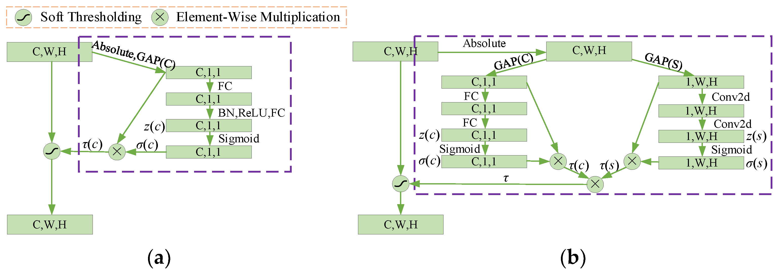
2.1. Channel Spatial Threshold Acquisition Network

Zhao et al. [35] proposed DRSN to solve the problem that noise in vibration signals affects fault diagnosis accuracy. To a certain extent, the working principle of DRSN can be understood as follows: the network adaptively acquires a set of soft thresholds [36] to reduce noise interference in the signal when the network extracts signal features. The function of soft threshold, as shown in Equation (1).

$$y=\left\{\begin{array}{llll}x-\tau & & & x>\tau \\ 0& & & -\tau \le x\le \tau \\ x+\tau & & & x<-\tau \end{array}\right.$$

(1)

where x is the input feature, y is the output feature, and τ is the threshold.

Figure 1 shows the structure of the channel threshold acquisition network (C-TAN) and channel spatial threshold acquisition network (CS-TAN). The C-TAN is shown in Figure 1a. The global average pooling (GAP) is applied to the absolute value of the feature map X to get a 1-D vector containing the channel information of the feature map X. The 1-D vector is passed into a two-layer full connection (FC) network to obtain the channel scale parameter, and it is scaled to the range (0, 1) through the sigmoid function, as shown in Equation (2).

$$\sigma \left(c\right)=\frac{1}{1+e^{-z\left(c\right)}}$$

(2)

where z(c) is the channel scale parameter, σ(c) is the corresponding scaling parameter, and c is the channel information of the feature map X.

Finally, σ(c) and 1-D vector are multiplied to get the thresholding containing the channel information of the feature map X, as shown in Equation (3).

$$\tau \left(c\right)=\sigma \left(c\right)·G_c\left|X\right|$$

(3)

where $G_c\left|X\right|$ is the 1-D vector, τ(c) is the channel threshold of feature map X.

The CS-TAN is shown in Figure 1b. Based on C-TAN, a branch of spatial thresholding is added to the network, and the threshold acquisition by the network contains the channel and spatial information of feature map X so that the accuracy of threshold acquisition is improved. Specifically, on the spatial thresholding acquisition branch, the GAP is applied to the absolute values of the feature map X to get a 2-D vector containing the spatial information of the feature map X. The 2-D vector is passed into a two-layer Conv2d network to obtain the spatial scale parameter, and it is also scaled to the range (0, 1) through the sigmoid function, as shown in Equation (4).

$$\sigma \left(s\right)=\frac{1}{1+e^{-z\left(s\right)}}$$

(4)

where z(s) is the spatial scale parameter, σ(s) is the corresponding scaling parameter, and s is the spatial information of the feature map X.

Later, σ(s) and 2-D vector are multiplied to get the thresholding containing the spatial information of the feature map X, as shown in Equation (5).

$$\tau \left(s\right)=\sigma \left(s\right)\cdot G_s\left|X\right|$$

(5)

where $G_s\left|X\right|$ is the 2-D vector, τ(s) is the spatial threshold of the feature map X.

Finally, τ(c) and τ(s) are multiplied to obtain the thresholding τ containing the channel and spatial information of the feature map X, as shown in Equation (6).

$$\tau =\tau \left(c\right)\cdot \tau \left(s\right)$$

(6)

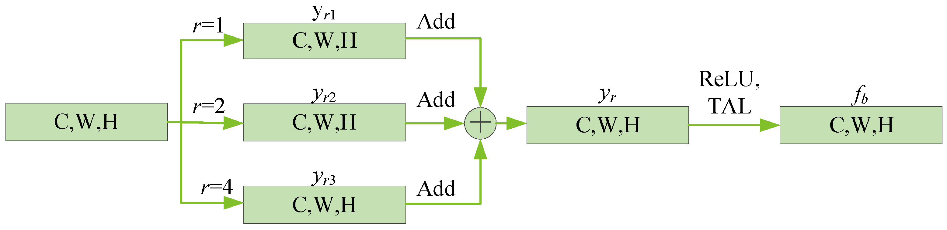
2.2. Dilated Convolution Module

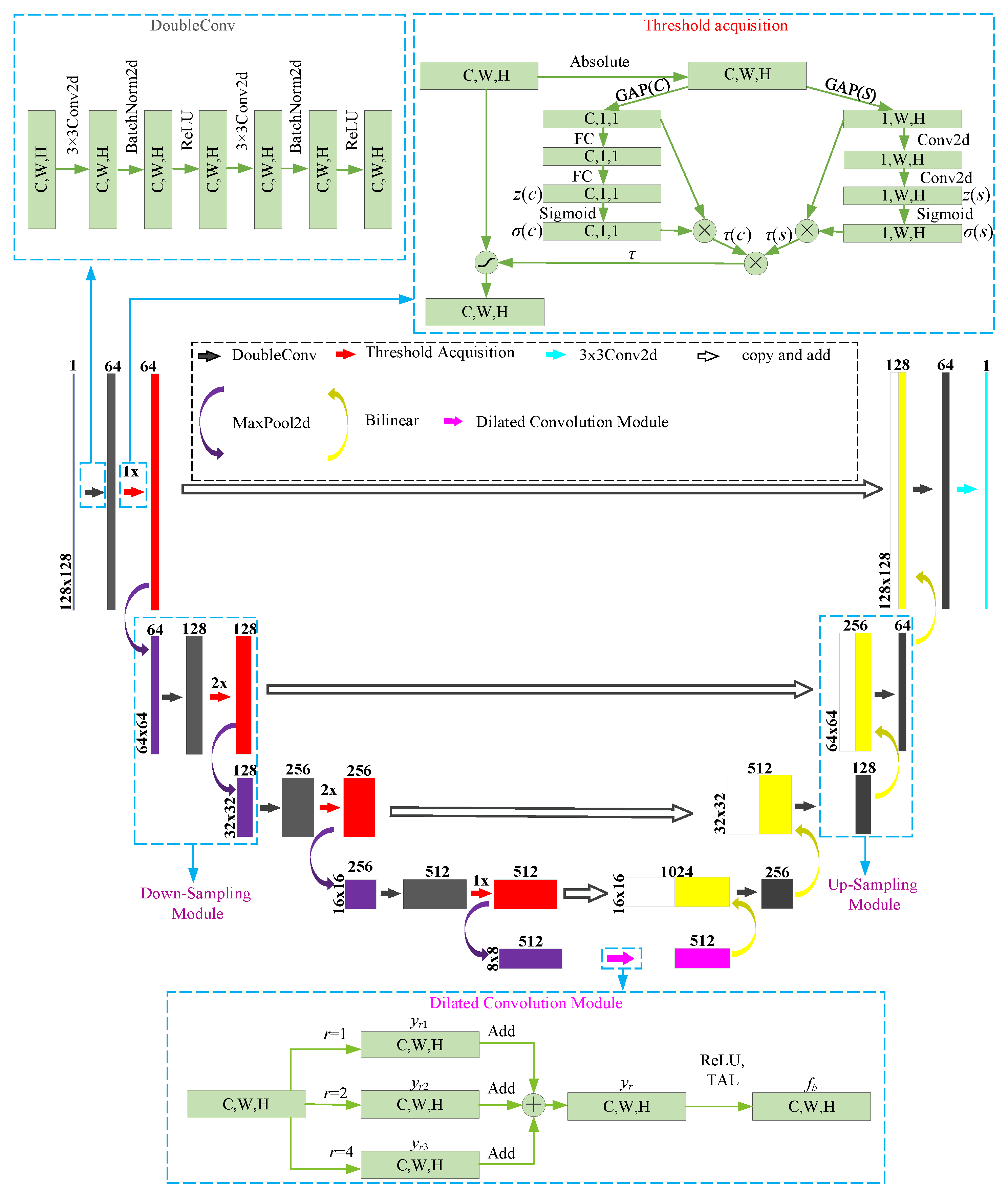
The receptive fields of the convolutional networks refer to the area size that can be mapped on the original data by the pixel points on the output feature map [37]. The larger the receptive field is, the more extensive the range of the original feature map it learns is. Notably, it may contain more comprehensive information and higher-level features in the feature map. The dilated convolution is to inject holes (points with a value of 0) into ordinary convolution to expand the convolution kernel. Thus, the size of receptive fields is enlarged [38].

For a 2-D input $x\left[i,j\right]$, the output $\mathrm{y}\left[i,j\right]$ of convolution on it with a filter $\omega \left[m,n\right]$ of size $\left[m,n\right]$ is shown in Equation (7).

$$\mathrm{y}\left[i,j\right]=\left(x\ast \omega \right)\left(i,j\right)={\displaystyle \sum _{m,n}x\left[i+m,j+n\right]\omega \left[m,n\right]}$$

(7)

Compared with the ordinary convolution, the dilated rate r is added to the dilated convolution. The output of a dilated convolution is expressed by Equation (8).

$${\mathrm{y}}_r\left[i,j\right]={\displaystyle \sum _{m,n}x\left[i+r\cdot m,j+r\cdot n\right]\omega \left[m,n\right]}$$

(8)

The receptive field calculation of 2-D dilated convolution is shown in Equation (9).

$$F_{i+1}=\left(2^{i+2}-1\right)\times \left(2^{i+2}-1\right)$$

(9)

where $F_{i+1}$ is the receptive fields of the 2-D dilated convolution, and i + 1 is the dilated rate.

Figure 2 shows the dilated convolution module (DCM) with exponentially increasing dilated rate (r = 1, 2, 4), stride = 1, kernel size = 3. As shown in Figure 2, the DCM’s dilated convolution layer adopts branches to obtain information on different scales and improve the network’s computing efficiency [39]. Subsequently, input the same data for different dilated convolution branches and add them together. Then, output the result of the DCM after the outcome of dilated convolution layer is fused by the ReLU layer and thresholding acquisition layer (TAL).

The dilated convolution output of the dilated rate (r = 1, 2, 4) in the DCM is recorded as y_r1, y_r2, y_r3, then the output y_r of dilated convolution layer is shown in Equation (10).

$$y_r=y_{r1}+y_{r2}+y_{r3}$$

(10)

If the threshold obtained is τ_b, the output f_b of the DCM is shown in Equation (11).

$$f_b=\left\{\begin{array}{lll}\max \left({0,\mathrm{y}}_r\right)-{\tau }_b& & x>{\tau }_b\\ 0& & -{\tau }_b\le x\le {\tau }_b\\ \max \left({0,\mathrm{y}}_r\right)+{\tau }_b& & x<-{\tau }_b\end{array}\right.$$

(11)

where max (0, y_r) is the output of the ReLU layer.

2.3. TA-UNet

Figure 3 shows the structure of TA-UNet. As shown, the TA-UNet is improved based on U-Net, mainly composed of four parts: encoder, decoder, DCM, and copy and add. The encoder and decoder are composed of four down-sampling modules and four up-sampling modules in cascade. The DCM is consistent with that proposed in Section 2.2. The principle of U-Net for signal noise reduction is that the hidden features of the signal are extracted by down-sampling the signal, and then the signal is reconstructed by up-sampling to achieve noise reduction. The differences between TA-UNet and U-Net: (1) the CS-TAN is added to the down-sampling module to reduce the signal’s noise interference when extracting the signal’s implicit feature; (2) the DCM is added at the bottleneck to improve the multi-scale feature extraction ability of the network; (3) up-sampling changes from transposed convolution to bilinear interpolation combined with Conv2d, avoiding checkerboard pattern [40].

2.3.1. Down-Sampling Module

When the down-sampling module is working, the channels of the feature map are doubled through a DoubleConv (DoC) layer (including two 3 × 3 Conv2d, one Batchnorm2d, and two ReLU). Then, j threshold acquisition (TA) layers are used to reduce the interference of noise in the feature map, and finally, the down-sampling (Maxpool, Mp) layer is used to halve the size of the feature map. Each pass through a down-sampling module, the size of the feature map is halved, and the number of channels is doubled. If the input of the ith down-sampling module of TA-UNet is $x_d^i$, the corresponding output $y_d^i$ is shown in Equation (12).

$$y_d^i=F_D^i\left(x_d^i\right)=F_{MP}^i\left(F_{{}_{TA}}^{i,j}\left(F_{{}_{DoC}}^i\left(x_d^i\right)\right)\right)$$

(12)

where $F_D^i\left(·\right)$ is the mapping of the down-sampling module, $F_{MP}^i\left(·\right)$ is the feature mapping of the Mp layer, $F_{{}_{TA}}^{i,j}\left(·\right)$ is the feature mapping of the TA layer, and $F_{{}_{DoC}}^i\left(·\right)$ is the feature mapping of the DoC layer.

2.3.2. Up-Sampling Module

When the up-sampling module is working, the size of the feature map is doubled through an up-sampling (bilinear interpolation, BI) layer. Considering that the details of the shallow network are well preserved, the down-sampling feature map with the same resolution corresponding to the copy and add fusion is used. Finally, the channel is halved through the DoC layer. Each pass through an up-sampling module, the size of the feature map is doubled, and the number of channels is halved. If the input of the kth up-sampling module of TA-UNet is $x_u^k$, the output of the up-sampling module shown in Equation (13).

$$y_u^k=F_U^k\left(x_u^k\right)=F_{{}_{DoC}}^k\left(CA{T}^k\left(F_{{}_{TA}}^{5-k,j}\left(x_{{}_d}^{5-k}\right),F_{BL}^k\left(x_u^k\right)\right)\right)$$

(13)

where $F_U^k\left(·\right)$ is the mapping of the up-sampling module, $CA{T}^k\left(·\right)$ is the kth copy and add, $F_{{}_{TA}}^{5-k,j}\left(·\right)$ is the feature map of the corresponding down-sampling module with the same resolution, and $F_{BL}^k\left(·\right)$ is the output of the BI layer.

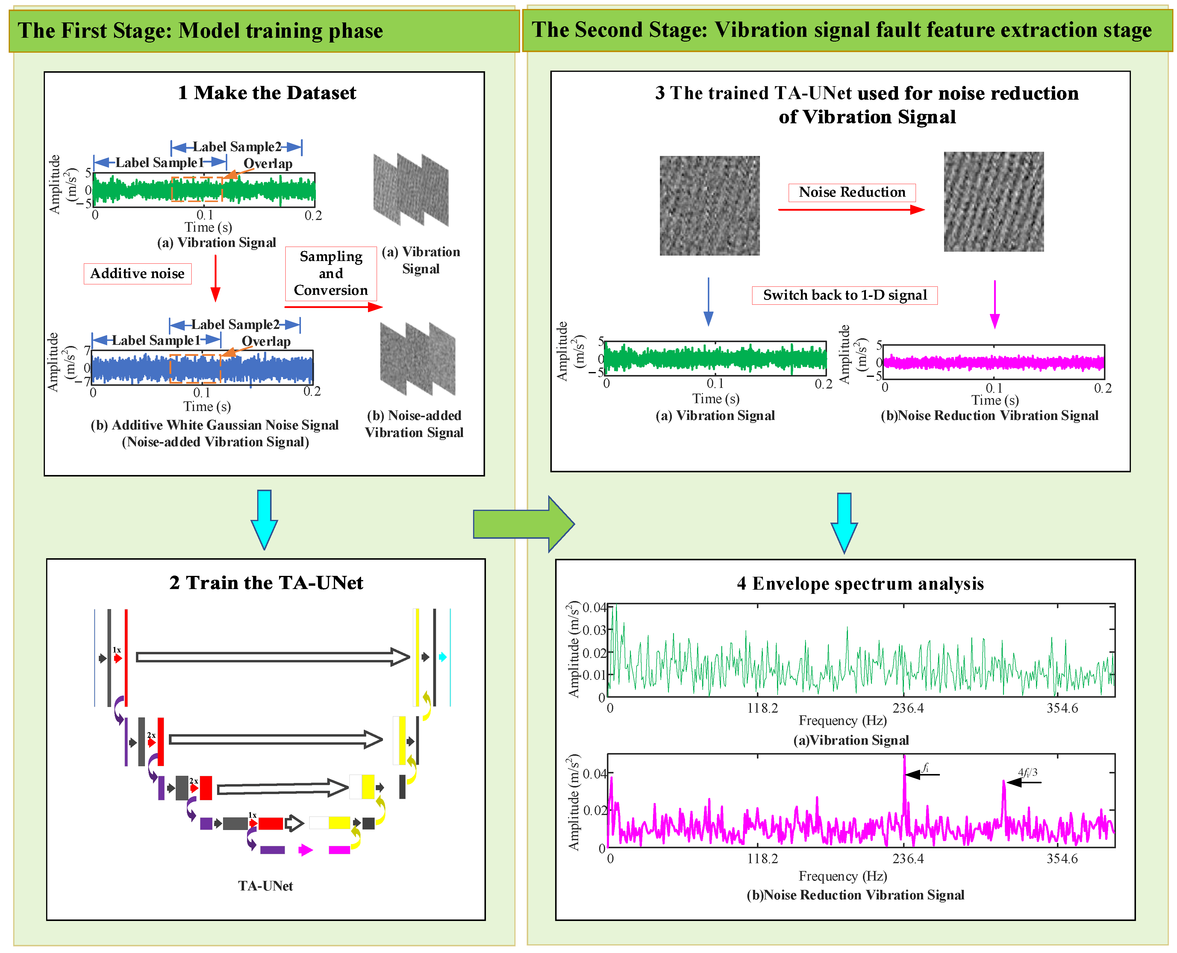
2.4. Early Fault Diagnosis Method of Rolling Bearing

Figure 4 shows the dimension reduction of six vibration signals and their implicit feature by t-SNE [41]. In this paper, 3 types of 6 vibration signals are randomly selected, including vibration signal V₁ and its noise-added vibration signal with SNR = −5 dB (V₁-5) and SNR = −10 dB (V₁-10), vibration signal V₂ and its noise-added vibration signal with SNR = −5 dB (V₂-5) and vibration signal V₃. As shown in Figure 4a, t-SNE is used to reduce the dimensions of the above six vibration signals directly, and then the results are visualized. It was found that the signals were clustered together, and the relationship between signals could not be distinguished. As shown in Figure 4b, this paper uses CNN to extract the hidden features of six vibration signals, reduce the dimensions of the hidden features, and then visualize the results. It was found that the signals were clustered into three categories, and the aggregated categories were consistent with the actual categories of the signals. Thus, we consider that the vibration signal and noise-added vibration signal have a certain invariance in the hidden characteristics, as shown in Equation (14).

$$F_{Conv2d}\left(X\right)\to F_{Conv2d}^{\prime }\left(X\right)=F_{Conv2d}^{\prime }\left(X_N\right)\leftarrow F_{Conv2d}\left(X_N\right)$$

(14)

where X is the vibration signal, and X_N is the noisy vibration signal, $F_{Conv2d}\left(X\right)$ and $F_{Conv2d}\left(X_N\right)$ denote the implicit features of the signals, and $F_{Conv2d}^{\prime }\left(X\right)$ = $F_{Conv2d}^{\prime }\left(X_N\right)$ denotes the invariant content of the implicit feature of the vibration signal X and the noise-added vibration signal X_N.

Figure 5 shows the fault diagnosis method of rolling bearing proposed in this paper. In this paper, using the excellent feature extraction ability of TA-UNet and the invariance of the implicit feature of vibration and noisy vibration signals, a fault diagnosis method of rolling bearing based on TA-UNet is proposed.

The fault diagnosis method is divided into two stages. In the first stage, the vibration signal and vibration signal with additive white gaussian noise (noise-added vibration signal) are sampled by sliding window and then the sample is converted into the gray matrix to make the dataset. Finally, the dataset is used to train the TA-UNet, so it can learn to extract the hidden feature of the noise-added vibration signal and realize the noise-reduced vibration signal. Because the implicit features of vibration and noise-added vibration signal have certain invariances, this paper believes that the network has learned how to extract the implicit feature of vibration signals (how to reduce the noise of vibration signals) to a certain extent. In the second stage, the trained network is used to reduce the noise of the vibration signal, and envelope spectrum analysis of the noise-reduced vibration signal is conducted to diagnose bearing faults. The fault diagnosis method can be expressed by Equation (15).

$$F_{TA}\left(X_N\right)\to F_{TA}^{\prime }\left(X\right)$$

(15)

where $F_{TA}\left(X_N\right)$ denotes the noise reduction of the noisy vibration signal by the TA-UNet, $F_{TA}^{\prime }\left(X\right)$ denotes the noise reduction of the vibration signal by the trained TA-UNet.

3. Validation of TA-UNet Noise Reduction Capability

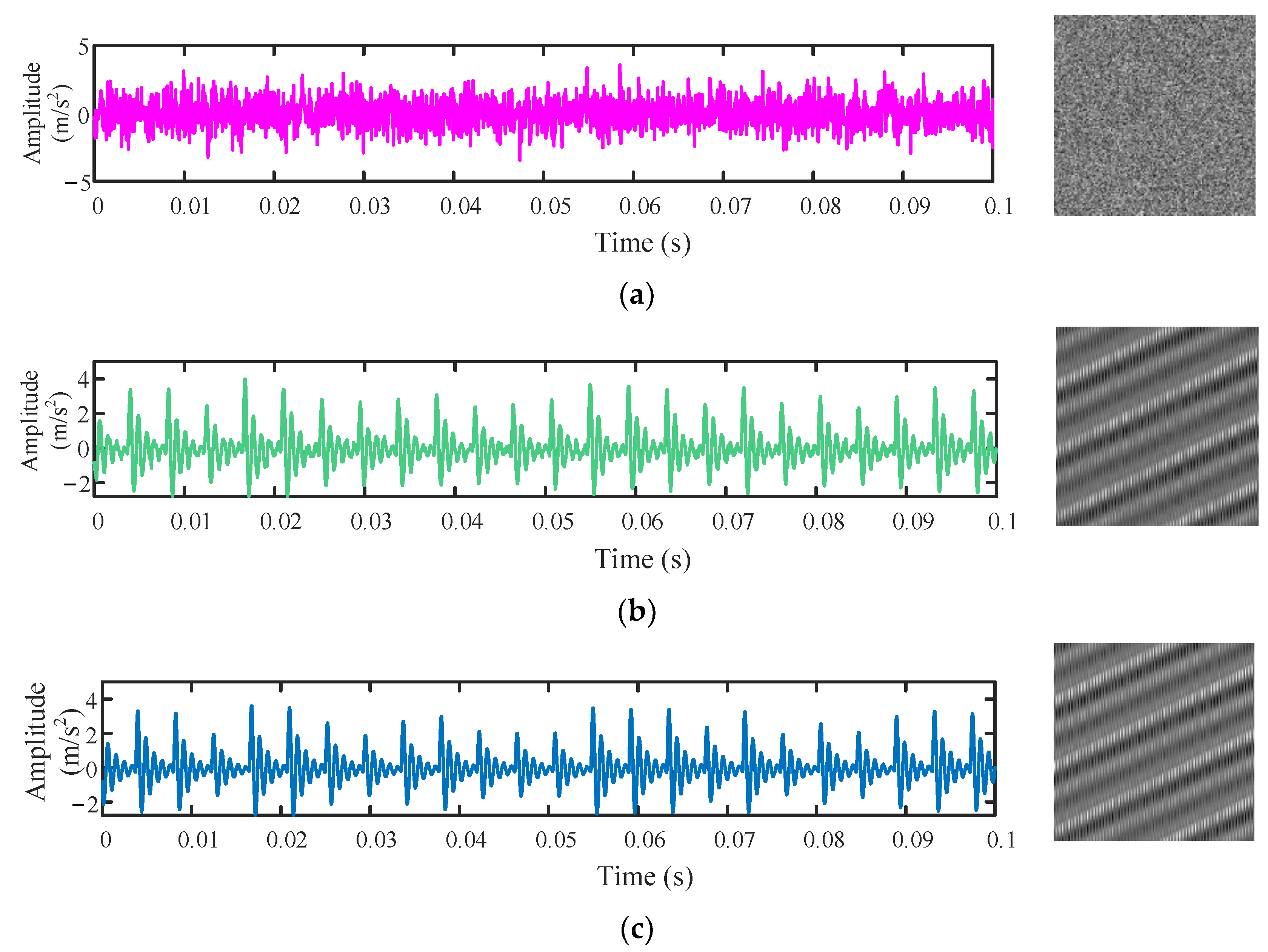
3.1. The Dataset of the Simulation Signal

To verify the noise reduction capability of the TA-UNet, this paper uses a fault model to simulate the impact signal of the bearing outer ring fault, as shown in Equation (16). Firstly, the impact signal is sampled by a sliding window with a step size of 1800. Each sample contains 16,384 sampling points, and the number of samples is 300. Then, the noise was added to the 300 samples to simulate the early fault simulation signal of the bearing outer ring. Finally, the 1-D signal was converted to 128 × 128 and was divided into training, validation, and tests set according to the proportion of 5:3:2.

$$\left.\begin{array}{l}x\left(t\right)=s\left(t\right)+n\left(t\right)={\displaystyle \sum _i{A}_{i}h\left(t-iT-{\tau }_i\right)+n\left(t\right)}\\ h\left(t\right)=e^{-Ct}\sin \left(2\pi f_{n}t\right)\\ A_i=1+A_0\sin \left(2\pi f_{n}t\right)\end{array}\right\}$$

(16)

where s(t) is the periodic impact signal, n(t) is gaussian white noise, x(t) is the simulation signal, A₀ = 0.3 is the initial value of amplitude, f_n = 20 Hz is the rotational frequency, C = 700 is the attenuation coefficients, f₀ = 3000 Hz is the resonant frequency, f_i = 1/T = 80 Hz is the feature frequency of outer ring fault, f_s = 20 kHz is the sampling frequency, and the sampling time lasts for 50 s.

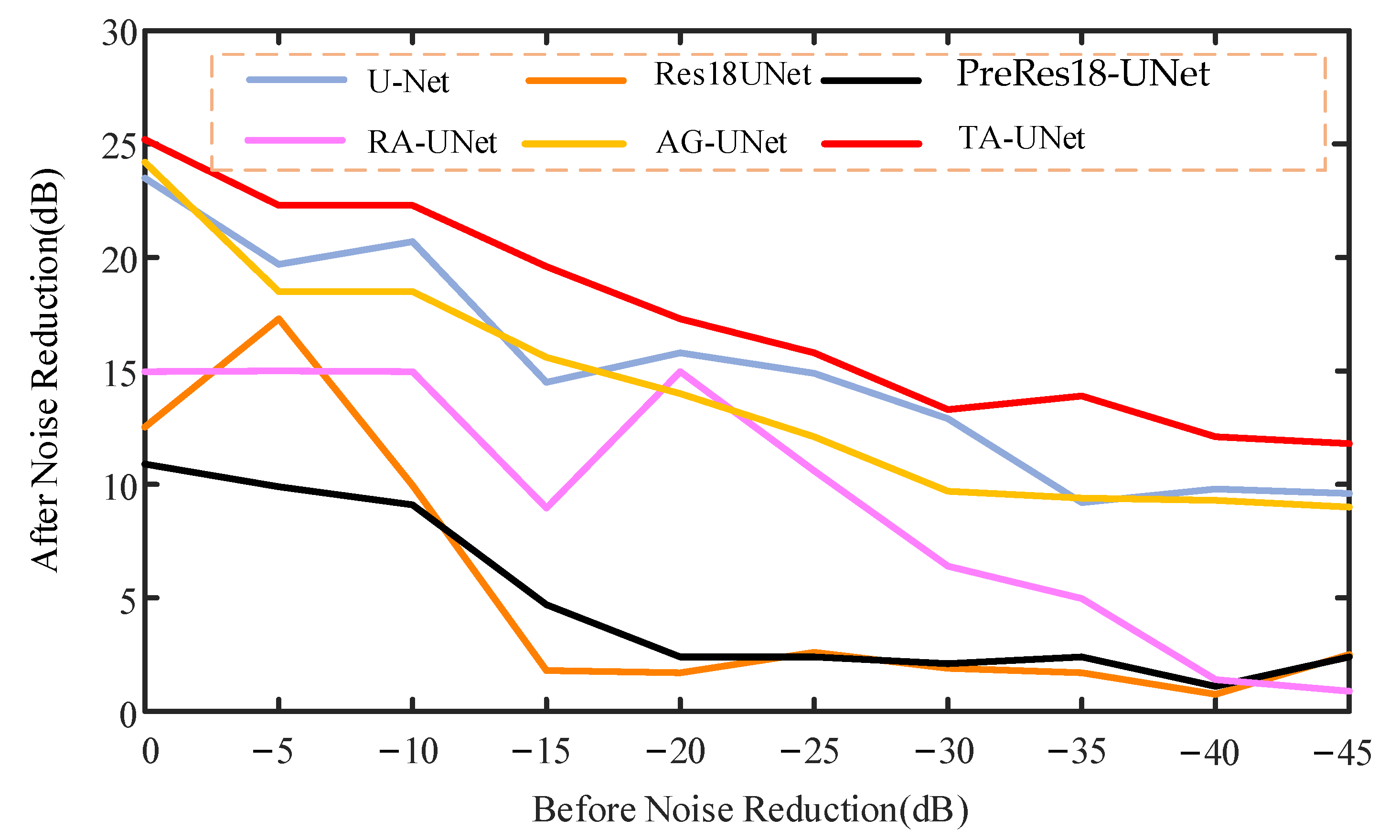
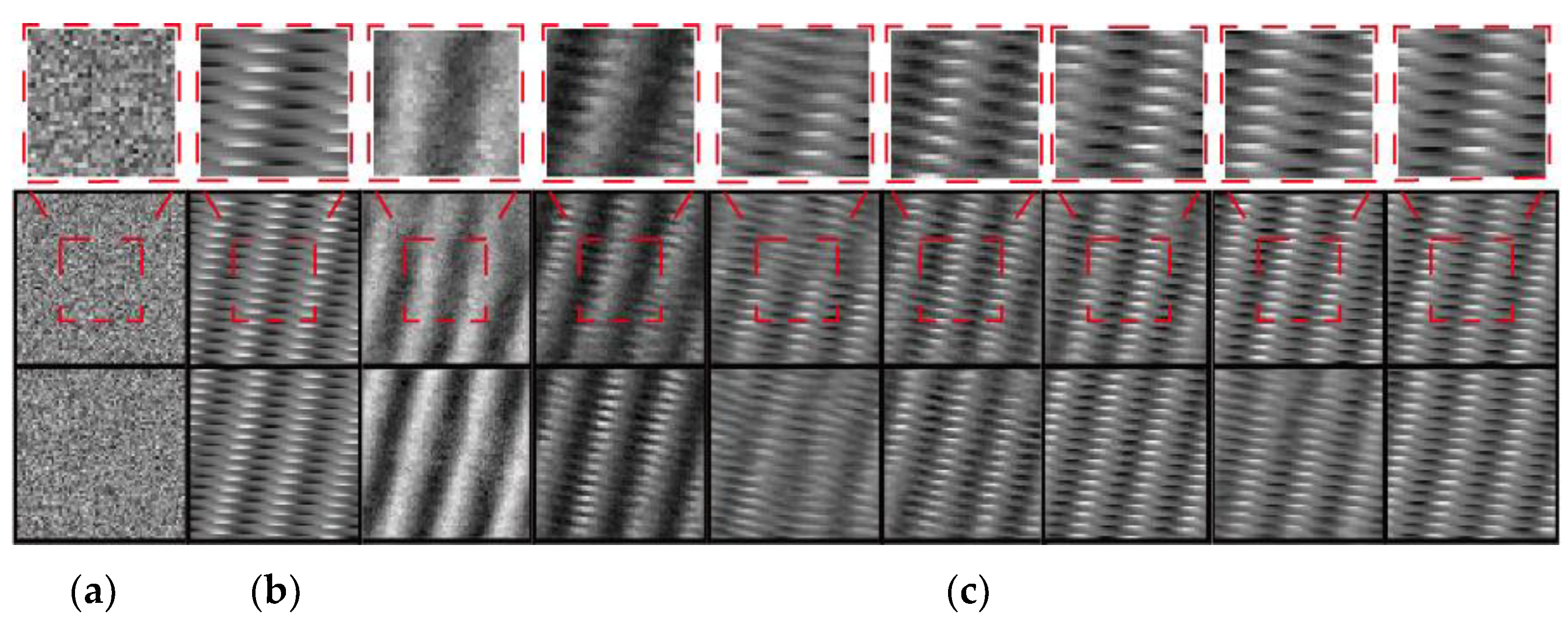
3.2. Comparison of Noise Reduction Results

Figure 6 shows the result of the TA-UNet noise reduction for simulation signals with SNR = −45 dB. During the training stage, this paper uses the training samples mentioned in Section 3.1 as the training set and standardizes the data. The networks are optimized using the Adam gradient descent algorithm, and this paper sets the decay rates β₁ = 0.6 and β₂ = 0.9 and batch size = 32. This paper set the learning rate = 0.0002 and the training epoch = 100. During the testing stage, the network was tested through the test samples mentioned in Section 3.1 and the network noise reduction effect was evaluated through the SNR of the noise reduction signal. The SNR calculation method is shown in Equation (17). Figure 6 shows this paper’s selection of 2000 points of one of the results. The TA-UNet reverts to the periodic impact signal after noise reduction of the simulation signal with SNR = −45 dB, and the SNR of the noise reduction signal was 13.6 dB.

$$SNR=10\lg \left(\frac{{\displaystyle \sum _{i=1}^{n}x{\left(t\right)}^2}}{{\displaystyle \sum _{i=1}^n{\left(x\left(t\right)-x^{\prime }\left(t\right)\right)}^2}}\right)\left(dB\right)$$

(17)

where x(t) is the original signal, x′(t) is the signal after noise reduction, and n is the signal length.

Figure 7 shows the noise reduction effect of different models on different SNR simulation signals. To further verify the noise reduction capability of the TA-UNet in this paper, the TA-UNet was used to reduce the noise of simulation signals with SNR from 0 dB to −45 dB and compared with different networks, including U-Net, Res18-UNet [42], PreRes18-UNet, RA-UNet [43], and AG-UNet [44]. We chose the same training set and experimental setting for all approaches during the training stage. During the test stage, each model randomly selected five training results for the test set, tested 32 samples each time, calculated the average SNR, and compared the noise reduction effect of different models.

Figure 8 shows the process of the TA-UNet noise reduction for SNR = −45 dB simulation signal, with an epoch from 10 to 100. To further understand the performance of the TA-UNet, this paper analyzed the process of the TA-UNet noise reduction for the simulated signal with SNR = −45 dB. As shown in Figure 8, when epoch = 40, the basic waveform was recovered, but the details were lacking, so we continued to train the network. When epoch = 80, the noise reduction effect was already excellent. Therefore, to further improve the stability of the network, 20 epochs were trained.

4. Verification of Diagnostic Method

4.1. Case 1

The open-source dataset one is used in Case 1, as shown in Figure 9 [45]. In dataset one, the four Rexnord ZA-2115 double-row bearings were in the same shaft. A radial load of 6000 pounds was applied to the shaft and bearing. Simultaneously, an acceleration sensor was installed in the axial direction and radial direction of each bearing. The motor speed was 2000 r/min, data were collected every 10 min, 20,480 points were collected each time, and the sampling frequency was 20 kHz. The test ended when the outer ring of bearing 1 failed completely. Case 1 used the vibration data of bearing 1 for analysis and research, and the fault frequency of the outer ring f_i was 236.43 Hz.

Figure 10 shows the root mean square (RMS) trend of bearing vibration signal in Case 1. The trend of RMS reflects the whole process of the bearing operation. As shown in Figure 10, the bearing runs relatively stably before 5320 min. When operating at 5320 min, the RMS slowly rose after a slight mutation, indicating that the bearing status was abnormal. At 7020 min, the RMS had a large jump, indicating that the fault was aggravated, and reached the maximum at 9790 min, at which the bearing had reached the service life limit.

To evaluate the method proposed in this paper, Case 1 selected vibration signals from 5100 min to 5200 min for early fault diagnosis. First, the method mentioned in Section 3.1 was used to make a dataset for the selected data, and then we trained the network to learn to reduce the noise of noise-added vibration signal. Then, the trained network was applied to the selected data, and the noise reduction signal was obtained after noise reduction. Finally, the envelope spectrum of the noise reduction signal was analyzed to diagnose the fault type.

For Case 1, considering that the fault characteristic of the vibration signal is relatively weak and basically drowned out by noise, the SNRs of the noise-added vibration signal used for TA-UNet training were set to −10 dB, −15 dB, −20 dB, and −25 dB. Through this operation, the number of fault characteristics in the vibration signal to be processed by the trained TA-UNet can be informed in advance: weak, which can further improve the feature extraction ability of the trained TA-UNet on the vibration signal. The trained TA-UNet obtained by using the above three noise-added vibration signals was applied to the vibration signal, respectively, and the effect of feature extraction was compared. In Case 1, the SNR = −20 dB noise-added vibration signal was finally chosen.

Figure 11 shows the waveform and the envelope spectrum of the vibration signal and noise-reduced vibration signal in Case 1. As shown in Figure 11a, it can be seen from the waveforms of the two signals that the vibration signal has been denoised. To more accurately prove that the vibration signal has been denoised, the index of vibration signal entropy is selected in this paper. Entropy is an indicator that can reflect the complexity and randomness of the signal. The lower the entropy, the higher the certainty of the signal, that is, the less noise the signal contains. In this paper, three common entropies are selected: approximate entropy, fuzzy entropy, and sample entropy.

Table 1. Entropy values of vibration and noise reduction signal in Case 1.

	Approximate Entropy	Sample Entropy	Fuzzy Entropy
The vibration signal	2.029	1.936	0.193
The noise-reduced vibration signal	1.473	1.346	0.170
The amount of the decrease in entropy after the signal is denoised	27.4%	30.4%	12.0%

shows the approximate entropy, sample entropy, and fuzzy entropy of the vibration signal and the noise reduction vibration signal in Case 1. The entropy values of the noise-reduced vibration signal decreased by 27.4%, 30.4%, and 12.0%, respectively, indicating that the noise-reduced vibration signal was more deterministic, suggesting that the vibration signal was denoised.

As shown in Figure 11b, the envelope spectrum of the vibration signal was observed, and the frequency was found to be disordered. The fault feature frequency f_i components were not obvious, so the bearing fault could not be diagnosed. As shown in Figure 11c, the envelope spectrum of the noise-reduced vibration signal shows prominent components f_i/3, 2f_i/3, f_i, 5f_i/3, and 7f_i/3 related to the fault frequency f_i of the outer ring. The theory is consistent with the practice, which proves the effectiveness of the fault diagnosis method proposed in this paper, and the bearing fault was found 2 h earlier than with the RMS method.

Figure 12 shows the envelope spectrum of the noise reduction vibration signal obtained by EEMD, VMD, WPD, and the proposed method in Case 1. To highlight the advantages of the proposed method, several common vibration signal feature extraction methods are selected for comparison with the proposed method, including EEMD, VMD, and WPD. For EEMD and VMD, after obtaining IMFs, this paper selects appropriate IMFs for reconstruction through the correlation coefficient method and determines the number of WPD decomposition layers according to sample entropy. The noise reduction signals are analyzed by envelope spectrum, and the results are shown in Figure 12. From the figure, it is obvious to see the superiority of the proposed method.

Figure 13 shows the envelope spectrum of vibration signal and different noise-canceling vibration signals in Case 1. As shown in Figure 13, to further verify the feature extraction ability of the TA-UNet, the three networks with the highest noise reduction ability in Section 3 are selected, the TA-UNet, the U-Net, and the AG-UNet, to use the fault diagnosis method proposed in this article to diagnose the early fault of rolling bearing. It can be found that the U-Net and the AG-UNet can extract the fault characteristics of rolling bearings to a certain extent, but the ability to extract fault features is weak. The above two networks are prone to misjudgment compared with the TA-UNet. Figure 13 can prove the feature extraction ability of the TA-UNet and the effectiveness of the fault diagnosis method in this paper.

4.2. Case 2

The open-source dataset two was used in Case 2, as shown in Figure 14 [46]. The vibration data in the horizontal direction of a bearing with an inner ring fault was adopted in Case 2, whose speed was 2400 r/min, a radial force of 10 kN was applied, and the bearing ran for 25 h 15 min until it completely failed. Notably, the fault type was the bearing with an inner ring fault. The fault feature frequency of the bearing inner f_i is 196.8 Hz.

Figure 15 shows the RMS trend of the vibration signal in Case 2. As shown in Figure 15, since 990 min, there has been a significant fluctuation in the RMS, which indicates that the rolling bearing had started to appear abnormal. In Case 2, signals from 900 to 910 min were selected to diagnose the early fault of the rolling bearing, and the SNR = −20 dB noise-added vibration signal was finally chosen.

Figure 16 shows the waveform and envelope spectrum of the bearing vibration signal before and after noise reduction in Case 2. As shown in Figure 16a, the waveforms of the two signals were observed, and the vibration signal was denoised.

As shown in

Table 2. Entropy values of vibration and noise reduction signal in Case 2.

	Approximate Entropy	Sample Entropy	Fuzzy Entropy
The vibration signal	2.211	2.171	0.161
The noise-reduced vibration signal	1.964	1.852	0.141
The amount of the decrease in entropy after the signal is denoised	11.2%	15.0%	12.4%

, the approximate entropy, sample entropy and fuzzy entropy before and after signal noise reduction are calculated, and after noise reduction, it is reduced by 11.2%, 15.0%, and 12.4%, respectively, indicating that the signal is denoised.

As shown in Figure 16b,c, compared with the vibration signal, the noise-reduced vibration signal envelope spectrum showed an obvious 0.5×, 1×, and 1.5× feature frequency related to the inner ring fault feature frequency f_i. Figure 16 further verified the superiority of the early diagnosis method for rolling bearings proposed in this paper, and the bearing fault was found 1.3 h earlier than with the RMS method.

Figure 17 shows the envelope spectrum of different noise-canceling vibration signals in Case 2. As shown in Figure 17, like Figure 12, the effectiveness of the TA-UNet’s feature extraction ability and fault diagnosis method proposed in this paper can be further demonstrated. The superiority of the proposed method is further demonstrated.

Figure 18 shows the envelope spectrum of vibration signal and different noise-canceling vibration signals in Case 2. As shown in Figure 18, similar to Figure 13, the effectiveness of the TA-UNet’s feature extraction ability and fault diagnosis method proposed in this paper can be further demonstrated.

5. Conclusions

A two-stage method of the early fault diagnosis of rolling bearing based on the TA-UNet is proposed to improve the accuracy of early fault diagnoses of rolling bearing.

First, based on the U-Net, the TA-UNet is proposed by combining the CS-TAN and the DCM. The CS-TAN reduces the noise interference in the signal during the down-sampling, and the DCM improves its multi-scale feature extraction capability. This paper proves that the TA-UNet has super noise reduction ability by reducing the noise of simulation signals of different SNRs and is superior to the typical deep learning model in performance. For the simulation signal with SNR = −45 dB, the SNR of the simulation signal after the TA-UNet noise reduction reached 13.6 dB, which was 2 dB higher than that of the U-Net and 1 dB higher than that of the AG-UNet.

Second, the TA-UNet is used to diagnose the early fault of the rolling bearing by its strong feature extraction ability and the invariance of the implied feature of vibration signal and noise-added vibration signal. The early fault types of Case 1 and Case 2 are successfully diagnosed, which proved the method’s effectiveness, and were 2 h and 1.3 h ahead of the RMS method, respectively.

In summary, this study reveals a new method for bearings’ fault detection. Future work will focus on how to improve the speed of diagnosis and expand this work to more application scenarios.

References

1. Gu, R.; Chen, J.; Hong, R.; Wang, H.; Wu, W. Incipient fault diagnosis of rolling bearings based on adaptive variational mode decomposition and Teager energy operator. Measurement 2020, 149, 106941. [Google Scholar] [CrossRef]
2. Ren, X.; Zhang, Y.; Xing, Y.; Wang, C. Rolling bearing early fault diagnosis based on angular domain cascade maximum correlation kurtosis deconvolution. Chin. J. Sci. Instrum. 2015, 36, 2104–2111. (In Chinese) [Google Scholar]
3. Pang, B.; Tian, T.; Tang, G.J. Fault state recognition of wind turbine gearbox based on generalized multi-scale dynamic time warping. Struct. Health Monit. 2021, 20, 3007–3023. [Google Scholar] [CrossRef]
4. Harmouche, J.; Delpha, C.; Diallo, D. Improved Fault Diagnosis of Ball Bearings Based on the Global Spectrum of Vibration Signals. IEEE Trans. Energy Convers. 2015, 30, 376–383. [Google Scholar] [CrossRef]
5. Zhang, K.; Tang, B.; Deng, L.; Tan, Q.; Yu, H. A fault diagnosis method for wind turbines gearbox based on adaptive loss weighted meta-ResNet under noisy labels. Mech. Syst. Signal Process. 2021, 161, 107963. [Google Scholar] [CrossRef]
6. Feng, K.; Ji, J.C.; Ni, Q.; Beer, M. A review of vibration-based gear wear monitoring and prediction techniques. Mech. Syst. Signal Process. 2023, 182, 109605. [Google Scholar] [CrossRef]
7. Lu, P.; Powrie, H.E.; Wood, R.J.; Harvey, T.J.; Harris, N.R. Early wear detection and its significance for condition monitoring. Tribol. Int. 2021, 159, 106946. [Google Scholar] [CrossRef]
8. Zhang, H.; Ma, J.; Li, X.; Xiao, S.; Gu, F.; Ball, A. Fluid-asperity interaction induced random vibration of hydrodynamic journal bearings towards early fault diagnosis of abrasive wear. Tribol. Int. 2021, 160, 107028. [Google Scholar] [CrossRef]
9. Li, Y.; Yang, Y.; Wang, X.; Liu, B.; Liang, X. Early fault diagnosis of rolling bearings based on hierarchical symbol dynamic entropy and binary tree support vector machine. J. Sound Vib. 2018, 428, 72–86. [Google Scholar] [CrossRef]
10. Yu, D.; Cheng, J.; Yang, Y. Application of EMD method and Hilbert spectrum to the fault diagnosis of roller bearings. Mech. Syst. Signal Process. 2005, 19, 259–270. [Google Scholar] [CrossRef]
11. Guo, J.; Zhen, D.; Li, H.; Shi, Z.; Gu, F.; Ball, A.D. Fault feature extraction for rolling element bearing diagnosis based on a multi-stage noise reduction method. Measurement 2019, 139, 226–235. [Google Scholar] [CrossRef]
12. Liu, W.Y.; Gao, Q.W.; Ye, G.; Ma, R.; Lu, X.N.; Han, J.G. A novel wind turbine bearing fault diagnosis method based on Integral Extension LMD. Measurement 2015, 74, 70–77. [Google Scholar] [CrossRef]
13. Xiong, G.; Przystupa, K.; Teng, Y.; Xue, W.; Huan, W.; Feng, Z.; Qiong, X.; Wang, C.; Skowron, M.; Kochan, O.; et al. Online Measurement Error Detection for the Electronic Transformer in a Smart Grid. Energies 2021, 14, 3551. [Google Scholar] [CrossRef]
14. Ni, Q.; Ji, J.C.; Feng, K.; Halkon, B. A fault information-guided variational mode decomposition (FIVMD) method for rolling element bearings diagnosis. Mech. Syst. Signal Process. 2022, 164, 108216. [Google Scholar] [CrossRef]
15. Pang, B.; Nazari, M.; Tang, G. Recursive variational mode extraction and its application in rolling bearing fault diagnosis. Mech. Syst. Signal Process. 2022, 165, 108321. [Google Scholar] [CrossRef]
16. Lu, G.; Wen, X.; He, G.; Yi, X.; Yan, P. Early Fault Warning and Identification in Condition Monitoring of Bearing via Wavelet Packet Decomposition Coupled with Graph. IEEEASME Trans. Mechatron. 2022, 27, 3155–3164. [Google Scholar] [CrossRef]
17. Gunawan, R.; Tran, Y.; Zheng, J.; Nguyen, H.; Chai, R. Image Recovery from Synthetic Noise Artifacts in CT Scans Using Modified U-Net. Sensors 2022, 22, 7031. [Google Scholar] [CrossRef] [PubMed]
18. Tan, H.; Ou, D.; Zhang, L.; Shen, G.; Li, X.; Ji, Y. Infrared Sensation-Based Salient Targets Enhancement Methods in Low-Visibility Scenes. Sensors 2022, 22, 5835. [Google Scholar] [CrossRef]
19. Kim, D.W.; Ryun Chung, J.; Jung, S.W. GRDN: Grouped Residual Dense Network for Real Image Denoising and GAN-Based Real-World Noise Modeling. In Proceedings of the 2019 IEEE/CVF Conference on Computer Vision and Pattern Recognition Workshops (CVPRW), Long Beach, CA, USA, 15–20 June 2019; pp. 2086–2094. [Google Scholar]
20. LeCun, Y.; Bengio, Y.; Hinton, G. Deep learning. Nature 2015, 521, 436–444. [Google Scholar] [CrossRef]
21. O’Shea, K.; Nash, R. An introduction to convolutional neural networks. arXiv 2015, arXiv:1511.08458. [Google Scholar]
22. Gong, L.; Fan, S. A CNN-Based Method for Counting Grains within a Panicle. Machines 2022, 10, 30. [Google Scholar] [CrossRef]
23. Piratelo, P.H.M.; de Azeredo, R.N.; Yamao, E.M.; Bianchi Filho, J.F.; Maidl, G.; Lisboa, F.S.M.; de Jesus, L.P.; Penteado Neto, R.D.A.; Coelho, L.D.S.; Leandro, G.V. Blending Colored and Depth CNN Pipelines in an Ensemble Learning Classification Approach for Warehouse Application Using Synthetic and Real Data. Machines 2021, 10, 28. [Google Scholar] [CrossRef]
24. Ronneberger, O.; Fischer, P.; Brox, T. U-Net: Convolutional Networks for Biomedical Image Segmentation. In Proceedings of the Medical Image Computing and Computer-Assisted Intervention. In MICCAI 2015; Springer: Cham, Switzerland, 2015; pp. 234–241. [Google Scholar]
25. Cai, S.; Tian, Y.; Lui, H.; Zeng, H.; Wu, Y.; Chen, G. Dense-UNet: A novel multiphoton in vivo cellular image segmentation model based on a convolutional neural network. Quant. Imaging Med. Surg. 2020, 10, 1275–1285. [Google Scholar] [CrossRef]
26. Feng, C.; Zhang, H.; Wang, H.; Wang, S.; Li, Y. Automatic Pixel-Level Crack Detection on Dam Surface Using Deep Convolutional Network. Sensors 2020, 20, 2069. [Google Scholar] [CrossRef] [PubMed] [Green Version]
27. Qiu, L.; Cai, W.; Yu, J.; Zhong, J.; Wang, Y.; Li, W.; Chen, Y.; Wang, L. A two-stage ECG signal denoising method based on deep convolutional network. bioRxiv 2020, 2020.03.27.012831. [Google Scholar] [CrossRef]
28. Stoller, D.; Ewert, S.; Dixon, S. Wave-u-net: A multi-scale neural network for end-to-end audio source separation. arXiv 2018, arXiv:1806.03185. [Google Scholar]
29. Hao, X.; Su, X.; Wang, Z.; Zhang, H. UNetGAN: A Robust Speech Enhancement Approach in Time Domain for Extremely Low Signal-to-noise Ratio Condition. In Proceedings of the Interspeech 2019, Graz, Austria, 15–19 September 2019; pp. 1786–1790. [Google Scholar]
30. Shang, Z.; Sun, L.; Xia, Y.; Zhang, W. Vibration-based damage detection for bridges by deep convolutional denoising autoencoder. Struct. Health Monit. 2021, 20, 1880–1903. [Google Scholar] [CrossRef]
31. Yu, K.; Fu, Q.; Ma, H.; Lin, T.R.; Li, X. Simulation data driven weakly supervised adversarial domain adaptation approach for intelligent cross-machine fault diagnosis. Struct. Health Monit. 2021, 20, 2182–2198. [Google Scholar] [CrossRef]
32. Wen, L.; Gao, L.; Li, X. A New Deep Transfer Learning Based on Sparse Auto-Encoder for Fault Diagnosis. IEEE Trans. Syst. Man Cybern. Syst. 2019, 49, 136–144. [Google Scholar] [CrossRef]
33. Wang, X.; Shen, C.; Xia, M.; Wang, D.; Zhu, J.; Zhu, Z. Multi-scale deep intra-class transfer learning for bearing fault diagnosis. Reliab. Eng. Syst. Saf. 2020, 202, 107050. [Google Scholar] [CrossRef]
34. Zhang, Y.; Ren, Z.; Zhou, S.; Feng, K.; Yu, K.; Liu, Z. Supervised Contrastive Learning-Based Domain Adaptation Network for Intelligent Unsupervised Fault Diagnosis of Rolling Bearing. IEEEASME Trans. Mechatron. 2022, 27, 5371–5380. [Google Scholar] [CrossRef]
35. Zhao, M.; Zhong, S.; Fu, X.; Tang, B.; Pecht, M. Deep Residual Shrinkage Networks for Fault Diagnosis. IEEE Trans. Ind. Inform. 2020, 16, 4681–4690. [Google Scholar] [CrossRef]
36. Donoho, D.L. De-noising by soft-thresholding. IEEE Trans. Inf. Theory 1995, 41, 613–627. [Google Scholar] [CrossRef]
37. Yang, J.; Zhu, J.; Wang, H.; Yang, X. Dilated MultiResUNet: Dilated multiresidual blocks network based on U-Net for biomedical image segmentation. Biomed. Signal Process. Control 2021, 68, 102643. [Google Scholar] [CrossRef]
38. Yu, F.; Koltun, V. Multi-scale context aggregation by dilated convolutions. arXiv 2015, arXiv:1511.07122. [Google Scholar]
39. Huang, W.; Yin, G.; Geng, K. Object detection in complex driving scene based on dilated convolution feature adaptive fusion. J. Southeast Univ. Nat. Sci. Ed. 2021, 51, 1076–1083. [Google Scholar]
40. Odena, A.; Dumoulin, V.; Olah, C. Deconvolution and Checkerboard Artifacts. Distill 2016, 1, e3. [Google Scholar] [CrossRef]
41. Van der Maaten, L.; Hinton, G. Visualizing data using t-SNE. J. Mach. Learn. Res. 2008, 9, 2579–2605. [Google Scholar]
42. Stephan, M.; Santra, A. Radar-based Human Target Detection using Deep Residual U-Net for Smart Home Applications. In Proceedings of the 2019 18th IEEE International Conference on Machine Learning and Applications (ICMLA), Boca Raton, FL, USA, 16–19 December 2019; pp. 175–182. [Google Scholar] [CrossRef]
43. Jin, Q.; Meng, Z.; Sun, C.; Cui, H.; Su, R. RA-UNet: A hybrid deep attention-aware network to extract liver and tumor in CT scans. Front. Bioeng. Biotechnol. 2020, 8, 605132. [Google Scholar] [CrossRef]
44. Yin, Y.; Xu, D.; Wang, X.; Zhang, L. AGUnet: Annotation-guided U-net for fast one-shot video object segmentation. Pattern Recognit. 2021, 110, 107580. [Google Scholar] [CrossRef]
45. Yu, J. Health Condition Monitoring of Machines Based on Hidden Markov Model and Contribution Analysis. IEEE Trans. Instrum. Meas. 2012, 61, 2200–2211. [Google Scholar] [CrossRef]
46. Wang, B.; Lei, Y.; Li, N.; Li, N. A Hybrid Prognostics Approach for Estimating Remaining Useful Life of Rolling Element Bearings. IEEE Trans. Reliab. 2020, 69, 401–412. [Google Scholar] [CrossRef]
Figure 1. Structure of channel threshold acquisition network (C-TAN) and channel spatial threshold acquisition network (CS-TAN). (a) Structure of C-TAN; (b) Structure of CS-TAN.
Machines 11 00119 g001
Figure 2. Dilated convolution module with exponentially increasing dilated rate (r = 1, 2, 4), stride = 1, kernel size = 3.
Machines 11 00119 g002
Figure 3. Structure of the proposed TA-UNet.
Machines 11 00119 g003
Figure 4. t-SNE reduces the dimension of the vibration signal and the implicit feature of the vibration signal. (a) t-SNE reduces the dimension of the vibration signal; (b) t-SNE reduces the dimension of the implicit feature of the vibration signal.
Machines 11 00119 g004
Figure 5. Early fault diagnosis method of rolling bearing based on TA-UNet.
Machines 11 00119 g005
Figure 6. TA-UNet noise reduction results for simulation signal with SNR = −45 dB. (a) Simulation signal with SNR = −45 dB; (b) Noise reduction results of simulation signal by TA-UNet; (c) Impulse signal.
Machines 11 00119 g006
Figure 7. Noise reduction results of different networks for different SNRs.
Machines 11 00119 g007
Figure 8. Training Process of TA-UNet for SNR = −45 dB simulation signal noise reduction. (a) outer fault impulse signal; (b) simulation signal with SNR = −45 dB; (c) training process of TA-UNet, epochs are 10 in turn, 20, 30, 40, 60, 80, 100 (from left to right).
Machines 11 00119 g008
Figure 9. The layout of the bearing accelerated degradation test rig of Case 1.
Machines 11 00119 g009
Figure 10. The RMS trend of bearing vibration signal in Case 1.
Machines 11 00119 g010
Figure 11. Waveform and envelope spectrum of vibration signal and noise-reduced vibration signal in Case 1. (a) Waveform of vibration signal and noise-reduced vibration signal; (b) Envelope spectrum of vibration signal; (c) Envelope spectrum of noise reduction signal.
Machines 11 00119 g011
Figure 12. The envelope spectrum of the noise reduction vibration signal obtained by EEMD, VMD, WPD, and the proposed method in Case 1. (a) EEMD; (b) VMD; (c) WPD; (d) The proposed method.
Machines 11 00119 g012
Figure 13. Envelope spectrum of vibration signal and different noise-reduced vibration signals in Case 1. (a) Envelope spectrum of vibration signal; (b) Envelope spectrum of noise-reduced vibration signal by AG-UNet; (c) Envelope spectrum of noise-canceling vibration signal by U-Net; (d) Envelope spectrum of noise-canceling vibration signal by TA-UNet.
Machines 11 00119 g013
Figure 14. The layout of the bearing accelerated degradation test rig of Case 2.
Machines 11 00119 g014
Figure 15. The RMS trend of vibration signal in Case 2.
Machines 11 00119 g015
Figure 16. Waveform and envelope spectrum of vibration signal and noise reduction signal in Case 2. (a) Waveform of vibration signal and noise reduction signal; (b) Envelope spectrum of vibration signal; (c) Envelope spectrum of noise reduction signal.
Machines 11 00119 g016
Figure 17. The envelope spectrum of the noise reduction vibration signal obtained by EEMD, VMD, WPD, and the proposed method in Case 2. (a) EEMD; (b) VMD; (c) WPD; (d) The proposed method.
Machines 11 00119 g017
Figure 18. Envelope spectrum of vibration signal and different noise reduction signals in Case 2. (a) Envelope spectrum of vibration signal; (b) Envelope spectrum of noise reduction signal by AG-UNet; (c) Envelope spectrum of noise reduction signal by U-Net; (d) Envelope spectrum of noise reduction signal by TA-UNet.
Machines 11 00119 g018