Abstract
Small-to-medium sized systems able to perform multiple operations are a promising option for use in agricultural robotics. With this in mind, we present the conceptualization and implementation of a versatile and modular unmanned ground vehicle prototype, which is designed on top of a commercial wheeled mobile platform, in order to test and assess new devices, and motion planning and control algorithms for different Precision Agriculture applications. Considering monitoring, harvesting and spraying as target applications, the developed system utilizes different hardware modules, which are added on top of a mobile platform. Software modularity is realized using the Robot Operating System (). Self- and ambient-awareness, including obstacle detection, are implemented at different levels. A novel extended Boundary Node Method is used for path planning and a modified Lookahead-based Line of Sight guidance algorithm is used for path following. A first experimental assessment of the system’s capabilities in an emulated orchard scenario is presented here. The results demonstrate good path-planning and path-following capabilities, including cases in which unknown obstacles are present.
1. Introduction
In modern agriculture, concepts like precision agriculture, proximal monitoring, and sustainable agriculture are currently important, if not fundamental, for answering the need for increased food production, fighting climate change, and alleviating labor shortages. Indeed, digitalization is impacting agriculture through technologies and advanced data processing techniques for, e.g., land assessment, soil–crop suitability, weather information, crop growth, biomass and productivity, and precision farming [1,2]. It is anticipated that precision agriculture (PA), also known as precision farming or smart farming [3], will increase production with fewer resources by permitting farmers to continuously monitor and manage crops [4]. Therefore, there is a demand for quantitatively establish the effectiveness of in common agricultural applications by testing baseline automated platforms with integrated sensors, controls, information technologies, and algorithms. In this regard, agricultural robotics represents an important part of agri-digitalization [5]. Existing solutions mostly include specialized, task-based, agricultural robots, i.e., robots that can perform a particular task for a specific set of field conditions, but are not suitable for other tasks. Recent literature reports different robotic and mobile robotic applications in agriculture for, e.g., seeding [6], spraying [7], mowing [8], weeding [9,10], pruning [11,12], monitoring and inspection [13,14,15], and harvesting [16]. The existing literature has been reviewed and summarized by [17,18]. Thus, when considering the complexity of agricultural environments resulting from disparate operating conditions, e.g., farm size, orchard topology, and crops, growers must use different machines for different crops and production methods. This is not cost-effective, especially for small farms. To address this issue, some researchers and companies have developed multipurpose robotic platforms that can be used for different production methods [19,20,21,22]. Indeed, reconfigurability and modularization can represent a possible solution when incorporated into the design of field robots [23,24,25,26,27,28,29]. A reconfigurable robot is thus composed of many modules with different functions which can be quickly reconfigured to operate under new circumstances, perform different tasks, or recover from damage [28,29]. In keeping with the philosophy that the whole can be greater than the sum of its parts, individual modules generally have limited sensing, perception, control, computing, and motion capabilities. However, when assembled, the modules should act as a single robotic system. Typically, some sort of uniform docking interface is used between each module to permit the transfer of mechanical power, electrical power, and communication. The complete robot is usually composed of a primary unit, or main platform, and additional specialized modules, such as grippers, wheels, cameras, payload, and energy storage and generation units. Valuable examples of contemporary prototypes and commercial solutions following such an approach are Thorvald [25], MARS [30], GARotics [31], SAGA [32], GRAPE [33], and CATCH [34]. Based on the referenced literature, developing a fully autonomous system like these is still an open research challenge, in particular when the costs and complexity of reconfiguration are considered. By trying to make these platforms useful in numerous tasks such as seeding, spraying, weeding, harvesting, and monitoring, various challenges must be addressed, e.g., harvesting speed, disease detection, path-following/tracking accuracy, field navigation, obstacle avoidance, protection from accidents while operating, human–robot collaboration and multiple-robot collaboration to complete even more complex tasks. Thus, the effective combination of all the involved technologies and the implementation of a complex and extendable infrastructure to support every task of modern cultivation are the results to be targeted.
Therefore, the availability of a modular and reconfigurable platform from the hardware and software point of view in a research lab unlocks the opportunity to also emulate different situations and test different solutions from a basic and applied research standpoint in order to advance the overall state of the art. Indeed, sensors, actuators, and other equipment are needed to experimentally reproduce the main features of different applications (e.g., generating external and interacting forces, creating weight shifts that affect trajectory tracking, localizing the ground vehicle, and permitting safe remote human interaction). The successful integration and implementation of this hardware for applications in precision agriculture requires the development of new algorithms and technical solutions.
In this approach in mind, a reconfigurable system for lab and field activities is conceived in this work starting from hardware already available at the FiRST-Field Robotics South-Tirol Lab of the Free University of Bozen–Bolzano (Italy, see [35]). Regarding the three main configurations and cases related to precision agriculture tasks to be addressed or emulated in the future, i.e., monitoring, harvesting, and spraying, the following considerations and design guidelines have been adopted. Specific functions are enabled using different Hardware () and Software () modules in order that their combination can enhance the functionality of the entire robot, as well as ensure robustness in case of failure, e.g. redundant sensors. Given an orchard scenario, the robot has to be controlled to safely reach goal points, as well as navigate within the rows and the orchard passages; a map-based reliable path planning algorithm that minimizes the distance travelled to reach the goal points must be implemented. Given the fact that the Unmanned Ground Vehicle (UGV) has to maintain a safe distance from obstacles, e.g., trees, the edges of the orchard, fixed and dynamic obstacles, safety-margins and boundary zones must be implemented to allow safe motion of the robot. The UGV system state should be described by its position and orientation (pose) with respect to the environment. Due to the steering mechanism, e.g. skid steering, and environmental characteristics, the wheels are often subjected to slipping and uneven ground that frequently generate disturbances. Since linear and angular speed commands, that can be used separately or combined, are used to actuate the wheels a path-tracking algorithm supported by a proper sensory feedback must be developed and implemented. A combination of feedback navigation sensors is needed for motion control, as well for both self- and ambient-awareness. To act on the environment, manipulation capabilities are to be allowed through at least a 6 degree of freedom manipulator. Finally, good payload capabilities and sufficient clearance between devices must be ensured to accommodate additional modules, or to reconfigure modules for different working scenarios. Overall, the must permit the emulation of sensors, actuators, and other equipment needed to experimentally reproduce the main features of the three test scenarios/applications. At the same time the must support the real-time implementation of: (i) a complete navigation system that can be customized to address the different emulated agricultural scenarios and (ii) a reliable path-following controller.
The main contributions of this work include:
- the functional mechatronic design of a reconfigurable mobile robot to be build on top of an available mobile platform;
- the implementation and prototyping of the modular mechanical and electronic systems based on the design concepts;
- software modules exploiting that can perform automatic tasks combining path planning, obstacle detection, and path-following;
- the implementation of customized path-planning as well as path-following algorithms based on recent literature results;
- preliminary tests of the mobile robot performance in an emulated agricultural scenario.
2. Functional Design Concept and System Configuration
The main platform on which the modular system has been conceived and outfitted for PA is the Husky Unmanned Ground Vehicle (UGV) from Clearpath Robotics, already available at our premises. It presents a skid steering mechanism, which relies on wheel slippage. This simple and robust driving mechanism allows high mobility and assures large traction for manoeuvring on rough surfaces relying on few actuators [36]. On top of it, the proposed functional design concept of hardware and software modules is presented in Figure 1 together with the main flow of information between them. The blocks with the solid line are considered to be standard/required modules. The blocks with a dashed line represent modules that might be added and connected to the main robotic platform, depending on the tasks to be performed. This is conceptualized through the opportunity to add self- and ambient-awareness sensors, a robotic manipulator installed in different locations, a second control box and power unit to extend the robot capabilities, and an adjustable frame to support devices in different ways. As is common in field robotics, the electronic and software architecture of the system are configured so that the high-level control tasks (e.g., path planning, trajectory planning, and task planning and other computationally intensive processes, such as image processing for LiDAR and stereo vision) are separated from low-level control tasks, such as trajectory tracking control, path following control, and state estimation. By doing so the overall control of the mobile platform is more efficient and somewhat modular.
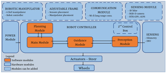
Figure 1.
Functional architecture of the reconfigurable mobile platform. The main modules are depicted in orange. Arrows represent the main flow of information and the communication between modules.
The following subsections introduce and describe the hardware and software modules.
2.1. Configuration
A mobile robotic base represents the ground-layer of the system, and the overall modular platform has been conceived and realized on top. The base is a Husky unmanned ground vehicle (UGV) from Clearpath Robotics. The robot is a four-wheeled skid-steering platform, and it is fully supported by Robot Operating System () [36]. The robot’s main external dimensions are 990 mm in length, 670 mm in width, and 390 mm in height. Its weight is 50 kg, it has a payload of 75 kg, and it can reach a maximum speed of 1 m per second. Two kinds of sensors were integrated with the robot to provide information about the robot’s state in terms of the body’s angular orientation and odometry: onboard wheel encoders with a resolution of 78,000 ticks/m and a CH Robotics UM6 nine-DoF inertial measurement unit (). The latter provides Euler angles with a resolution of 0.01 degree at 500 Hz rate. Several different vehicle configurations were explored to ensure:
- the vision-based systems have good fields-of-view for detecting and then avoiding obstacles, in particular in front of the vehicle, i.e., recognize obstacles to be avoided at a minimum of 2 m in front of the vehicle;
- the robotic manipulator has sufficient clearance over the entire range of its motion, i.e., keep the same footprint, and there would be minimal electronic signal noise from the and WiFi transmitters;
- the positioning systems are appropriately placed to receive satellite and signals, i.e., not occluded or disturbed by other devices.
For the vision-based systems, we adopted a Velodyne VLP-16 LiDAR (range = 100 m, 360 × 30 deg field-of-view, and +/− 15 degree variation) and am Intel Realsense D455 RGB-D camera (range = 0.4 to 6 m, 1280 × 720 resolution, and 86 × 57 degree depth field-of-view).
We decided to mount these devices on a single platform so that they can be rotated together to shift their vertical fields of view. This makes the data more accessible and reliable for both systems by minimizing the amount of re-calibration necessary when repositioning them. Concerning the manipulator, a Universal Robots UR5e manipulator [37] has been considered. As shown in the system layout, it is placed in the front part of the vehicle to ensure adequate clearance. In addition, a pyramid-like structure has been designed for the front of the Husky. The form of this structure permits the base of the robotic manipulator to be mounted in different orientations, which allows us to test our system’s ability to re-tune itself when it is reconfigured automatically. A detailed design configuration for the concept is shown in Figure 2. The designed robot frame (Figure 2) provides the mounting points for all modules. We have decided to use the onboard computer provided with the Husky UGV for the low-level control processes and use a second computer in a newly designed control box (high-level control box) to support electronics. The battery onboard the Husky UGV can provide electrical power to additional sensors that may be required, e.g., LiDAR, stereo camera, and RTK-GPS (outdoor), or ArduSimple simpleRTK2B [38] or iPS (indoor) positioning system, e.g., Pozyx [39]. Fieldwork can severely limit the ability to collect data, as no main power is typically available for recharging. The battery in the second control box is included to increase the time the robot can be operated without needing to stop to recharge. The system can either be run for long periods when attached to the main power line for debugging in the lab or run automatically for several hours in the field. In addition to the batteries, additional connectors, cables, a Ethernet bridge, a USB hub, and RS232 serial interfaces (designed through a set of Arduino Teensy micro-controllers) are used to integrate the high-level computer and different sensors, as well as to interface with the low-level computer in the Husky and the UR5 robotic manipulator. Lastly, an emergency stop push button has been added to ensure that the system can be rapidly disabled during field testing in case of unexpected behavior of the vehicle control system. Block diagrams of the overall electronics configuration and the high-level control box can be seen in Figure 3. In general, the heavy components (i.e., the UR5e manipulator, the UR5e manipulator control box, and the high-level control box with internal batteries) are distributed uniformly across the vehicle. Moreover, the center of gravity is placed as low as possible to maintain the stability of the ground vehicle on sloped terrain.
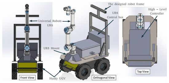
Figure 2.
The design concept of the reconfigurable unmanned ground vehicle (UGV).
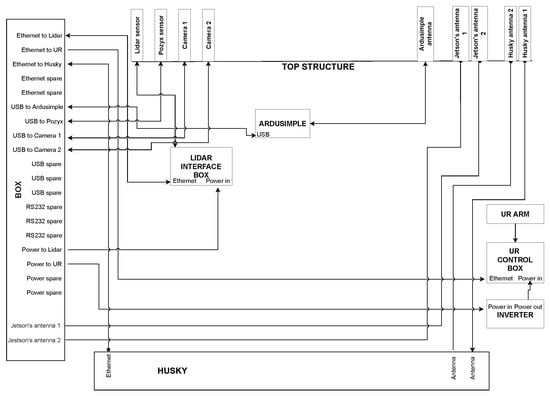
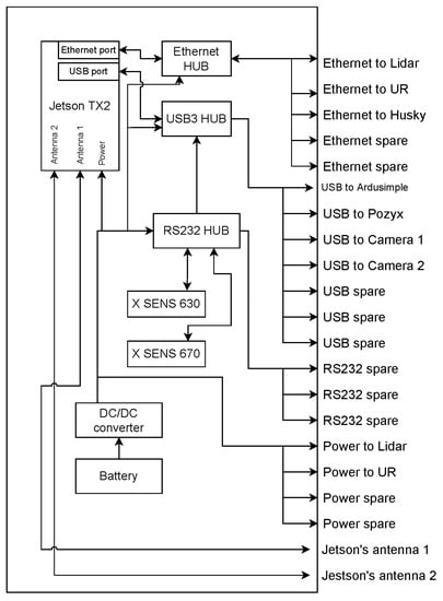
Figure 3.
Configuration of the electronics and of the high-level control box.
Once finalized, the mechanical and electronic systems used for our experiments were prototyped, as shown later in the experimental setup (see Section 3).
2.2. Configuration
In this work, a complete automatic navigation system with a multimodal sensor setup is conceived and implemented. The system consists of different software modules, including guidance, planning, perception, and main modules. Essential requirements for fully automatic operation of the robot in outdoor environments are mapping, a collision-free path-planning algorithm, path-following control, and detection and localization of obstacles. Each software module provides specific functions. i.e., the Guidance module was designed to control the mobile robot’s motion, the Planning module was developed to generate the shortest collision-free path, and the Perception module was created to detect and localize objects. We use as the central framework to implement a proposed automatic navigation system, and we developed packages to implement each software module. Coordination between software modules is illustrated in Figure 1 and Figure 4. In the following subsections, each coordinated system module, as well as the main block and developed algorithms, are explained in more detail.
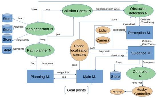
Figure 4.
The nodes scheme shows the system architecture in the first stage.
2.2.1. Main Module
The software modules are coordinated with each other through the Main module, the central module of the system. It receives user inputs, outputs commands, and calls upon other modules to perform a specific task. The main user input is the list of goals that the robot should visit. The goal points are expressed with respect to a pre-defined map of the environment that comes from previous knowledge of the environment. It can be made available as a grid-map of the orchard or, in future, thanks to the post-processing of a geo-referenced raster obtained through a previous survey with, e.g., a mapping drone. The grid-map of the environment is divided into a number of small square grid cells of the same size. Each grid cell can either correspond to a navigable area or to a space occupied by obstacles, e.g., trees.
The objective is to plan an optimal or sub-optimal route and then visit the goal points while avoiding obstacles, if needed. The Main module communicates with the Planning module to generate a path and with the Perception module to avoid obstacles. Given an initial pose and a sequence of goal points ( = , , …, ), the Planning module is then in charge of computing the shortest collision-free path connecting goal-to-goal points. Then, the Main module provides the reference waypoints to the Guidance module, which creates velocity commands to actuate the robot.
More in detail, as illustrated in Figure 4, the Main module receives a collision-free point-to-point path of waypoints between each pair of goal points from the Planning module, i.e., the Main module subscribes to the topic . Moreover, the Main module has information both on the map and on the proprioceptive sensor-related data, i.e., it subscribes to the topics and , which are computed according to the connected sensors, for localizing the robot on the map. It then sends the generated waypoints to the Guidance module to create a velocity command for the controller to move the robot towards the target point. The Perception module detects any unexpected obstacle, i.e., not present in the available map, that may appear along the path. For each newly detected object along the path, the Perception module evaluates whether it is occluding (blocking) the robot’s path or not. If the object blocks the path, it is considered an obstacle, and the cancels the planned path and waypoints. When this happens, the Main module receives an alert (through the ) and sends a request () to the Planning module to generate a new route considering the initial map updated with the obstacles, the robot’s current location as the initial pose, and the remaining goal points as locations to be visited. All the Store blocks represent the data-storage to handle different variables in different situations when needed, such as during the experimental tests.
2.2.2. Perception Module
The main purpose of the Perception module is to enable the robot to safely navigate through the environment while avoiding collisions with other objects. The Perception module can use the information either from a stereo RGB-D camera or LiDAR sensors to detect and localize objects around the robot that may eventually become obstacles. Both sensors provide point cloud data that must be filtered and processed to give an understanding of the surrounding environment. Since the two devices sense the environment differently, the provided point clouds have different properties. The LiDAR has a 360° view, whereas the camera is constrained to its horizontal field of view; the 3D LiDAR returns points in grayscale, while the camera can add red–green–blue (RGB) color information to the points. Therefore, to permit modularity and fast reconfiguration, two different packages for the two sensors have been developed. They share the same structure and class architecture.
The Perception module architecture is shown in Figure 5. There are two main nodes, called the Detector_node and BoundingBox_node, that are used to identify, localize, and estimate the size of possible obstacles. The Detector_node takes a point cloud as input and generates an array of point-cloud clusters as outputs. A filtered point cloud is used for debugging and visualization the scenario in Rviz, the 3D ROS visualizer. The BoundingBox_node takes as input the array of point-cloud clusters generated by the Detector_node and finds an axis-aligned bounding box for each cluster. The overall module can be decomposed into three main steps: pre-processing, clustering, and bounding-box definition.

Figure 5.
Perception module architecture.
The pre-processing step consists of a series of algorithms to prepare the data for the clustering step. Figure 6 presents an example of the perception module steps. Particularly, the point cloud is downsampled to reduce the computational load by using a voxel grid and pass-through filters (see Figure 6a) that mainly merge and approximate sets of points and cut the data to consider a reduced xyz-range of points. After downsampling the data, the Detector_node performs ground-removal using a plane-model segmentation algorithm [40] with a distance threshold parameter of 0.01 m. In the next step, since the ground is not perfect and the sensor is noisy, sometimes it happens that some points survive the segmentation step; an outlier-removal function is run to remove isolated points that remain after ground removal. Then, a DBSCAN algorithm [41] (see Figure 6b) is used to group all points belonging to the same object. A single point cloud is generated and added to an array for each object detected. The last step of the Perception module framework takes the array of clusters and finds an axis-aligned bounding box for each array element. When the system starts, the map frame is fixed in a known position in the environment and is used as the fixed-reference frame. We use this frame to generate axis-aligned bounding boxes for all the detected obstacles. When point cloud data is received from the sensor, it is filtered and the resulting point cloud is transformed with respect to the map frame. At that point, a bounding-box node generator to find the bounding boxes of the obstacles with coordinates expressed in the map frame (fixed frame) is run. The bounding box obtained is described with three coordinates representing the position of its center and three values representing the dimensions along coordinate axes. The final output of the perception module is published and accessible in the /BoundingBoxArray topic (/bbox in Figure 4).
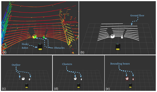
Figure 6.
Perception module steps: (a) raw PointCloud, (b) pass-through, (c) plane removal, (d) outlier removal and clustering, and (e) bounding-box generation.
2.2.3. Dynamic Map Implementation and Management
The definition and exploitation of the environmental map is fundamental for the implemented framework both for defining the goal points as well as for searching and finding the suitable path to be traveled. Suppose dynamic environments like the ones targeted in this research activity are considered. In that case, the map should be updated, and the path can be replanned if needed. The requirements for the map module can be defined as two sub-tasks.
The first one generates a dynamic map updated in real-time. The second sub-task checks if the computed path is still safely achievable (with no collisions) after the map is updated with the detected obstacle(s). The package developed to accomplish these tasks is called nav_map and consists of two nodes named MapGenerator_node and CollisionCheck_node. MapGenerator_node creates a first map of the known environment from a file as soon as the node starts setting its fixed frame in a know location, then it subscribes to the /BoundingBoxArray topic and updates the map every time a new message is received. Whenever a new message is received, it updates the map by removing or adding objects. The map is an OccupancyGrid map in which each cell can have three different values, respectively, it the cell represents a free area, obstacle area, or safety area. Besides the map, MapGenerator_node publishes an additional topic containing the coordinates of the cells containing an obstacle area. This information is used by CollisionCheck_node to check if the objects detected around the robot have to be considered as possible collision obstacles. CollisionCheck_node subscribes to the path topic /path and compares the obstacle’s cell coordinates and the path’s cell coordinates. If there is at least one overlap, CollisionCheck_node will trigger a collision message as true. This strategy was implemented to avoid that the robot considers as obstacles objects that are not in its path and so, avoiding planning a new path when the previously computed path is still valid and collision-free. An example is shown in Figure 7.
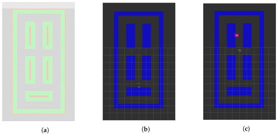
Figure 7.
Example of a known map provided in (a) csv, (b) OccupancyGrid free map, and (c) updated map with detected obstacles.
2.2.4. Planning Module
In the targeted applications, several given goal points that the robot needs to visit are fixed a priori, e.g., proximal monitoring of specific locations/plants. The Planning module based on is created to connect these goal points with the shortest collision-free path in the robot’s working environment. This module gets a request from the Main module to generate a path between two goal points (). The request is composed of the first goal point (current position of the robot) and the second goal point. The developed path-planning method, which we discuss in the following paragraph, is implemented to generate a collision-free path between every pair of sequenced goal points. For this purpose, a path planner node is created to compute a continuous obstacle-free path, where the path is assumed to go through a set of successive waypoints for k = 1, …, N; see Figure 4. This node gets the starting and end points (from ) as well as info from the map and the localization sensors and strategies adopted. Based on these data, the planner can generate waypoints representing a collision-free path between goal points. The Planning module is then in charge of sending the waypoints to the Guidance module. The path planner node is in charge of checking for the shortest path and waypoints from the robot’s current position to the goal position within the created map.
The path planner node uses an extended version of the authors’ developed path planning methods, called boundary-node method () and path enhancement method (PEM) [42,43,44]. The path-planning method calculates the shortest path considering obstacle avoidance to reach the destination point safely with the minimum distance traveled. The shortest path is generated in a two-step procedure. First, the Method generates the initial feasible path (IFP) between goal points. The IFP is generated from a sequence of waypoints w that the robot has to travel as it moves toward the destination point without colliding with obstacles.
An example of path planning and obstacle avoidance for a mobile robot in a static environment using is illustrated in Figure 8a. Based on the extended , the robot is simulated by a nine-node quadrilateral element. If the nodes are denoted by a vector , the robot’s location is represented by the centroid node , and nodes with represent the eight boundary nodes that help the robot move forward and avoid obstacles. The contour line represents the potential function utilized to direct the robot toward the goal point. It has the lowest potential value at the final destination point, and increases as the robot moves away. As shown in Figure 8a, the line color represents the potential value, i.e., red corresponds to the lowest potential value, and dark gray corresponds to the highest potential value. The sequence of the red circles represents the best solution to IFP. The simulated robot can only move in eight possible directions. In each iteration, the current location of the robot and boundary nodes move in one particular direction. Additionally, this method uses an optimization technique based on the lowest potential value to let the robot find the path and yield fast convergence. The node with the lowest potential value is chosen as the best position among all boundary nodes, and the robot updates its position to the best position.
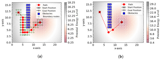
Figure 8.
Example of path planning for a mobile robot [44]: (a) The obtained solution to IFP by using , where the sequence of the red circles represents the IFP. (b) The shortest path found by using PEM, where the solid red line represents the shortest path.
The obtained IFP between goal points is not an optimal path in terms of total path length. Therefore, in the second step, the PEM is used to construct an optimal or near-optimal path from IFP by reducing the number of waypoints and the overall path length. Figure 8b illustrates the computed shortest path from waypoints. Waypoints defining the path are marked with red circles, while the red dashed line represents the shortest path. A more-detailed description of how the environment is created can be found in [43]. If the path provided by the path planner fails, or any unexpected obstacle is detected along the path, the path planner is contacted to compute a new path to the destination. This is the case when unexpected obstacles are detected in the working environment along the path. In this case, the path-planning method computes a new path for the robot to avoid collision with static and dynamic obstacles. Once the path is found, the Planning module forwards the waypoints to the Guidance module.
2.2.5. Guidance Module
This module aims to control the robot to follow the path, that consists of a series of waypoints joined by line segments. As reported in [45,46], the path-following method is one of the typical control methods for autonomous vehicles. This method allows a robot to follow a predefined path independent of time, and thus without any restriction on the time-propagation along the path. An accurate path-following method is an essential aspect of the automatic navigation of robots in farm environments.
This study employs and adapts a line-of-sight () guidance algorithm for path-following to drive the robot to follow a predefined path, which is based on a lookahead-based LOS guidance algorithm. The main advantages of lookahead LOS guidance are the simplicity and ease of implementation [46]. Furthermore, the lookahead method is used to compute control inputs in real-time, which is advantageous when the given path is not smooth or when the path is specified using waypoints [47]. The method assumes that the robot moves at a constant desired forward speed, and uses the relative pose (position and heading angle) between the robot and the nearest path segment being followed to generate the desired heading angle. Since the lookahead-based steering method only generates the desired speed and heading angle rather than the control inputs, it is known as a guidance law [48]. The lookahead approach utilizes motion information about the position, orientation, velocity, and acceleration.
In the following paragraph, we describe the robot motion model with only three degrees of freedom (). The robot’s motion is assumed to be constrained to the horizontal plane, and a plane view of the robot is shown in Figure 9. The three kinematic equations of the robot are reduced to [48]
where is the heading angle of the vehicle. We used the global reference frame G{x, y} and the body-coordinate frame B{xb, yb} to describe the robot’s motion, location, and orientation. As shown in Figure 9, the x axis of the global coordinate system G{x, y} points toward the North, the y axis points toward the East, and the z axis indicates downward. The body-fixed frame B{xb, yb} moves with the robot, the x axis points toward the head of the robot, the y axis points toward the right, the z axis indicates downward normal to the x–y surface, and U denotes the corresponding speed. The angle represents the slide-slip angle, and the angle represents the orientation angle of the mobile robot measured from the positive N axis of the body-fixed system. The point n denotes the center of the robot, which is a Cartesian coordinate about a global coordinate frame denoted by (, ). is the transformation matrix from B{xb, yb} to G{x, y}, which is given by
and
are the position and orientation (pose) vector and velocity vector (in body-fixed coordinates), respectively (see Figure 9). Here, the symbol is the Euclidean space of dimension n, S is an Euler angle defined on the interval , and is the Special Orthogonal Group of order 3 [48]. Thus, has three components representing two linear displacements and one angular rotation. The variables appearing in (3) include position , , orientation angle , surge speed u, sway speed v, and yaw rate r. In this study, we developed a speed controller using the kinematic model only. The force-controller we used was the native one of the Husky robot developed by the company. The development of a lower-level controller based on a dynamic model is left for future work and improvements.
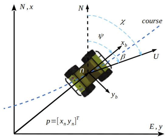
Figure 9.
Three-DOF maneuvering coordinate system definitions.
The overall path to be followed consists of a set of n straight-line segments connected by waypoints. The automatic controller is constructed to steer the vehicle along a time-independent path, for example the path between waypoints () and (). When the position of the robot is within a circle of acceptance with radius R around waypoint , so that
a switching mechanism is used to select the next waypoint . The waypoints are fed sequentially to have a smooth path without stop-and-go behavior.
- Line-of-Sight (LOS) guidance law:
Figure 9 and Figure 10 show the geometry of the LOS guidance problem and main variables. As shown in the figures, the position of the robot in global coordinates can be written as , and the corresponding speed is defined as
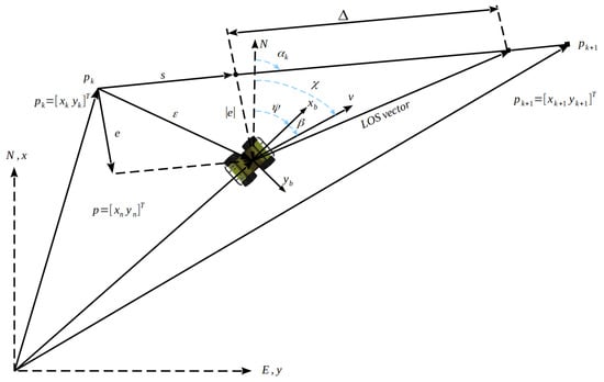
Figure 10.
Line-of-sight path-following definitions.
For an arbitrary waypoint on the path, the direction of the velocity vector with respect to the north axis is calculated by
As the robot starts following the path to move towards the goal point, it firstly rotates towards the first goal direction, and then the robot accurately passes through all waypoints between each pair of goal points. However, based on the path planner, the angle between waypoints is always less than 90 degrees [43]. Consider a straight-line path defined by two consecutive waypoints at positions and , respectively. The path makes an angle of
with respect to the north axis of the NED frame.
The coordinates of the robot in the path-fixed reference frame are
where is the transformation matrix from the inertial to the path-fixed frame given by
s is the along-track distance, and e is the cross-track error (see Figure 10). The cross-track error is defined as the orthogonal distance to the path tangential reference frame. From (8) and (9), the cross track error can be computed by
Its time derivative, which will be used later, is consequently given by
The control objectives are formulated to drive the cross-track error to zero by steering the robot and controlling its forward speed. With the lookahead-based steering method, a fixed parameter, known as the lookahead distance , which corresponds to a distance along the path ahead of point s, is used to define the LOS vector. The robot is steered so that its velocity vector is parallel to the LOS vector (Figure 10). The resulting velocity vector will have a component perpendicular to the path, driving the robot towards the path until the LOS vector is parallel to the path so that . Then, the Guidance module calculates the linear and angular velocities, which are sent to the Husky controller and afterward to wheel motors to let the robot move automatically between goal points. The Guidance module sends the linear and angular velocity inputs to move the Husky robot automatically inside the working environment.
3. Prototyping and Preliminary Experimental Tests
The conceived and designed layout has been implemented, and first navigation tests have been performed. The ground robot platform is mechanically designed to handle suitable sensors. Thus, the mechanical and electronic systems used for our experiments were prototyped and integrated on top of the main platform. The final configuration of the mobile robot for the first experimental tests is shown in Figure 11a,b. The second control box arrangement is reported in Figure 11c. The main ambient awareness sensors installed on the robot are a 3D LiDAR Velodyne VPL16 and an Intel Realsense D455 camera. The robot is equipped with a mini-ITX computer (see [36]), while the second control box embedded computer is a Jetson TX2 platform. The preliminary test targeted an emulated orchard and a safe navigation along a collision-free path given multiple goal points.
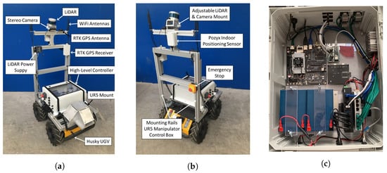
Figure 11.
Mechanical and electronic configuration of the experimental platform (UR5 manipulator not shown): (a) front view, (b) back view, and (c) second control box.
3.1. Emulated Scenario and Test Inputs
For the initial evaluation of the implemented framework, a lab-emulated orchard was created in which parallel rows of tree were considered fixed obstacles on the map. The experimental emulated scenario is shown in Figure 12a, and the Gazebo digital twin is shown in Figure 12b.
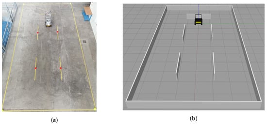
Figure 12.
Robot working environment: (a) the real environment; (b) the simulated environment using Gazebo.
The length and width of the environment are fixed to 13.2 m and 6.6 m, respectively. For simulating an orchard, the spacing between rows is set to 2.2 m (see [49]). The length of each row (static obstacles) is fixed at 2.2 m long. The robot’s working space is decomposed into rectangular grid cells, and each grid cell represents 10 cm in the robot’s working environment. The goal tolerance was set to 0.1 m, and the heading tolerance was set to 0.1 rad. The UGV chosen localization system was based on a filtered odometry approach; the Intel RealSense D455 -D camera or the Velodyne VLP-16 3D LiDAR were used (in different tests) for obstacle detection, and the extended was adopted for path planning. The vision system was set to operate in front of the robot, setting a view size of 5 × 6 × 1.5 m (xyz coordinates), and the obstacles were boxes of different dimension. The bounding boxes were generated with an offset of 0.2 m to ensure an additional safety. For path-tracking, the lookahead distance was set to 1 m for the LOS-guidance method, and the heading error was set to 0.05 rad.
Given the input data to define the goal points and the working environment, the map generator node creates a map. Afterward, the map data are processed with the goal points through the path planner to compute a collision-free path between each pair of goal points.
The planned path between each two goal points formed by a discrete sequence of poses, i.e., waypoints, is fed into the Guidance module. At the same time, the output of the Guidance module is mapped to the wheel motors by a simulated low-level controller running onboard.
3.2. Experimental Tests and Discussion
As per the envisioned tasks, the mobile robot was sent to the proper orchard locations to perform predefined tasks. Then, we experimentally tested the system to evaluate the automatic navigation performance in a generated given-map environment. In the first test configuration, we evaluated the automatic navigation performance of the robot under static environmental conditions. Then, in the second test configuration, we evaluated the robot’s navigation performance in a dynamic environment, i.e., with an unexpected obstacle along the path. During the experimental tests, we verified that the proposed framework generates an appropriate path, and the robot avoids static and dynamic obstacles without collisions.
Figure 13 and Figure 14 show the planned path for a mobile robot using in two testing scenarios as well as the performance of the navigation strategy in both testing scenarios. In the first test configuration (see Figure 13, the robot starts moving from initial position (0, 0) to visit three fixed goal points (, , and ) added to the pre-built map. The goal points were located at (−2.2, −2.2), (8.8, 2.2), and (4.5, −2.2). The red cells express the fixed obstacles, blue dashed lines represent the planned path of the robot, yellow circles in the figure define the goal points, and green cells represent the area related to the safety margin introduced to allow the robot to safely navigate and steer. In this study, we adopted a safety margin around obstacles to avoid the possibility of overlapping the paths traced by the robot overlapping with obstacles. As it can be appreciated in Figure 13a, the robot might move very close to the obstacle. Therefore, a certain safety margin for anti-collision has to be assured. Considering the robot dimensions and footprint, it has been defined with a constant-size of six grid cells. All fixed obstacles are given in parallel lines, and the goal points are given between obstacles. The robot localization sensors are utilized to determine where a mobile robot is located within the environment. In this test, a filtered-odometry, i.e., encoders and IMU, approach has been adopted. The current coordinates of the robot are compared with the predefined ranges of the fixed goal point, and if the robot is within the range, the coordinates of the next destination point are considered.
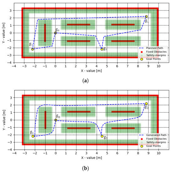
Figure 13.
Simulated environment with fixed obstacles: (a) planned path using ; (b) path executed by the robot.
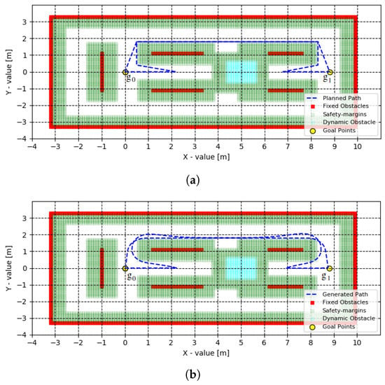
Figure 14.
Simulated environment with fixed and dynamic obstacles: (a) planned and replanned path using ; (b) path executed by the robot.
In the second scenario, the experimental test was carried out with the addition of a dynamic obstacle, as shown in Figure 14. The robot starts moving from the initial position (0, 0) to visit a fixed goal point () located at (8.8, 0.0), and then the robot returns to the initial point. Since the robot sensors detect a new obstacle that occludes the pre-planned path, the Planning module generates a new path from the current position to the destination point ().
The plots show that the robot’s executed path is coherent with the planned one. The mobile robot shows appropriate navigation accuracy and performs smooth motion along the environment with an average error ≤ 10 cm. The traveled path mostly depends on the robot’s kinematics, the accuracy of the sensors, and the environment. High navigation speeds lead to slightly higher errors. The proposed package always directs the robot to follow the planned path, and the robot moves close to the calculated path. The path starts from the robot’s initial position, passes through the intermediate goal points, and then returns to the initial point. A final path is assembled by connecting the paths between goal points in an iterative way until the path is completed, and the length of the path is the sum of the lengths of the goal-to-goal paths. From the first experimental scenario and reported experimental results, the generated path length is 24.3684 m, close to the 24 m of the ideal -planned path, thus showing good performance. Screenshots of the experimental tests at different locations are presented in Figure 15.
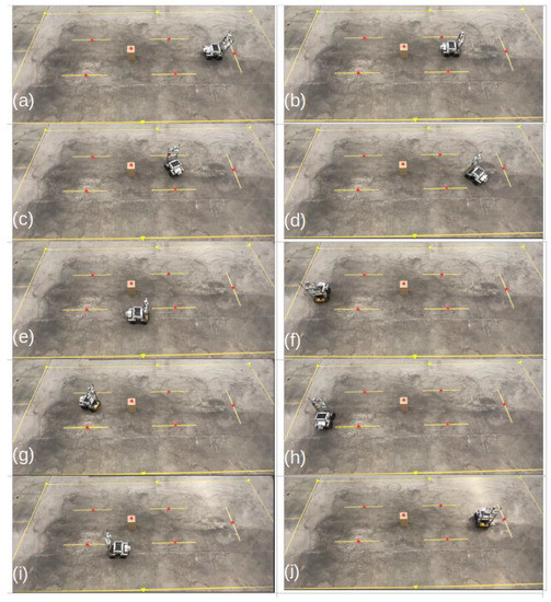
Figure 15.
From (a) start to (j) end: sequence of screenshots of the simulated orchard environment with obstacles (crop rows) showing the navigation test of the robot prototype in the physical environment, with the fixed obstacles represented by yellow lines, and the dynamic obstacle, not present in the predefined map, represented by the box.
Despite the overall good experimental results, the system may fail in certain circumstances. The perception module, for example, may fail detecting objects that have a size much smaller or much bigger than that of obstacles assumed during parameter tuning. This is due to the fact that when defining a cluster, the algorithm uses a min and max threshold value to constraint the number of points a cluster can contain. Additionally, because the planning module works based on the grid cells, increasing the cell size will reduce the system’s accuracy. In the same way, the guidance model may fail to control the robot if we set a very small value for the acceptance radius. In this scenario, due to the noisy data from the localization sensors, the robot may never reach the goal area, and thus it would not switch to the next goal point.
4. Conclusions
Here, the conceptual design and experimental implementation of a modular mobile robotic system for agricultural field tasks is presented. Based on the functional design concept and modules are conceived, developed and integrated on a Husky unmanned ground vehicle. In particular, the software modules are implemented using , following a high and low-level multi-layered approach, and allow the use of different sensors for localization and obstacle detection. Localization is implemented using a filtered-odometry method that can be integrated with indoor or outdoor positioning systems. Both an RGB-D camera and a 3D LiDAR sensor are configured for use on the platform, and either can be employed for obstacle avoidance. An extended Boundary Node Method, which has been specifically adapted for this work, is used for path planning. A modified Lookahead-based Line of Sight guidance algorithm is utilized for path following. Preliminary field tests in an emulated orchard scenario demonstrate that the system can perform path-following with a suitable accuracy, and obstacle detection, with path re-planning when needed. Planned future work will include intensive experimental testing, detailed data analyses, as well as performance assessments of the system’s capabilities of executing the three scenarios (monitoring, harvesting, and spraying) in both emulated and real environments.
Author Contributions
Conceptualization and methodology, R.A.S., G.T., K.D.v.E. and R.V.; software, validation, and formal analysis, R.A.S. and G.T.; resources, K.D.v.E. and R.V.; writing—original draft preparation, R.A.S., G.T. and R.V.; writing—review and editing, all; supervision, G.C., K.D.v.E. and R.V.; project administration and funding acquisition, K.D.v.E. and R.V. All authors have read and agreed to the published version of the manuscript.
Funding
This research was supported in part by the “Reconfigurable Collaborative Agri-Robots (RECOARO)” Südtirol/Alto Adige 4th Call (project #4122) and by the European Regional Development Fund (ERDF), FiRST Lab Project #FESR1084.
Institutional Review Board Statement
Not applicable.
Informed Consent Statement
Not applicable.
Data Availability Statement
Not applicable.
Acknowledgments
The authors are grateful to Matteo Malavasi, who designed and fabricated some of the electronic systems of the robot, and Josef Zelger, who designed and fabricated the mechanical superstructure.
Conflicts of Interest
The authors declare no conflict of interest.
References
- Mondejar, M.E.; Avtar, R.; Diaz, H.L.B.; Dubey, R.K.; Esteban, J.; Gómez-Morales, A.; Hallam, B.; Mbungu, N.T.; Okolo, C.C.; Prasad, K.A.; et al. Digitalization to achieve sustainable development goals: Steps towards a Smart Green Planet. Sci. Total Environ. 2021, 794, 148539. [Google Scholar] [CrossRef] [PubMed]
- Nasirahmadi, A.; Hensel, O. Toward the Next Generation of Digitalization in Agriculture Based on Digital Twin Paradigm. Sensors 2022, 22, 498. [Google Scholar] [CrossRef]
- Monteiro, A.; Santos, S.; Gonçalves, P. Precision agriculture for crop and livestock farming—Brief review. Animals 2021, 11, 2345. [Google Scholar] [CrossRef]
- Shafi, U.; Mumtaz, R.; García-Nieto, J.; Hassan, S.A.; Zaidi, S.A.R.; Iqbal, N. Precision agriculture techniques and practices: From considerations to applications. Sensors 2019, 19, 3796. [Google Scholar] [CrossRef] [PubMed]
- Department, I.S. World Robotics 2021—Service Robots; VDMA Services GmbH: Frankfurt am Main, Germany, 2021. [Google Scholar]
- Blender, T.; Buchner, T.; Fernandez, B.; Pichlmaier, B.; Schlegel, C. Managing a mobile agricultural robot swarm for a seeding task. In Proceedings of the IECON 2016-42nd Annual Conference of the IEEE Industrial Electronics Society, Florence, Italy, 23–26 October 2016; pp. 6879–6886. [Google Scholar]
- Oberti, R.; Marchi, M.; Tirelli, P.; Calcante, A.; Iriti, M.; Tona, E.; Hočevar, M.; Baur, J.; Pfaff, J.; Schütz, C.; et al. Selective spraying of grapevines for disease control using a modular agricultural robot. Biosyst. Eng. 2016, 146, 203–215. [Google Scholar] [CrossRef]
- Maini, P.; Gonultas, B.M.; Isler, V. Online coverage planning for an autonomous weed mowing robot with curvature constraints. IEEE Robot. Autom. Lett. 2022, 7, 5445–5452. [Google Scholar] [CrossRef]
- McAllister, W.; Osipychev, D.; Davis, A.; Chowdhary, G. Agbots: Weeding a field with a team of autonomous robots. Comput. Electron. Agric. 2019, 163, 104827. [Google Scholar] [CrossRef]
- Quan, L.; Jiang, W.; Li, H.; Li, H.; Wang, Q.; Chen, L. Intelligent intra-row robotic weeding system combining deep learning technology with a targeted weeding mode. Biosyst. Eng. 2022, 216, 13–31. [Google Scholar] [CrossRef]
- Tinoco, V.; Silva, M.F.; Santos, F.N.; Rocha, L.F.; Magalhães, S.; Santos, L.C. A review of pruning and harvesting manipulators. In Proceedings of the 2021 IEEE International Conference on Autonomous Robot Systems and Competitions (ICARSC), Santa Maria da Feira, Portugal, 28–29 April 2021; pp. 155–160. [Google Scholar]
- Botterill, T.; Paulin, S.; Green, R.; Williams, S.; Lin, J.; Saxton, V.; Mills, S.; Chen, X.; Corbett-Davies, S. A Robot System for Pruning Grape Vines. J. Field Robot. 2017, 34, 1100–1122. [Google Scholar] [CrossRef]
- Kim, W.S.; Lee, D.H.; Kim, Y.J.; Kim, T.; Lee, W.S.; Choi, C.H. Stereo-vision-based crop height estimation for agricultural robots. Comput. Electron. Agric. 2021, 181, 105937. [Google Scholar] [CrossRef]
- Vidoni, R.; Gallo, R.; Ristorto, G.; Carabin, G.; Mazzetto, F.; Scalera, L.; Gasparetto, A. Byelab: An agricultural mobile robot prototype for proximal sensing and precision farming. In Proceedings of the ASME International Mechanical Engineering Congress and Exposition, Proceedings (IMECE), Tampa, FL, USA, 3–9 November 2017; Volume 4A. [Google Scholar] [CrossRef]
- Quaglia, G.; Visconte, C.; Scimmi, L.; Melchiorre, M.; Cavallone, P.; Pastorelli, S. Design of a UGV powered by solar energy for precision agriculture. Robotics 2020, 9, 13. [Google Scholar] [CrossRef]
- Bac, C.W.; Van Henten, E.J.; Hemming, J.; Edan, Y. Harvesting robots for high-value crops: State-of-the-art review and challenges ahead. J. Field Robot. 2014, 31, 888–911. [Google Scholar] [CrossRef]
- Moysiadis, V.; Sarigiannidis, P.; Vitsas, V.; Khelifi, A. Smart farming in Europe. Comput. Sci. Rev. 2021, 39, 100345. [Google Scholar] [CrossRef]
- Oliveira, L.; Moreira, A.; Silva, M. Advances in agriculture robotics: A state-of-the-art review and challenges ahead. Robotics 2021, 10, 52. [Google Scholar] [CrossRef]
- Kumar, A.; Deepak, R.S.; Kusuma, D.S.; Sreekanth, D. Review on multipurpose agriculture robot. Int. J. Res. Appl. Sci. Eng. Technol. 2020, 8, 1314–1318. [Google Scholar] [CrossRef]
- Sowjanya, K.D.; Sindhu, R.; Parijatham, M.; Srikanth, K.; Bhargav, P. Multipurpose autonomous agricultural robot. In Proceedings of the 2017 International Conference of Electronics, Communication and Aerospace Technology (ICECA), Coimbatore, India, 20–22 April 2017; Volume 2, pp. 696–699. [Google Scholar]
- Nandeesh, T.; M Kalpana, H. Smart Multipurpose Agricultural Robot. In Proceedings of the CONECCT 2021: 7th IEEE International Conference on Electronics, Computing and Communication Technologies, Bangalore, India, 9–11 July 2021. [Google Scholar] [CrossRef]
- Tauze Zohora Saima, F.; Tamanna Tabassum, M.; Islam Talukder, T.; Hassan, F.; Sarkar, P.K.; Howlader, S. Advanced Solar Powered Multipurpose Agricultural Robot. In Proceedings of the 2022 3rd International Conference for Emerging Technology, INCET, Belgaum, India, 27–29 May 2022. [Google Scholar] [CrossRef]
- Levin, M.; Degani, A. A conceptual framework and optimization for a task-based modular harvesting manipulator. Comput. Electron. Agric. 2019, 166, 104987. [Google Scholar] [CrossRef]
- Le, A.V.; Arunmozhi, M.; Veerajagadheswar, P.; Ku, P.C.; Minh, T.H.Q.; Sivanantham, V.; Mohan, R.E. Complete path planning for a tetris-inspired self-reconfigurable robot by the genetic algorithm of the traveling salesman problem. Electronics 2018, 7, 344. [Google Scholar] [CrossRef]
- Grimstad, L.; From, P.J. Thorvald II-a modular and re-configurable agricultural robot. IFAC-PapersOnLine 2017, 50, 4588–4593. [Google Scholar] [CrossRef]
- Levin, M.; Degani, A. Design of a Task-Based Modular Re-Configurable Agricultural Robot. IFAC-PapersOnLine 2016, 49, 184–189. [Google Scholar] [CrossRef]
- Denis, D.; Thuilot, B.; Lenain, R. Online adaptive observer for rollover avoidance of reconfigurable agricultural vehicles. Comput. Electron. Agric. 2016, 126, 32–43. [Google Scholar] [CrossRef]
- Youchun, Z.; Gongyong, Z. Design of Multimodal Neural Network Control System for Mechanically Driven Reconfigurable Robot. Comput. Intell. Neurosci. 2022, 2022, 2447263. [Google Scholar] [CrossRef] [PubMed]
- Xu, R.; Li, C. A modular agricultural robotic system (MARS) for precision farming: Concept and implementation. J. Field Robot. 2022, 39, 387–409. [Google Scholar] [CrossRef]
- Lytridis, C.; Kaburlasos, V.G.; Pachidis, T.; Manios, M.; Vrochidou, E.; Kalampokas, T.; Chatzistamatis, S. An Overview of Cooperative Robotics in Agriculture. Agronomy 2021, 11, 1818. [Google Scholar] [CrossRef]
- GARotics. Green Asparagus Harvesting Robotic System. Available online: http://echord.eu/garotics (accessed on 27 July 2022).
- Albani, D.; IJsselmuiden, J.; Haken, R.; Trianni, V. Monitoring and mapping with robot swarms for agricultural applications. In Proceedings of the 2017 14th IEEE International Conference on Advanced Video and Signal Based Surveillance (AVSS), Lecce, Italy, 29 August–1 September 2017; pp. 1–6. [Google Scholar]
- Reisch, B.I.; Owens, C.L.; Cousins, P.S. Grape. In Fruit Breeding; Springer: Berlin/Heidelberg, Germany, 2012; pp. 225–262. [Google Scholar]
- Fernandez, R.; Montes, H.; Surdilovic, J.; Surdilovic, D.; Gonzalez-De-Santos, P.; Armada, M. Automatic detection of field-grown cucumbers for robotic harvesting. IEEE Access 2018, 6, 35512–35527. [Google Scholar] [CrossRef]
- FiRST-Lab. Field Robotics South-Tyrol Lab. Available online: https://firstlab.projects.unibz.it/ (accessed on 24 July 2022).
- Robotics, C. Husky Technical Specifications. Available online: https://www.clearpathrobotics.com/husky-unmanned-ground-vehicle-robot/ (accessed on 24 July 2022).
- Universal Robots. Available online: https://www.universal-robots.com/ (accessed on 31 August 2022).
- ArduSimple. Available online: https://www.ardusimple.com/ (accessed on 31 August 2022).
- Pozyx. Available online: https://www.pozyx.io/ (accessed on 31 August 2022).
- Fischler, M.A.; Bolles, R.C. Random sample consensus: A paradigm for model fitting with applications to image analysis and automated cartography. Commun. ACM 1981, 24, 381–395. [Google Scholar] [CrossRef]
- Ester, M.; Kriegel, H.P.; Sander, J.; Xu, X. A density-based algorithm for discovering clusters in large spatial databases with noise. In Proceedings of the KDD, Portland, OR, USA, 2–4 August 1996; Volume 96, pp. 226–231. [Google Scholar]
- Saeed, R.; Reforgiato Recupero, D.; Remagnino, P. The boundary node method for multi-robot multi-goal path planning problems. Expert Syst. 2021, 38, e12691. [Google Scholar] [CrossRef]
- Saeed, R.; Recupero, D.; Remagnino, P. A Boundary Node Method for path planning of mobile robots. Robot. Auton. Syst. 2020, 123, 103320. [Google Scholar] [CrossRef]
- Saeed, R.; Recupero, D. Path planning of a mobile robot in grid space using boundary node method. In Proceedings of the ICINCO 2019—16th International Conference on Informatics in Control, Automation and Robotics, Prague, Czech Republic, 29–31 July 2019; Volume 2, pp. 159–166. [Google Scholar] [CrossRef]
- Lekkas, A.M.; Fossen, T.I. A time-varying lookahead distance guidance law for path following. IFAC Proc. Vol. 2012, 45, 398–403. [Google Scholar] [CrossRef]
- Wang, X.; Wu, G. Modified LOS path following strategy of a portable modular AUV based on lateral movement. J. Mar. Sci. Eng. 2020, 8, 683. [Google Scholar] [CrossRef]
- Ahn, J.; Shin, S.; Kim, M.; Park, J. Accurate Path Tracking by Adjusting Look-Ahead Point in Pure Pursuit Method. Int. J. Automot. Technol. 2021, 22, 119–129. [Google Scholar] [CrossRef]
- von Ellenrieder, K.; Licht, S.; Belotti, R.; Henninger, H. Shared human–robot path following control of an unmanned ground vehicle. Mechatronics 2022, 83, 102750. [Google Scholar] [CrossRef]
- Du, F.; Deng, W.; Yang, M.; Wang, H.; Mao, R.; Shao, J.; Fan, J.; Chen, Y.; Fu, Y.; Li, C.; et al. Protecting grapevines from rainfall in rainy conditions reduces disease severity and enhances profitability. Crop Prot. 2015, 67, 261–268. [Google Scholar] [CrossRef]
Publisher’s Note: MDPI stays neutral with regard to jurisdictional claims in published maps and institutional affiliations. |
© 2022 by the authors. Licensee MDPI, Basel, Switzerland. This article is an open access article distributed under the terms and conditions of the Creative Commons Attribution (CC BY) license (https://creativecommons.org/licenses/by/4.0/).