Abstract
Fault diagnosis of bearing with small data samples is always a research hotspot in the field of bearing fault diagnosis. To solve the problem, a convolutional block attention module (CBAM)-based attentional feature fusion with an inception module based on a capsule network (Capsnet) is proposed in the paper. Firstly, the original vibration signal is decomposed into multiple intrinsic mode function (IMF) sub-signals by the ensemble empirical mode decomposition (EEMD), and then the original vibration signal and the corresponding former four order IMF sub-signals are input into the inception modules to extract the features. Secondly, these features are concatenated and optimized by the CBAM. Finally, the selected sensitive features are fed into the Capsnet to diagnose the faults. Through the multifaceted experiment analysis on fault diagnosis of bearing with small data samples, the diagnosis results demonstrate that the proposed attentional feature fusion with inception based on Capsnet not only diagnoses the fault of bearing with small data samples, but also is superior to other feature fusion methods, such as feature fusion with inception based on Capsnet and attentional feature fusion with inception based on CNN, etc., and other single diagnosis models such as Capsnet with CBAM and inception, and CNN with CBAM and inception.
1. Introduction
A bearing is a very important part of a rotating machine, whose failure can not only cause the shutdown of the whole mechanical equipment, but also result in serious economic losses for a factory. In order to ensure the safety of mechanical equipment, it is necessary to monitor and diagnose the bearing faults. Nowadays, deep learning is widely applied to the field of fault diagnosis, because of automatic extraction features from the raw vibration signal without manual favors and end-to-end diagnosis ability. Many deep learning models have been developed to diagnose the bearing fault effectively, such as deep belief network (DBN), convolution neural network (CNN), and long short-term memory network (LSTM). In the process of fault diagnosis, these deep learning models need sufficient data samples [1,2,3,4,5]. However, in the real industrial scenario the number of faulty data samples is much lower, and so small data sample fault diagnosis based on deep learning has become a research focus [6].
Small data sample fault diagnosis means that the small data samples, less than 30 generally in industrial practice, are used to train the deep learning model to diagnose the bearing faults. However, the deep learning models are prone to overfit because of the small data samples, which leads to low diagnosis accuracy. Currently, many variants of deep learning are being developed to diagnose the fault of bearings using few data samples. Generative adversarial network (GAN) and other data augmentation methods, i.e., over sampling and its variants, are suggested to create additional valid samples for training deep learning models [7]. In addition, transfer learning is also utilized to exploit deep learning models trained in source domain, where enough fault data samples are available to improve the diagnosis accuracy based on limited data samples in the target domain [8]. Obviously, these data augmentation methods can diagnose the faults with small samples effectively by generating substantial high-quality samples based on the distribution of real samples or applying emerging transfer learning technologies. However, these methods are often unable to fully learn the various effective features of the limited samples, because of the loss of the diversity of these generated data samples and relatively small data samples in the target domain. In other words, although the data augmentation method increases the number of data samples, the generated data samples cannot cover the data distribution of all fault data samples, which can lead to limited diagnosis accuracy improvement.
Feature-based methods are also utilized to solve the problem of small sample fault diagnosis, and these models can learn the fault-related features to diagnose the bearing fault. CNN is widely applied in the field of fault diagnosis because of the strong ability of the extraction features. The design of big convolution kernels is beneficial in enhancing the robustness of features [9], while that of small convolution kernels effectively extracts abstract features. Furthermore, time-step information can be ignored and some fault information can be concealed in vibration signals.
In order to capture more fault-related features, feature fusion methods are often used to overcome the limitation of small data samples to achieve high diagnosis accuracy and generalization because of the mutual complementation among different feature information, which can make use of all complementary features extracted from different signals to solve the diagnosis difficulty of small data samples [10,11]. Some feature fusion methods combined with CNN are proposed to diagnose bearing faults. Duy used CNN to fuse features extracted from a time–frequency plot of three sensor signals to obtain a reliable and highly accurate diagnosis, even though these sensor signals contain strong noise [12], while Xia et al. fed multiple vibration signals to CNN to achieve the diagnosis results with higher accuracy and robustness [13]. Considering the nonstationarity of vibration signal, and the limitations of local extraction features of CNN, Han et al. used the different frequency band sub-signals decomposed by the wavelet transform method as the input of a dynamic ensemble CNN to diagnose the bearing faults effectively [14]. Li et al. utilized the global time domain statistical features and local features extracted by CNN as the input of an ensemble CNN to diagnose the fault with high accuracy and robustness [15]. Although these feature fusion methods based on CNN can improve the diagnosis accuracy and generalization, some features concealed in the vibration signal cannot be thoroughly dug out, which can affect the performance of diagnosis models.
Time–frequency analysis methods are often used to decompose the original vibration signal into different frequency sub-signals to depict the fault-related information from different scales, such as short-time Fourier transform (STFT), wavelet transform (WT), and empirical mode decomposition (EMD). Owing to the nonstationary characteristic of a vibration signal, an ensemble empirical mode decomposition (EEMD) is used to decompose the signal into different intrinsic mode function (IMF) sub-signals here. Considering that increasing the number of convolutional layers can lead to the over-fitting and network gradient vanishing or dispersion, an inception module with different convolution kernels is utilized to extract more features from the different IMF signals [16]. Furthermore, for better diagnostic analysis, these extracted features are fused to depict the fault-related information. However, it is well-known that redundant or irrelevant features can reduce the diagnosis accuracy of a diagnosis model. Attention mechanisms can focus on the sensitive features and suppress those unimportant features [17]. To improve the diagnosis accuracy and generalization, an attention mechanism based on a convolutional block attention module (CBAM) [18] is adopted to select some fault-sensitive features.
However, these features extracted by CNN are all scalars, which cannot depict the relative position relationship between features, resulting in the loss of the fault-related information. A capsule network (Capsnet) can extract feature vector, which can realize the spatial information coding of bearing healthy states, while the vector’s modulus and direction can represent the probability and the attitude information of fault features. Owing to these merits, some information fusion methods based on Capsnet are proposed to diagnose a fault using small samples. For example, Capsnet combined with the Bi-LSTM and CNN is applied to the fault diagnosis of a bearing with few fault data samples [19]; a multisensory data fusion method based on ensemble Capsnet is used to diagnose bearing faults with high accuracy and robustness [20]; and a novel Capsnet combined with wide convolution and multi-scale convolution is also proposed to effectively diagnose bearing faults with small data samples [21].
As mentioned above, small data sample fault diagnosis is always difficult because of the small fault data samples in industry practice. Although some data augmentation methods can resolve the problem to a certain extent, the diagnosis accuracy still needs to be improved further because of the loss of the sample diversity of these generated data samples. The features, especially the intrinsic fault features, can use the fault-related information to effectively diagnose the fault without considering the number of data samples. How to obtain more sensitive fault features is the key to the small data samples fault diagnosis. Therefore, a novel attentional feature fusion method with an inception module based on Capsnet is proposed to diagnose the small sample fault of bearings in this paper. The main contribution of the proposed diagnosis method are summarized as follows:
- (1)
- A feature fusion method based on Capsnet is proposed to diagnose the fault of bearings with small data samples with high accuracy and generalization, which combines all fused features extracted from IMF sub-signals with Capsnet;
- (2)
- The inception module is used to extract the features from the different IMF sub-signals decomposed by EEMD, which can use different convolution kernel sizes to capture more features from the different scales;
- (3)
- The CBAM is utilized to select fault-sensitive features from all fused features to improve the diagnosis accuracy and generalization of the Capsnet.
The remainder sections are organized as follows. The proposed attentional feature fusion method with inception module based on Capsnet is described in Section 2; Section 3 provides the fault diagnosis analysis of bearings with small data samples. Finally, the conclusions are summarized in Section 4.
2. The Proposed Attentional Feature Fusion with Inception Based on Capsnet
In order to solve the accuracy and generalization of small data sample fault diagnosis, a novel attentional feature fusion with inception based on Capsnet, which can capture more sensitive fault features, is proposed and the corresponding diagnosis flowchart is shown in Figure 1. The original vibration signal is truncated by the sliding time window and divided into n data segments; the data segment is decomposed into different IMF sub-signals by the EEMD method; and the inception module is utilized to extract different features from the different IMF sub-signals and original date segment. After that, these features fused by the concatenation method are optimized by the CBAM module. At last, the selected sensitive features are input into Capsnet to diagnose the fault of the bearing with small data samples.
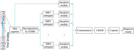
Figure 1.
Diagnosis flowchart of attentional feature fusion with inception based on Capsnet.
2.1. EEMD
In order to obtain more fault-related information concealed in the original vibration signal, EEMD, which is the improved version of EMD, is used to decompose the original vibration into different IMF sub-signals and solve the problem of mode mixing in the EMD method by a noise-assisted analysis method [22]. It produces a collection of series by adding the white noise with the statistical property of uniform distribution in the frequency range of the primitive signal firstly, and then processes the newly acquired sequences with the EMD method. The algorithm is briefly described as follows:
- (1)
- When the Gaussian white noise sequence with the given amplitude is added to the original vibration data segment x(t), the new ith signal sequence can be obtained, where is the added white noise of the ith trial;
- (2)
- Use EMD to decompose the time sequence , then the jth IMF components and one residual component are obtained as the following formulae:where is the jth IMF component of n IMF components of the ith trial;
- (3)
- Repeat the step (1) and step (2) with the given M trials, and the ensemble mean of all trials can be calculated. The corresponding formulae are written as follows:
- (4)
- The decomposition result of the original data segment x(t) by the EEMD can be obtained by the following equation:where r(t) is the final residual component of EEMD.
Thereinto, the amplitude of the added white noise and the number M of trials play an important role in the decomposition process. In addition, considering the amount of fault information in IMF sub-signals and the computational complexity, the former four order IMF sub-signals are selected by the cross-correlation coefficient between each IMF sub-signal and original vibration signals of each fault class, which is depicted in detail in this reference [23].
2.2. Inception Module
Generally, CNN can use a convolution layer to extract features from the IMF sub-signals decomposed from original vibration signal by the EEMD and original vibration signal. The size of convolution kernels determines the range of the receptive field. The larger the convolution kernel size is, the more information the extracted feature parameters contain.
In order to obtain multi-view fault-related information, and avoid overfitting and network gradient vanishing or dispersion, the inception block parallels convolutional layers with convolution kernels of different sizes, which is used to extract the features from different scales. The structure of the inception v1 module that is used to extract the features from the IMF sub-signal or original vibration signal is shown in Figure 2. The inception v1 module contains four parallel convolution layers with different kernel sizes. The first three parallel convolution layers consist of different convolution layers with kernel size 1 × 1, 3 × 3, and 5 × 5, respectively, to extract features from different scales, while the last parallel convolution layer consists of a max-pooling layer with kernel size 3 × 3 and a convolution layer with kernel size 1 × 1. Therefore, the convolution layer with kernel size 1 × 1 can reduce the computation complexity and the number of channels in every parallel convolution layer, and the max-pooling layer with kernel size 3 × 3 can reduce the computation complexity of the model. After the computation of four parallel convolution layers, output feature maps of each parallel layer are concatenated to form new feature maps with more channel dimensions.
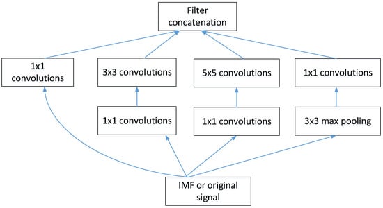
Figure 2.
The structure of inception v1 module.
2.3. Convolutional Block Attention Module (CBAM)
It is well-known that sensitive fault features can improve the accuracy of a diagnosis model. In order to obtain some sensitive features, CBAM, which can focus on channel and spatial information at the same time, is adopted to select the discriminative features [19]; its structure, which consists of a channel attention process and a spatial attention process, is displayed in Figure 3. The input features are fed into two attention modules to obtain the refined feature; the features selection process of these attention modules, i.e., the channel attention module and spatial attention module, are represented, respectively, by the two following equations.
where is the attention weight in the channel dimension; is the attention weight in spatial dimension, which is the spatial attention map obtained in the spatial attention module by the selection of sensitive features of the channel; F′ represents the input feature map F multiplying the channel attention map; and F″ represents the result of the spatial attention map multiplying F′, which is the output refined features of the CBAM module. The symbol ⊗ denotes element-wise multiplication. Reference [18] provides the detailed algorithm of CBAM.

Figure 3.
The structure of the CBAM attention mechanism.
2.4. Capsule Network (Capsnet)
Capsnet replaces a group of scalar neurons of CNN with a group of vector neurons, the output vector length of which normalize to the interval of [0,1], which can preserve the pose information for the object to reduce the information loss by the extracted feature vector. As shown in Figure 4, the architecture of Capsnet, which consists of the convolution layer with ReLU activation layer, the primary capsule layer, and the digital capsule layer, contains convolutional operation and dynamic routing agreement.
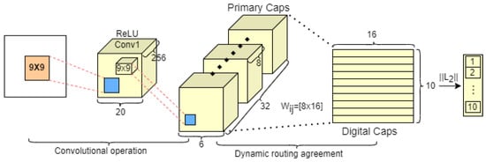
Figure 4.
The basic architecture of Capsnet.
The convolution layer with the ReLU layer and primary capsules layer is convolutional operation layer, which can transform the raw input data into primary capsules. For a given , the convolution layer with ReLU layer can be described by the following equation,
where the notation indicates convolution operator, and are weights and biases, is a nonlinear activation function ReLU, and are output nonlinear representations.
Afterwards, the primary capsule layer, taking the former representations as inputs, is regarded as a convolutional layer, which is followed by a reshaping operation and a nonlinearity transformation. After the convolutional calculation, the primary convolutional representations are reshaped into a new primary convolutional with different dimensions, which indicates the number of primary capsules with the n dimension vector in the primary capsule layer. The nonlinear transformation is performed by a nonlinear squashing function, which can transform the output vector length of capsule into an interval of [0,1], whose length denotes the probability that the presence of the category is presented by the capsules, but the direction of the vector does not change. The computation process is called a dynamic routing algorithm based on the agreement, which can be used to build the complex nonlinear map relationship between the primary capsule layers and digital capsule layers.
The length of the activity vector of each digital capsule presents the presence probabilities of an instance for each category, which is equivalent to the categories to be classified. The operation process of the dynamic routing algorithm is shown in Figure 5. Given are the neurons in the primary capsule layer, the weighted sum of all the middle prediction vectors from the capsules in the primary capsule layer is the total input to a digit capsule. The is obtained by multiplying the neuron in the primary capsule layer with a transformation matrix , which is described as:
the input is calculated by the following formula:
the output vector is obtained by the squashing function map of :
where j denotes the jth output neuron of the digital capsule, and is coupling coefficients updated by the dynamic routing algorithm in the training stage, which is denoted by the routing softmax function:
where is the log prior probabilities of the coupling coefficient that the capsule i couples with the capsule j, which is updated by the following equation:
where the “agreement” is defined as follows:
Thus, with the iterations from (6) to (12), all these parameters are determined.

Figure 5.
The dynamic routing algorithm in capsule network.
2.5. Diagnosis Algorithm of Attentional Feature Fusion with Inception Based on Capsnet
The diagnosis algorithm of the proposed attentional feature fusion with inception based on Capsnet is illustrated in Figure 6, and the detailed calculation processes are depicted as follows:
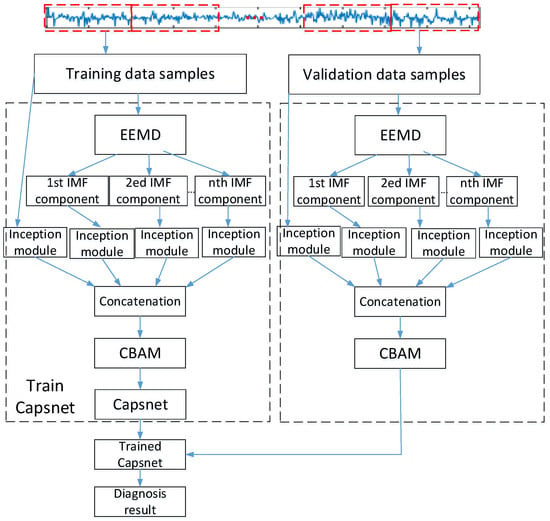
Figure 6.
The diagnosis process of feature fusion based on Capsnet.
- (1)
- The original vibration signals of the bearing are segmented by the sliding time window. These data segmentations are divided into training data samples and validation data samples;
- (2)
- These training and validation data samples are decomposed into different IMF sub-signals;
- (3)
- The IMF sub-signals and original data sample are fed into the inception module for extracting the features. Following this, the former four order IMF sub-signals are selected;
- (4)
- All these extracted features are concatenated to be optimized by the CBAM module, and then these sensitive features are selected;
- (5)
- The sensitive features are used to train the Capsnet, and then the trained Capsnet can be obtained. After that, the sensitive features of the validation samples are fed to the trained Capsnet to obtain the final diagnosis results.
In the training process of Capsnet, the margin loss function , depicted as Equation (15), is adopted,
where is the indicator function; if class k is present, otherwise 0; k denotes the fault class; is the upper bound to punish false positives; is the lower bound to punish false negative; λ is the coefficient; and the value of the parameters m+, m−, and λ are set as 0.9, 0.1, and 0.5, respectively. is the probability value of the fault class k, which cannot be less than 0.9, generally, if the fault class k is present. Otherwise, it cannot be greater than 0.1 if the fault class k is not present.
3. Fault Diagnosis of Rolling Bearing with Few Samples
To verify the validity and generalization of the proposed feature fusion with inception based on Capsnet, the collected vibration signal originated from a dataset of rolling element bearings [24]. The test rig of the bearing fault is displayed in Figure 7, which is composed of a high-speed spindle, steel base plate, rigid support, and precision sledge. The body of the high-speed spindle, driving the rotation of a shaft, is fixed to the rigid support, which rests on a massive steel base plate; the same plate carries a couple of supports (positions B1 and B3) for the outer rings of two identical roller bearings, while the inner rings of these bearings are connected to a very short and tick hollow shaft (Figure 7c). The outer ring of bearing B2 is linked to a precision sledge, whose motion is orthogonal to the shaft; when the sledge is pulled through the rotation of a nut, two parallel springs (green in Figure 7a) are compressed and produce the required load. The acceleration sensors are mounted at position A1, and in the data acquisition system, the sampling rate of vibration signal is 51.2 K/s.
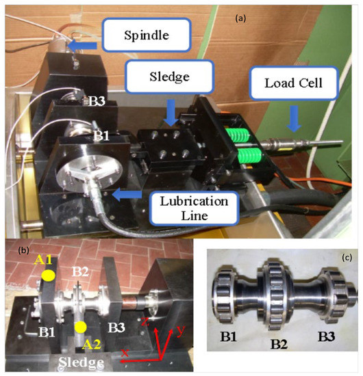
Figure 7.
The experimental test rig: (a) general view of the test rig; (b) positions of the two accelerometers and the reference coordinate system; (c) the shaft with its three roller bearings [24].
To simulate the different fault categories of bearing, the single point defects (defect diameter is 0.45 mm) are introduced into the inner race and outer race. The test speed is 6000 rpm, and the load is 0, 1006 N, and 992 N. The y-axial (vertical coordinates of point A1) vibration signal is used for the diagnosis analysis of bearing faults. Table 1 shows the detailed data samples statistics. Four different datasets with a different number of training samples are listed and referred to as datasets A/B/C/D, respectively; the data sample number of each fault category is 5, 10, 15, and 20 in each dataset, the total number of training samples is 15, 30, 45, and 60, respectively, and the total number of validation samples in these datasets is150 in each dataset. Additionally, the length of the sliding time window, which is used to segment the vibration signal, is 1024; namely, each data sample has 1024 sample points, and the adjacent data samples have no overlapping region.

Table 1.
The training/validation data statistics of rolling bearing.
3.1. Diagnosis Analysis
According to the diagnosis flowchart of the proposed attentional feature fusion with inception based on Capsnet, dataset A is decomposed into different IMF sub-signals, and the former four order IMF sub-signals are selected for the fault diagnosis of the bearing, because of the larger cross-correlation coefficient between the IMF sub-signal and original signal of each fault category, which are shown in the Table 2. Figure 8 shows the corresponding original normal vibration signal and former four order IMF sub-signals. From Figure 8, it can be seen that the former four order IMF sub-signals mainly contain high frequency and medium frequency components, which can depict the dynamic characters from different scales.

Table 2.
Cross-correlation coefficient between IMF sub-signal and original signal of each fault.
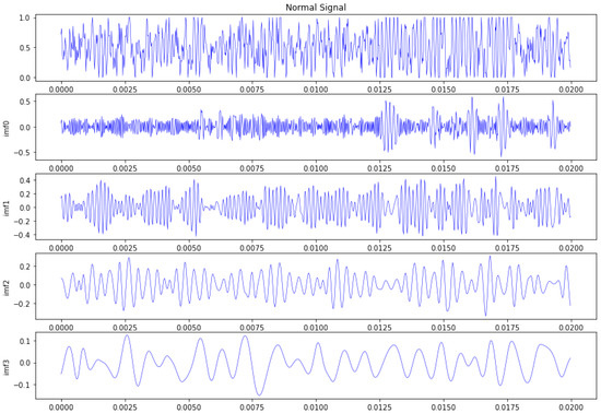
Figure 8.
The normal vibration signal and the former four order IMF sub-signals.
After that, the original data sample and the former four order IMF sub-signals are reshaped into the maps of 1 × 32 × 32 size to feed into the inception module for extracting the features, and all the features are fused by the concatenation operator to constitute multi-channel feature maps. Then, the sensitive features selected by the CBAM module are reshaped and input into Capsnet to diagnose the bearing faults. Figure 9 shows the diagnosis accuracy and cross entropy of training dataset B and the validation dataset. Table 3 provides the validation accuracy using different datasets to train Capsnet. From Table 3, it can be seen that the validation accuracy of the four datasets all achieve 1. This demonstrates that the proposed attentional feature fusion method with an inception module based on Capsnet can effectively diagnose the bearing fault with small data samples.
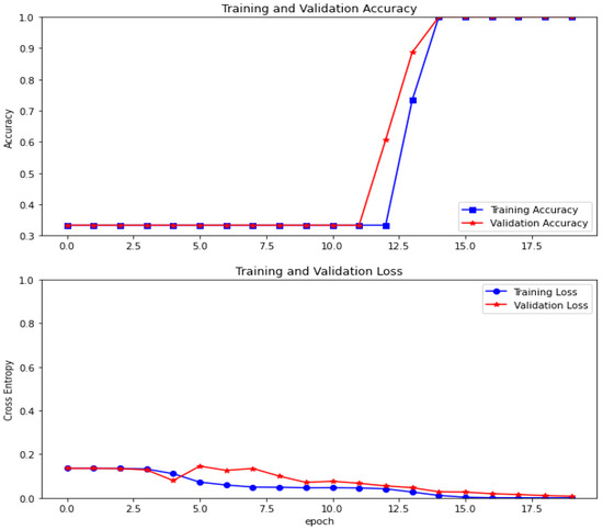
Figure 9.
The accuracy and loss of training dataset and validation dataset.

Table 3.
The validation accuracy using different training datasets.
3.2. Comparison with Other Diagnosis Methods
In order to verify the superiority of the proposed attentional features fusion with inception based on Capsnet, comparisons to the diagnosis accuracy of other methods, namely, attentional features fusion without inception based on Capsnet, features fusion with inception based on Capsnet, features fusion without inception based on Capsnet, attentional features fusion with inception based on CNN, feature fusion without inception based on CNN, single Capsnet with CBAM and inception, single Capsnet without CBAM and inception, single CNN with CBAM and inception, and single CNN without CBAM and inception are implemented on the four datasets. The diagnosis results are shown in the Table 4 and Figure 10. From Table 4 and Figure 10, it can be seen that the diagnosis accuracy of the attentional feature fusion (with CBAM) with inception based on Capsnet is the highest among all the ten diagnosis methods, which are all higher than that of attentional feature fusion without inception (with Conv layer of 128 @ 2 × 2 kernel size) based on Capsnet. This indicates that the inception module extract more features from different scales, which depicts fault information about the bearing. The accuracy of the attentional feature fusion with inception based on Capsnet is higher than that of feature fusion (without CBAM) with inception based on Capsnet. This signifies that the CBAM module selects the sensitive features to improve the accuracy of the diagnosis model. The accuracy of the feature fusion with inception based on Capsnet is higher than that of the feature fusion without inception based on Capsnet; this also demonstrate that the inception module further improves the diagnosis accuracy. This demonstrates that the CBAM and inception module improve the diagnosis accuracy of a diagnosis method.

Table 4.
Diagnosis accuracy of different methods using different training datasets.
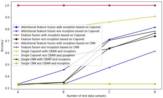
Figure 10.
The diagnosis accuracy of different diagnosis methods on four datasets.
In addition, Table 4 and Figure 10 show that the diagnosis accuracy of the attentional feature fusion with inception based on CNN (with a Conv layer of 128 @ 2 × 2 kernel size and an average pooling layer of 2 × 2 size, a flatten layer, two dense layers, and softmax activation) and the accuracy of the attentional feature fusion with inception based on Capsnet all achieve 1 in the four datasets. This indicates that the feature fusion with inception and CBAM improves the diagnosis accuracy of CNN and Capsnet. The accuracy of feature fusion without inception based on CNN for the four datasets is 0.333, 0.333, 0.474, and 0.612, respectively, which are also all lower than that of the feature fusion without inception based on Capsnet. They are all lower than that of the attentional feature fusion with inception based on Capsnet and that of the attentional feature fusion with inception based on CNN. This indicates that the feature fusion without inception based on Capsnet is superior to the feature fusion without inception based on CNN, and that the CBAM and inception module improve the accuracy of a diagnosis model.
Furthermore, Table 4 and Figure 10 also show that the accuracy of single Capsnet without CBAM and inception and accuracy of single CNN without CBAM and inception is0.333 for all four datasets, which is the lowest among these ten diagnosis methods. This also demonstrates that the CBAM selects sensitive feature to improve the diagnosis accuracy. The accuracy of single Capsnet (with Conv layer of 128 @ 2 × 2 kernel size and original vibration signal) with CBAM and inception is 0.747, 0.813, 0.86, and 0.907 for the four datasets, respectively, which is higher than that of single CNN (with a Conv layer of 128 @ 2 × 2 kernel size and an average pooling layer of 2 × 2 size, a flatten layer, two dense layers, softmax activation, and original signal) with CBAM and inception. It is also higher than that of attentional feature fusion without inception based on Capsnet and that of attentional feature fusion without inception based on CNN. This is because the inception module also extracts more features from the original data sample. This also shows that the inception module greatly improves the diagnosis accuracy of a diagnosis model, which can produce a better diagnosis performance than that of the feature fusion without inception. The single Capsnet with CBAM and inception is superior to the single CNN with CBAM and inception, and this is because the feature vector extracted by Capsnet captures more fault formation.
In order to verify the superiority of the proposed attentional features fusion with inception based on Capsnet further, comparisons to diagnosis accuracy of data augmentation methods such as single CNN with an over-sampling method and single Capsnet with over-sampling (the number of data samples for each fault class is 50) are also implemented. Table 5 provides the comparison results using four different datasets. From Table 5, it can be seen that the diagnosis accuracy of the proposed attentional feature fusion with inception based on Capsnet is the highest among these three methods on the four datasets, and the accuracy of the single Capsnet with over-sampling is higher than that of the single CNN with over-sampling. Furthermore, from Table 4 and Table 5, it can be also seen that the accuracy of single CNN with over-sampling is higher than that of single CNN with CBAM and inception, and the accuracy of single Capsnet with over-sampling is higher than that of single Capsnet with CBAM and inception. This demonstrates that over-sampling can improve the diagnosis accuracy of single CNN and single Capsnet with small data samples, but the proposed attentional features fusion with inception based on Capsnet is more effective in solving the problem of small sample fault diagnosis. This is mainly because the proposed method can extract some sensitive fault features.

Table 5.
Comparison with other data augmentation using different training datasets.
All these discussions demonstrate that the feature fusion with inception can capture more fault features from different scales about the bearing, which can collect complementary fault information because of small data samples, and the CBAM module can select the sensitive features. Thus, the attentional feature fusion with inception based on Capsnet achieves high diagnosis accuracy on small data samples, and has a better diagnosis performance than other diagnosis methods on small data samples.
3.3. Generalization Analysis Using Noisy Dataset
In order to verify the generalization and superiority of the proposed attentional feature fusion with inception based on Capsnet, the different SNR dataset B, contaminated by white noise of different intensities, is utilized. Table 6 and Figure 11 provide the diagnosis accuracy of four feature fusion diagnosis models such as attentional feature fusion with inception based on Capsnet, attentional feature fusion without inception based on Capsnet, feature fusion with inception based on Capsnet, and feature fusion without inception based on Capsnet. From Table 6 and Figure 11, it can be seen that the attentional feature fusion with inception based on Capsnet effectively diagnoses the small samples faults on five different SNR training datasets. When the SNR is −20 db, −10 db, −1 db, 10 db, and 20 db, the diagnosis accuracy of the attentional feature fusion with inception based on Capsnet is 1 on these five different SNR datasets, and the highest among the four diagnosis models. The accuracy of the attentional feature fusion without inception based on Capsnet for the five datasets is 0.333, 0.333, 0.333, 0.384, and 0.428, respectively, which is lower than that of attentional feature fusion with inception based on Capsnet and higher than that of the feature fusion with inception based on Capsnet and that of the feature fusion without inception based on Capsnet. This also indicates that the inception module can capture more feature information on the bearing fault, which improves the diagnosis accuracy of the feature fusion without inception based on Capsnet, and the CBAM module can select the sensitive features to improve the diagnosis accuracy of the feature fusion with inception based on Capsnet further. All these demonstrate that CBAM and the inception module improve the diagnosis accuracy and generalization of the feature fusion method based on Capsnet.

Table 6.
The diagnosis accuracy of four feature fusion diagnosis models on different SNR datasets.
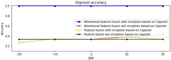
Figure 11.
Diagnosis accuracy of four different feature fusion methods on different SNR datasets.
4. Conclusions
In order to solve the difficulty of diagnosing bearings with small fault data samples, a novel attentional feature fusion with inception based on Capsnet is proposed in this paper. The original vibration signal and the corresponding multiple IMF sub-signals decomposed by the EEMD method are input into multiple inception modules to extract the features, and then these features are concatenated and optimized by the CBAM module. Finally, these sensitive features are fed into Capsnet to diagnose the bearing faults.
To verify the diagnosis effectiveness and generalization of the proposed attentional feature fusion with inception based on Capsnet, a multifaceted comparison of attentional feature fusion without inception based on Capsnet; feature fusion with inception based on Capsnet; feature fusion without inception based on Capsnet; attentional feature fusion with inception based on CNN; feature fusion without inception based on CNN; single Capsnet with CBAM and inception; single Capsnet without CBAM and inception; single CNN with CBAM and inception and single CNN without CBAM and inception is performed on four different small fault datasets, and one of these datasets with five different SNR. These diagnosis results demonstrate that the proposed attentional feature fusion with inception based on Capsnet can achieve excellent diagnosis accuracy and generalization on these small fault data samples and small noisy data samples, and it is superior to the other nine diagnosis models for the diagnosis of bearings with few fault data samples. All these show that the proposed attentional feature fusion with inception based on Capsnet has a wide application prospect in the field of machinery fault diagnosis with small data samples.
Author Contributions
Conceptualization, Z.X.; methodology, Y.W. and Z.X.; software, Y.W. and Z.X.; validation, Z.X. and Z.W.; formal analysis, Y.W.; investigation, Y.W. and Z.X.; data curation, Y.W.; writing—original draft preparation, Y.W. and Z.X.; writing—review and editing, Z.X.; visualization, Y.W.; supervision, W.X. and Z.W.; project administration, Z.X.; funding acquisition, Z.X. All authors have read and agreed to the published version of the manuscript.
Funding
This research was funded by the National Natural Science Foundation of China (Grant No. 51775391), the Open Research Foundation of State Key Lab. of Digital Manufacturing Equipment and Technology in Huazhong University of Science and Technology (Grant No. DMETK F2017010).
Institutional Review Board Statement
No applicable.
Informed Consent Statement
No applicable.
Data Availability Statement
The data that were used to support this study are available at the Politecnico di Torino rolling bearing test rig [24].
Conflicts of Interest
The authors declare no conflict of interest.
References
- Li, J.; Li, X.; He, D.; Qu, Y. Unsupervised rotating machinery fault diagnosis method based on integrated SAE–DBN and a binary processor. J. Intell. Manuf. 2020, 31, 1899–1916. [Google Scholar] [CrossRef]
- Wang, Z.; Dong, Y.; Liu, W.; Ma, Z. A Novel Fault Diagnosis Approach for Chillers Based on 1-D Convolutional Neural Network and Gated Recurrent Unit. Sensors 2020, 20, 2458. [Google Scholar] [CrossRef]
- Wang, X.; Mao, D.; Li, X. Bearing fault diagnosis based on vibro-acoustic data fusion and 1D-CNN network. Measurement 2021, 173, 108518. [Google Scholar] [CrossRef]
- Huang, D.; Fu, Y.; Qin, N.; Gao, S. Fault diagnosis of high-speed train bogie based on LSTM neural network. Sci. China Inf. Sci. 2021, 64, 119203. [Google Scholar] [CrossRef]
- Zhang, J.; Jiang, Y.; Luo, H.; Yin, S. Prediction of material removal rate in chemical mechanical polishing via residual convolutional neural network. Control. Eng. Pract. 2021, 107, 104673. [Google Scholar] [CrossRef]
- Zhang, X.; He, C.; Lu, Y.; Chen, B.; Zhu, L.; Zhang, L. Fault diagnosis for small samples based on attention mechanism. Measurement 2022, 187, 110242. [Google Scholar] [CrossRef]
- Li, X.; Zhang, W.; Ding, Q.; Sun, J.Q. Intelligent rotating machinery fault diagnosis based on deep learning using data augmentation. J. Intell. Manuf. 2020, 31, 433–452. [Google Scholar] [CrossRef]
- Wu, J.; Zhao, Z.; Sun, C.; Yan, R.; Chen, X. Few-shot transfer learning for intelligent fault diagnosis of machine. Measurement 2020, 166, 108202. [Google Scholar] [CrossRef]
- Zhang, W.; Peng, G.; Li, C.; Chen, Y.; Zhang, Z. A New Deep Learning Model for Fault Diagnosis with Good Anti-Noise and Domain Adaptation Ability on Raw Vibration Signals. Sensors 2017, 17, 425. [Google Scholar] [CrossRef]
- Osamor, V.C.; Okezie, A.F. Enhancing the weighted voting ensemble algorithm for tuberculosis predictive diagnosis. Sci. Rep. 2021, 11, 14806. [Google Scholar] [CrossRef]
- Ma, G.; Yang, X.; Zhang, B.; Shi, Z. Multi-feature fusion deep networks. Neurocomputing 2016, 218, 164–171. [Google Scholar] [CrossRef]
- Hoang, D.T.; Tran, X.T.; Van, M.; Kang, H.J. A Deep Neural Network-Based Feature Fusion for Bearing Fault Diagnosis. Sensors 2021, 21, 244. [Google Scholar] [CrossRef] [PubMed]
- Xia, M.; Li, T.; Xu, L.; Liu, L.; De Silva, C.W. Fault diagnosis for rotating machinery using multiple sensors and convolutional neural networks. IEEE/ASME Trans. Mechatron. 2017, 99, 101–110. [Google Scholar] [CrossRef]
- Yan, H.; Tang, B.; Lei, D. Multi-level wavelet packet fusion in dynamic ensemble convolutional neural network for fault diagnosis. Measurement 2018, 127, 246–255. [Google Scholar]
- Li, H.; Huang, J.; Ji, S. Bearing Fault Diagnosis with a Feature Fusion Method Based on an Ensemble Convolutional Neural Network and Deep Neural Network. Sensors 2019, 19, 2034. [Google Scholar] [CrossRef] [PubMed]
- Li, X.; Kong, X.; Zhang, J.; Hu, Z.; Shi, C. A study on fault diagnosis of bearing pitting under different speed condition based on an improved inception capsule network. Measurement 2021, 181, 109656. [Google Scholar] [CrossRef]
- Zhang, J.; Jiang, Y.; Wu, S.; Li, X.; Luo, H.; Yin, S. Prediction of remaining useful life based on bidirectional gated recurrent unit with temporal self-attention mechanism. Reliab. Eng. Syst. Saf. 2022, 221, 108297. [Google Scholar] [CrossRef]
- Woo, S.; Park, J.; Lee, J.Y.; Kweon, I.S. CBAM: Convolutional block attention module. arXiv 2018, arXiv:1807.06521. [Google Scholar]
- Han, T.; Ma, R.; Zheng, J. Combination bidirectional long short-term memory and capsule network for rotating machinery fault diagnosis. Measurement 2021, 176, 109208. [Google Scholar] [CrossRef]
- Huang, R.; Li, J.; Li, W.; Cui, L. Deep Ensemble Capsule Network for Intelligent Compound Fault Diagnosis Using Multisensory Data. IEEE Trans. Instrum. Meas. 2020, 69, 2304–2314. [Google Scholar] [CrossRef]
- Wang, Y.; Ning, D.; Feng, S. A Novel Capsule Network Based on Wide Convolution and Multi-Scale Convolution for Fault Diagnosis. Appl. Sci. 2020, 10, 3659. [Google Scholar] [CrossRef]
- Mohd Jaafar, N.S.; Aziz, I.A.; Jaafar, J.; Mahmood, A.K. An Approach of Filtering to Select IMFs of EEMD in Signal Processing for Acoustic Emission [AE] Sensors. In Intelligent Systems in Cybernetics and Automation Control Theory, CoMeSySo 2018; Advances in Intelligent Systems and Computing; Silhavy, R., Silhavy, P., Prokopova, Z., Eds.; Springer: Cham, Switzerland, 2019; Volume 860. [Google Scholar]
- Mingliang, L.; Bing, L.; Jianfeng, Z.; Keqi, W. An application of ensemble empirical mode decomposition and correlation dimension for the HV circuit breaker diagnosis. J. Control. Meas. Electron. Comput. Commun. 2019, 60, 105–112. [Google Scholar]
- Daga, A.P.; Fasana, A.; Marchesiello, S.; Garibaldi, L. The Politecnico di Torino rolling bearing test rig: Description and analysis of open access data. Mech. Syst. Signal Process. 2019, 120, 252–273. [Google Scholar] [CrossRef]
Publisher’s Note: MDPI stays neutral with regard to jurisdictional claims in published maps and institutional affiliations. |
© 2022 by the authors. Licensee MDPI, Basel, Switzerland. This article is an open access article distributed under the terms and conditions of the Creative Commons Attribution (CC BY) license (https://creativecommons.org/licenses/by/4.0/).