Optimized Trapezoidal Acceleration Profiles for Minimum Settling Time of the Load Velocity

Abstract

This paper deals with a method for generating symmetrical trapezoidal acceleration profiles for the motor of a vibrating system in rest-to-velocity motion. The aim was to significantly reduce the acceleration time and residual load vibration of lightly damped systems. Under undamped conditions, the analytical values of the jerk time are found to be in relation to the estimated natural frequency and the minimum value of the acceleration time is provided, also taking into account a limit value for motor acceleration. The analysis of the sensitive curves allows the designer to understand the magnitude of the residual vibration generated by an incorrect estimate of the natural frequency. Numerical simulations, with a closed-chain controlled motor and a zero or very small structural damping coefficient of the oscillating system, confirm the validity of the proposed method.

1. Introduction

Oscillating systems are often found in machines in which a motor is controlled by means of a closed chain with co-located actuation and measurement and a load is connected to the motor through an equivalent compliant shaft. The mechanical system can be modelled with two modes: a rigid mode and a vibrating one.

Examples range from flexible robots to pick-and-place machines, cranes, micromachines, satellites, etc. Productivity demands require a reduction in the load motion time. This means minimizing its settling time, evaluated from the start of the motor motion.

The rationale is to minimize the sum of the motion time of the motor reference and the subsequent free vibrations of the load, which must be strongly attenuated or even suppressed as a consequence of the motor motion profile.

In addition to solutions based on mechanical system modification or feedback control, there is the command shaping [1], which is a profiling technique of the motor command through adequate algorithms based on system dynamics. Compared with feedback control, command shaping does not require sensors for measurements and acts preemptively, without the delay caused by a closed chain. However, it includes a delay with respect to the specified motion time. Obviously, the designer of the motion profile must have some information about the natural frequency of the load oscillations, but often with a margin of uncertainty. Furthermore, excepting the fact that it is much less than one, the dimensionless structural damping coefficient of the load oscillations is more often than not unknown. Therefore, one of the main problems of command shaping is that it must be robust with respect to these uncertainties.

The technical literature in this regard is very extensive. A review of papers concerning the dynamic analysis of flexible manipulators was presented by Dwivedy and Eberhard in [2], and another concerning the command shaping technique by Singhose in [3]. Other more recent papers presented the application of command shaping techniques to robots, cranes, satellites, dielectric elastomer actuators, etc., optimizing them with artificial intelligence, combining them with feedback control, applying them to multi-mode and non-linear systems, and taking into account initial and final conditions that are different from zero, etc. Rashidifar et al. [4] used genetic algorithms to optimize a command shaping technique for a single link of a flexible robot. Huang et al. [5] studied the dynamics of double-pendulum cranes with distributed-mass beams, in which the system parameters have a large effect on the second mode natural frequency, and applied robust command smoothing at the input to suppress the payload oscillations. Kotake et al. [6] suppressed the residual vibrations of a hoisting load by applying appropriate feed-forward acceleration to the trolley; the solution works within a natural period with small swing angles, and within longer times with large ones. Alghanim et al. [7] optimized the generation of discrete time-shaped acceleration profiles that eliminate payload oscillations during simultaneous travel and hoisting maneuvers and show robust performance. Mar et al. [8] considered a double pendulum and applied a combined input shaping and feedback control, which allows fast point-to-point motion and effective attenuation of the external disturbance effect, while also being robust with respect to model uncertainties. Fujioka and Singhose [9] controlled a non-linear double-pendulum by developing an optimized input-shaped model reference control based on a single-pendulum. They used a Ljapunov control law referred to the first mode and optimized the controller parameters to minimize the motion time in the presence of different constraints. Maghsoudi et al. [10] considered a non-linear gantry crane with a variable cable length and reduced vibrations by using a command shaper with distributed delay. Ichikawa et al. [11] studied a command shaper applied to the control of a quadrotor to reduce the oscillations of a suspended payload. Hou et al. [12] designed a shaped reference angular acceleration to reduce residual vibration at the end of flexible satellites maneuvers. Sharma [13] developed a command shaper to attenuate vibration of an electro-statically driven dielectric elastomer actuator when it is subject to a multi-step input signal. Newmann et al. [14] studied a neural network to predict the pose-dependent natural frequency of a robot and used it in conjunction with a command shaping technique to attenuate vibration. Alhazza et al. [15] modified a smooth waveform command shaper to improve its behavior in a point-to-point motion with non-zero initial and final conditions.

Other papers modified the command input to attenuate undesired vibrations. Hoshyari et al. [16] investigated a method for retargeting artist-specified inputs on the motors of physical flexible robot characters to minimize unwanted structural vibrations while respecting the artist’s intention. Shah et al. [17] optimized the input voltage waveform of a piezoelectric inkjet printhead by introducing, after a first pulse for jetting, a second pulse to attenuate residual vibrations of the actuating membrane.

Other works are closer to the approach of the present paper. Ha et al. [18] minimized the residual vibrations induced by different types of trapezoidal acceleration profiles by applying a pole-zero cancellation technique that shows robustness against the modeling errors. Yoon et al. [19] applied trapezoidal velocity profiles in a point-to-point motion, whose acceleration and deceleration time must contain an integer number of natural periods to suppress residual vibrations. Meckl and Arestides [20] applied a torque input and optimized trapezoidal acceleration profiles to obtain the minimum motion time of the load with an acceleration limit of the motor.

This paper deals with a rest-to-velocity motion, but it is also preparatory to another paper concerning a point-to-point motion. It considers symmetrical trapezoidal acceleration profiles (STAP) as input. Even today, STAPs are widely used in both rest-to-velocity and point-to-point motions. Moreover, in many industrial control systems a STAP is the only acceleration profile that the operator can implement. The STAPs have the advantage of simplicity and offer the possibility of reducing load vibration in a system with an oscillating dof. The acceleration time $t_a$ and the two jerk times $t_j$, corresponding to the two oblique sides of the trapezoid, must be chosen appropriately to achieve the minimum load settling time, evaluated from the start of the motion.

As mentioned above, the settling time of the load is the sum of two parts: the acceleration time $t_a$ of the motor reference and the subsequent time taken by the residual vibrations of the load to abate. The proposed solution is sub-optimal, since the latter time is estimated on the base of the sensitivity curve (SC), i.e., of the amplitude of the residual velocity oscillation without any damping, with respect to the steady-state value, when the actual natural frequency is different from the estimated one. This SC of velocity is similar to that of position described in [1,3].

This work draws inspiration from [20]; however, compared with it, the input is not a torque command, but the motor acceleration. Moreover, the field of investigation is enlarged to acceleration times $t_a$ that are greater than twice the minimum possible value $t_{a,min}$ due to the acceleration limit ${\ddot{\vartheta }}_{Max}$ of the motor, and thus to STAPs that cannot reach this acceleration. The acceleration limit ${\ddot{\vartheta }}_{Max}$ is also discussed, taking into account the oscillations of motor torque and load acceleration. Furthermore, the dimensionless analysis was performed with reference to the acceleration time $t_a$ and not to $t_{a,min}$. This allows the designer to have an analytical formula that expresses the jerk time as a function of the natural frequency for the conditions of zero residual vibration of the load. In addition, the limits set on the acceleration time $t_a$ by the natural frequency $f_n$ of the oscillating system were investigated. Finally, the analysis of the SCs allows the designer to judge the machine from the point of view of the residual vibration of the load velocity when the natural frequency is different from the estimated one.

Specifically, in this paper, Section 2.1 deals with the system model. Section 2.2 analyzes the acceleration profile of the motor in relation to $t_{a,min}$, while Section 2.3 investigates the zero residual vibrations conditions of the load. Section 2.4 analyzes the SCs, which show the maximum residual velocity oscillation when the natural frequency is different from the estimated one. Section 3 discusses the results using various examples, and Section 4 provides guidelines for designing the STAP once the specifications are given. Finally, Section 5 presents the conclusions.

2. Materials and Methods

This section is divided into four sub-sections. In the first, the model of the oscillating system is presented and the corresponding equations are obtained in both the time and Laplace domains. In the second, the general characteristics of a STAP for a rest-to-velocity motion of the motor are studied, taking into account the acceleration limit of the motor. In the third, the residual vibration suppression is achieved by equating the exciting term, evaluated at the undamped natural frequency of the system, to zero. This allows the designer to obtain analytical expressions of the jerk time as a function of the estimated natural frequency. In the fourth, the SCs are considered, taking into account an inaccurate estimate of the natural frequency and the dimensionless damping coefficient.

2.1. System Model

The oscillating system is shown in Figure 1. The motor, whose moment of inertia is $J_M$, moves the load, whose moment of inertia is $J_L$, through a compliant shaft. The shaft inertia is negligible, its torsional stiffness is k and its structural damping coefficient is c. The equivalent viscous resistance inside the motor is neglected. The motor torque is $M_m$ and its absolute value has a maximum $M_{M,max}$ due to the electronic driver feeding the motor.

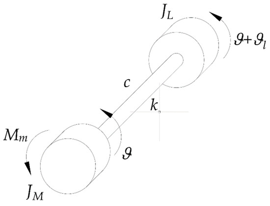
Figure 1. Model of the oscillating system.

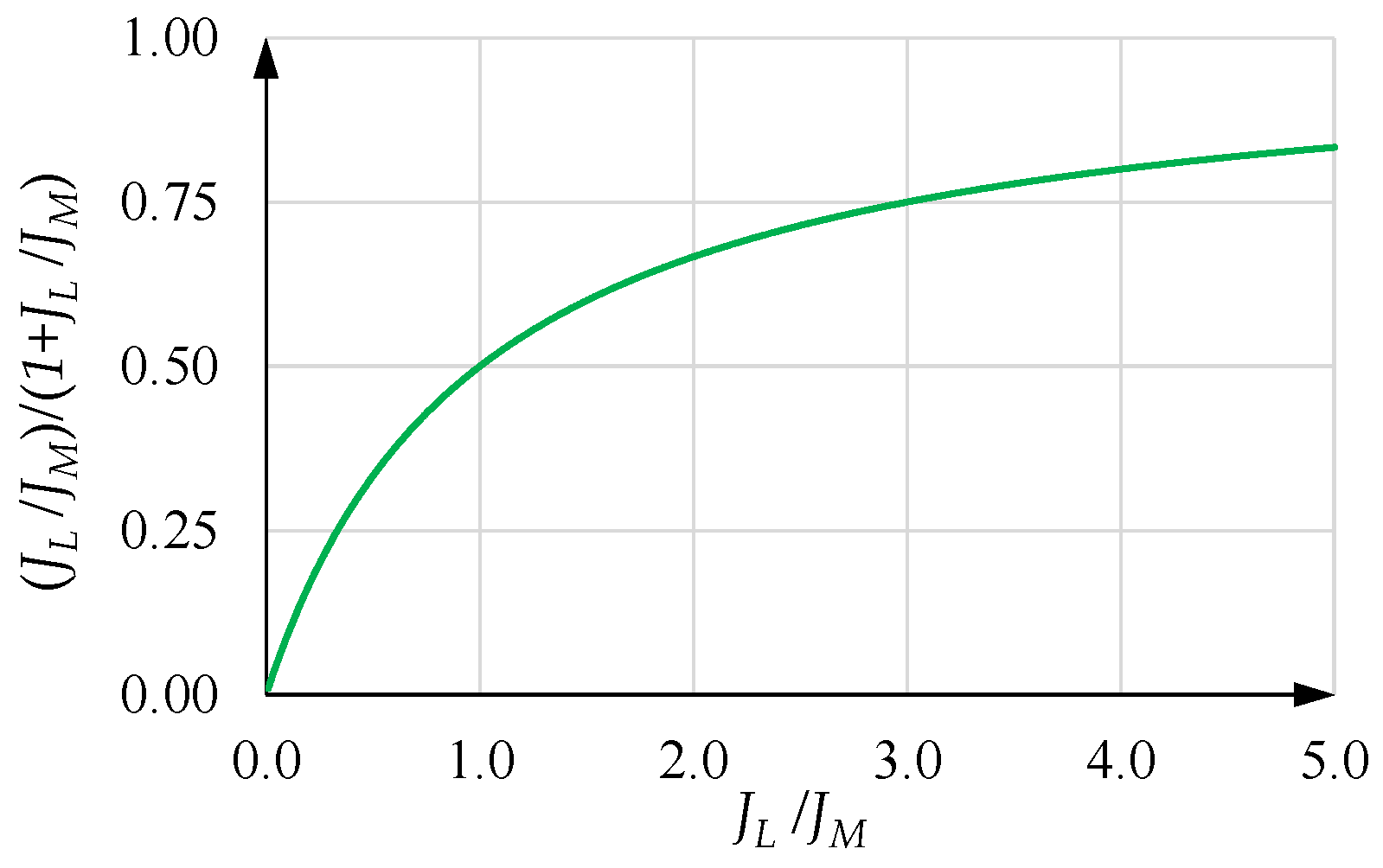
The motor velocity is controlled by a closed chain and its bandwidth and load disturbance attenuation are such that the motor is assumed to perfectly execute the reference velocity profile. In general, the smaller the ratio $J_L/J_M$, the more acceptable these assumptions are. Therefore, the designed acceleration profile $\ddot{\vartheta }\left(t\right)$ becomes a kinematic time-dependent constraint applied to the motor, with respect to which the load oscillates.

The undamped natural frequency is

$${\Omega }_n=\sqrt{\frac{k}{J_L}}$$

(1)

while the corresponding frequency is

$$f_n=\frac{{\Omega }_n}{2\pi }$$

(2)

and the dimensionless structural damping coefficient is

$$\zeta =\frac{c}{2\sqrt{{kJ}_L}}.$$

(3)

The differential equation governing the position ${\vartheta }_l$ of the load with respect to the motor is

$$\frac{{\ddot{\vartheta }}_l}{{\Omega }_n^2}+2\zeta \frac{{\dot{\vartheta }}_l}{{\Omega }_n}+{\vartheta }_l=-\frac{\ddot{\vartheta }}{{\Omega }_n^2}.$$

(4)

The velocity of the load with respect to the motor is governed by the differential equation

$$\frac{{\stackrel{⃛}{\vartheta }}_l}{{\Omega }_n^2}+2\zeta \frac{{\ddot{\vartheta }}_l}{{\Omega }_n}+{\dot{\vartheta }}_l=-\frac{1}{{\Omega }_n^2}\frac{d\ddot{\vartheta }}{dt}.$$

(5)

${\stackrel{⌢}{\dot{\vartheta }}}_l$ is the relative velocity of the load made dimensionless by dividing ${\dot{\vartheta }}_l$ by the maximum velocity ${\dot{\vartheta }}_{max}$ of the motor, which is a specification, i.e.,

$${\stackrel{⌢}{\dot{\vartheta }}}_l=\frac{{\dot{\vartheta }}_l}{{\dot{\vartheta }}_{max}},$$

(6)

and, therefore, Equation (5) becomes

$$\frac{{\ddot{\stackrel{⌢}{\dot{\vartheta }}}}_l}{{\Omega }_n^2}+2\zeta \frac{\dot{\stackrel{⌢}{\dot{\vartheta }}}}{{\Omega }_n}+{\stackrel{⌢}{\dot{\vartheta }}}_l=-\frac{1}{{\dot{\vartheta }}_{max}{\Omega }_n^2}\frac{d\ddot{\vartheta }}{dt}.$$

(7)

The corresponding Laplace transform is

$$\left(\frac{s^2}{{\Omega }_n^2}+2\zeta \frac{s}{{\Omega }_n}+1\right){\stackrel{⌢}{\dot{\Theta }}}_l\left(s\right)=-\frac{s}{{\dot{\vartheta }}_{max}{\Omega }_n^2}\ddot{\Theta }\left(s\right).$$

(8)

2.2. Trapezoidal Acceleration Profile of the Motor for a Rest-to-Velocity Motion

The case of a rest-to-velocity motion with a STAP is now taken into consideration. Apart from its specific importance, as mentioned above, this case is also preparatory to a point-to-point motion.

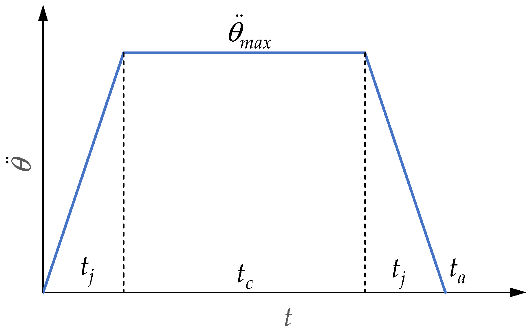
Figure 2 shows a STAP. The acceleration time is equal to $t_a$, while the two jerk times are equal to $t_j$. The two jerk times allow for the reduction of the load oscillations. The acceleration is constant and equal to its maximum value ${\ddot{\vartheta }}_{max}$ during time $t_c$. Because of the symmetry of the acceleration profile, the maximum value $t_{j,max,1}$ that $t_j$ can assume is

$$t_{j,max,1}=\frac{1}{2}{t}_a.$$

(9)

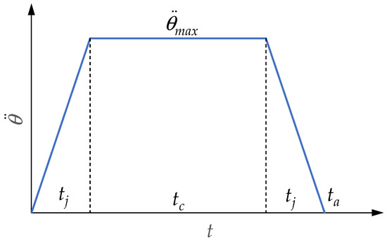
Figure 2. Symmetrical trapezoidal acceleration profile.

The maximum velocity reached by the motor is ${\dot{\vartheta }}_{max}$ and is equal to the area under the acceleration profile. Therefore, its value is

$${\dot{\vartheta }}_{max}={\ddot{\vartheta }}_{max}\left(t_a-t_j\right).$$

(10)

Initially, the specifications are only $t_a$ and ${\dot{\vartheta }}_{max}$. Incidentally, in the end, $t_a$ must be chosen so as to minimize the load settling time. Hence, from Equation (10), the maximum acceleration ${\ddot{\vartheta }}_{max}$ is equal to

$${\ddot{\vartheta }}_{max}=\frac{{\dot{\vartheta }}_{max}}{t_a-t_j}.$$

(11)

The expression of the dimensionless jerk time ${\stackrel{⌢}{t}}_j$ with respect to $t_a$ is

$${\stackrel{⌢}{t}}_j=\frac{t_j}{t_a}.$$

(12)

Therefore, ${\ddot{\vartheta }}_{max}$ assumes the expression

$${\ddot{\vartheta }}_{max}=\frac{{\dot{\vartheta }}_{max}}{t_a}\frac{1}{\left(1-{\stackrel{⌢}{t}}_j\right)},$$

(13)

in which ${\dot{\vartheta }}_{max}/t_a$ is the average acceleration. The dimensionless acceleration coefficient $c_{a,v}$ for velocity is

$$c_{a,v}=\frac{1}{1-{\stackrel{⌢}{t}}_j}.$$

(14)

Therefore, the expression of ${\ddot{\vartheta }}_{max}$ becomes

$${\ddot{\vartheta }}_{max}=c_{a\hspace{0.17em},\hspace{0.33em}v}\frac{{\dot{\vartheta }}_{max}}{t_a}.$$

(15)

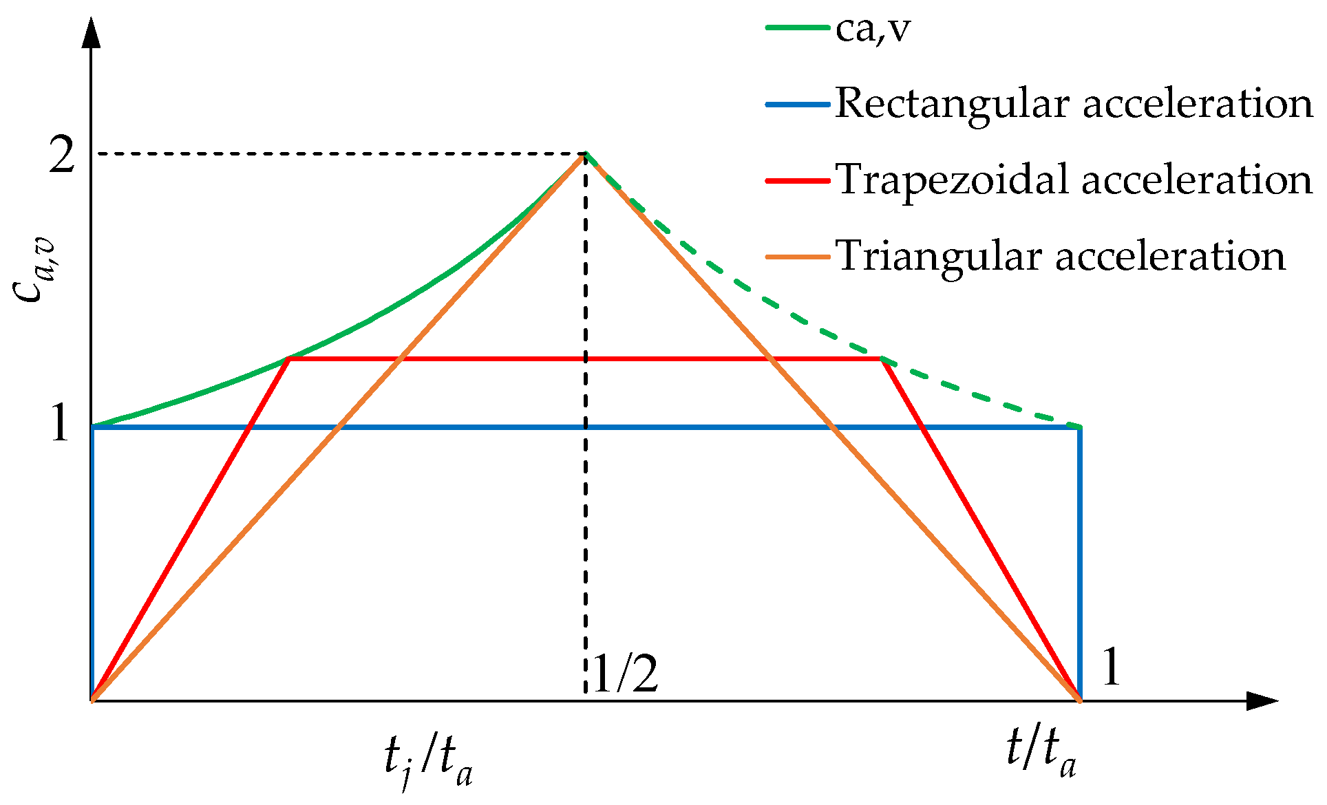
Figure 3 shows the profile of $c_{a,v}$ versus ${\stackrel{⌢}{t}}_j$. In the same figure, a generic STAP is drawn, together with two limit profiles in which, respectively:

1.

${\stackrel{⌢}{t}}_j$ is equal to zero. The acceleration profile is rectangular, i.e., the acceleration is constant throughout the total acceleration time $t_a$ and assumes its minimum value, which is the average value ${\dot{\vartheta }}_{max}/t_a$. The constant acceleration time $t_c$ is equal to $t_a$;

2.

${\stackrel{⌢}{t}}_j$ is equal to one half. The acceleration profile is triangular and the maximum acceleration ${\ddot{\vartheta }}_{max}$ is reached at time $1/2\hspace{0.33em}{t}_a$ and assumes its maximum possible value $2{\dot{\vartheta }}_{max}/t_a$, which is twice the average value ${\dot{\vartheta }}_{max}/t_a$. In this case, the constant acceleration time $t_c$ is equal to zero.

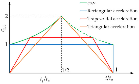
Figure 3. Profile of $c_{a,v}$ versus ${\stackrel{⌢}{t}}_j$ and different dimensionless STAPs.

The jerk is finite unless $t_j$ is equal to zero. From Equations (11) and (12), the maximum value of the jerk is given by

$${\stackrel{⃛}{\vartheta }}_{max}=\frac{{\ddot{\vartheta }}_{max}}{t_j}=\frac{{\dot{\vartheta }}_{max}}{t_j\left(t_a-t_j\right)}=\frac{{\dot{\vartheta }}_{max}}{t_a^2}\frac{1}{{\stackrel{⌢}{t}}_j\left(1-{\stackrel{⌢}{t}}_j\right)}.$$

(16)

Introducing the jerk coefficient $c_{j,v}$ for velocity, its expression is

$$c_{j,v}=\frac{1}{{\stackrel{⌢}{t}}_j\left(1-{\stackrel{⌢}{t}}_j\right)},$$

(17)

and the expression of ${\stackrel{⃛}{\vartheta }}_{max}$ becomes

$${\stackrel{⃛}{\vartheta }}_{max}=c_{j,v}\frac{{\dot{\vartheta }}_{max}}{t_a^2}.$$

(18)

Figure 4 shows $c_{j,v}$ versus ${\stackrel{⌢}{t}}_j$ and the corresponding jerk profiles for a generic STAP, for a rectangular one, and for a triangular one.

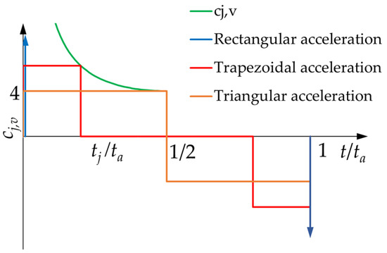
Figure 4. Profile of $c_{j,v}$ versus ${\stackrel{⌢}{t}}_j$ and different dimensionless jerk profiles.

Now, in addition to $t_a$ and ${\dot{\vartheta }}_{max}$, there is another specification: the maximum value ${\ddot{\vartheta }}_{Max}$ that the maximum acceleration ${\ddot{\vartheta }}_{max}$ can take. The value of ${\ddot{\vartheta }}_{Max}$ is specified with a margin of uncertainty. In fact, it can depend on the following:

-

The maximum motor torque $M_{m,Max}$ caused by the electronic driver feeding the motor. Nevertheless, with respect to the value

$${\ddot{\vartheta }}_{Max}=\frac{M_{m,Max}}{J_M+J_L},$$

(19)

which is the corresponding acceleration of the nodal section, it is necessary to take into account both the oscillations of the motor torque caused by load vibrations, resulting from an incorrect estimate of the natural frequency, and those caused by the fact that the motor cannot perfectly perform the reference velocity, even at no load;

-

The transmission and load limits (the transmission is not represented in the model in Figure 1); however, in this case once again, the load vibrations must be taken into account.

In any case, ${\ddot{\vartheta }}_{Max}$ is generalized to the motor. It is obvious that

$${\ddot{\vartheta }}_{max}\le {\ddot{\vartheta }}_{Max}.$$

(20)

From ${\ddot{\vartheta }}_{Max}$ it is possible to find the minimum value $t_{a,min}$ [20] that the specified acceleration time $t_a$ can take, when the maximum velocity ${\dot{\vartheta }}_{max}$ is reached with constant acceleration ${\ddot{\vartheta }}_{Max}$:

$$t_{a,min}=\frac{{\dot{\vartheta }}_{max}}{{\ddot{\vartheta }}_{Max}}.$$

(21)

Thus, $t_a$ satisfies the inequality

$$t_a\ge t_{a,min}.$$

(22)

Achieving the acceleration limit acts to minimize the acceleration time $t_a$, but it restricts the family of STAPs capable of doing so. In fact, if ${\ddot{\vartheta }}_{Max}$ is such that

$${\dot{\vartheta }}_{max}/t_a\le {\ddot{\vartheta }}_{Max}\le 2{\dot{\vartheta }}_{max}/t_a,$$

(23)

then

$${\dot{\vartheta }}_{max}/{\ddot{\vartheta }}_{Max}\le t_a\le 2{\dot{\vartheta }}_{max}/{\ddot{\vartheta }}_{Max},$$

(24)

i.e., keeping in mind Equation (21),

$$t_{a,min}\le t_a\le 2t_{a,min}.$$

(25)

Therefore, to achieve the velocity ${\dot{\vartheta }}_{max}$, the possibility of reaching the acceleration limit ${\ddot{\vartheta }}_{Max}$ is limited to STAPs whose acceleration time $t_a$ satisfies the inequalities in Equation (25).

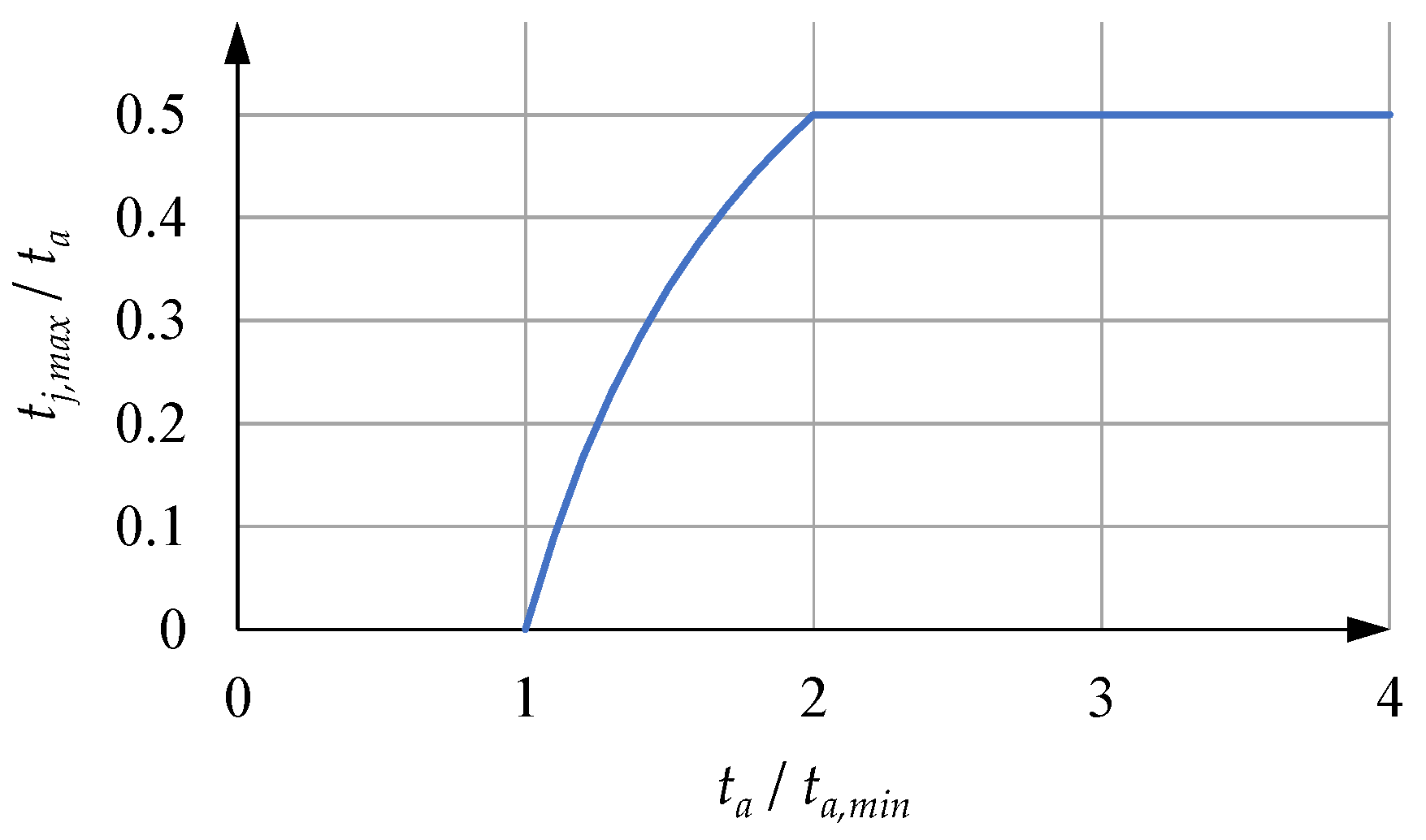
For a given $t_a$, a maximum value ${\stackrel{⌢}{t}}_{j,max,2}$ of ${\stackrel{⌢}{t}}_j$ derives from this new constraint. It can be obtained from Equation (13), by isolating ${\stackrel{⌢}{t}}_j$ and assuming that ${\ddot{\vartheta }}_{max}$ is equal to ${\ddot{\vartheta }}_{Max}$:

$${\stackrel{⌢}{t}}_{j,max,2}=1-\frac{{\dot{\vartheta }}_{max}}{{\ddot{\vartheta }}_{Max}{t}_a}=1-\frac{t_{a,min}}{t_a}\le \frac{1}{2},$$

(26)

or, in dimensional terms,

$$t_{j,max,2}=t_a-t_{a,min}\le t_{a,min}.$$

(27)

If the inequalities in Equation (25) are met, both the inequalities in Equations (9) and (27) must be satisfied and the global maximum value $t_{j,max}$ of $t_j$ is

$$t_{j,max}=min\left(t_{j,max,1},t_{j,max,2}\right)=t_{j,max,2}.$$

(28)

Its value reaches one half of $t_a$ in the limit condition

$$t_a=2t_{a,min}.$$

(29)

If the inequalities in Equation (25) are satisfied and the acceleration limit ${\ddot{\vartheta }}_{Max}$ is reached, the acceleration profile always shows its second vertex V at time $t_{a,min}$, as is shown in Figure 5 for a generic value of $t_a$ and for two limit cases, when $t_a$ is equal to $t_{a,min}$ and 2$t_{a,min}$, respectively. It is then evident that, in general, the constant acceleration time $t_c$ is less than $t_{a,min}$, unless $t_a$ is equal to $t_{a,min}$ and thus $t_j$ is equal to zero. Furthermore, if Equation (29) is met, the acceleration profile is triangular and $t_c$ is equal to zero.

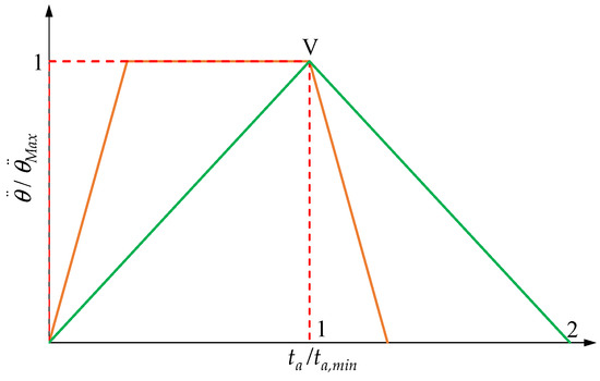
Figure 5. Dimensionless trapezoidal acceleration profiles when the inequalities in Equation (25) are met.

On the contrary, if

$$t_a>2t_{a,min},$$

(30)

to achieve the maximum velocity ${\dot{\vartheta }}_{max}$, the acceleration limit ${\ddot{\vartheta }}_{Max}$ cannot be reached by a STAP. The STAP that reaches ${\ddot{\vartheta }}_{Max}$ with the maximum value of $t_a$ is the triangular example in Figure 5, when $t_a$ is equal to $2t_{a,min}$. When $t_a$ satisfies the inequality in Equation (30), among all STAPs that allow for the same maximum velocity ${\dot{\vartheta }}_{max}$, the triangular acceleration profile reaches the maximum possible acceleration ${\ddot{\vartheta }}_{max,M}$ given by

$${\ddot{\vartheta }}_{max,M}=\frac{2{\ddot{\vartheta }}_{Max}}{\frac{t_a}{t_{a,min}}},$$

(31)

which is less than ${\ddot{\vartheta }}_{Max}$.

In this case, the maximum value of $t_j$ is

$${\stackrel{⌢}{t}}_{j,max}=\frac{1}{2}.$$

(32)

Figure 6 shows the profile of ${\stackrel{⌢}{t}}_{j,max}$ versus $t_a/t_{a,min}$.

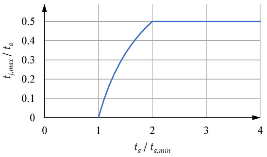
Figure 6. Profile of ${\stackrel{⌢}{t}}_{j,max}$ versus $t_a/t_{a,min}$.

It is evident that, within the range defined by the inequalities in Equation (25), there are also other STAPs whose area is equal to ${\dot{\vartheta }}_{max}$, but whose maximum acceleration is less than ${\ddot{\vartheta }}_{Max}$. Nevertheless, with the same value of $t_j$, these profiles require a greater value of $t_a$ than profiles that reach ${\ddot{\vartheta }}_{Max}$. An example is given by the rectangular acceleration profiles ($t_j$ is equal to zero), whose maximum acceleration ${\ddot{\vartheta }}_{max,m}$ is

$${\ddot{\vartheta }}_{max,m}=\frac{{\ddot{\vartheta }}_{Max}}{\frac{t_a}{t_{a,min}}}.$$

(33)

With a given $t_a$, this is the minimum possible maximum acceleration that satisfies the inequalities in Equation (25) (the violet curve in Figure 7). A rectangular acceleration profile with a given value of $t_a$ that satisfies the inequality in Equation (30) is still characterized by the minimum possible maximum acceleration ${\ddot{\vartheta }}_{max,m}$, given by Equation (33).

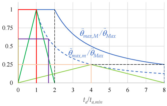
Figure 7. Profiles of ${\ddot{\vartheta }}_{max,M}/{\ddot{\vartheta }}_{Max}$ (continuous blue curve) and ${\ddot{\vartheta }}_{max,m}/{\ddot{\vartheta }}_{Max}$ (dashed blue curve) versus $t_a/t_{a,min}$; dimensionless triangular and rectangular acceleration profiles.

Figure 7 shows the aforementioned profiles using dimensionless quantities. It can be noted that the right vertex of a rectangular acceleration profile is also the vertex of the triangular profile with a double value of $t_a$.

The dark green triangle is the acceleration limit profile with $t_a$ equal to $2t_{a,min}$, the light green curve is a triangular acceleration profile with $t_a$ greater than $2t_{a,min}$, the red rectangle is the acceleration profile with $t_a$ equal to $t_{a,min}$, and the pink rectangle has an acceleration time that is half that of the light green one. The violet rectangle is characterized by a value of $t_a$ less than $2t_{a,min}$ and therefore does not reach ${\ddot{\vartheta }}_{Max}$.

2.3. Suppression of the Residual Oscillations of the Load

The natural frequency $f_n$ and the dimensionless damping coefficient $\zeta$ are assumed not to be known with any accuracy, even though $\zeta$ is much smaller than one. In the design of the STAP, $\zeta$ is assumed to be equal to zero, while $f_{n,e}$ is an estimated value of $f_n$.

With the STAP, the Laplace transform of the differential Equation (7) becomes

$$\left(\frac{s^2}{{\Omega }_n^2}+2\zeta \frac{s}{{\Omega }_n}+1\right){\stackrel{⌢}{\dot{\Theta }}}_l\left(s\right)=-\frac{s{\ddot{\vartheta }}_{max}}{{\dot{\vartheta }}_{max}{t}_a{\stackrel{⌢}{t}}_j{s}^2{\Omega }_n^2}\left[1-e^{-s{t}_a{\stackrel{⌢}{t}}_j}-e^{-s{t}_a\left(1-{\stackrel{⌢}{t}}_j\right)}+e^{-s{t}_a}\right],$$

(34)

and, keeping in mind Equations (13) and (17), the result is

$$\left(\frac{s^2}{{\Omega }_n^2}+2\zeta \frac{s}{{\Omega }_n}+1\right){\stackrel{⌢}{\dot{\Theta }}}_l\left(s\right)=-\frac{t_a{c}_{j,v}}{s{t}_a{\Omega }_n^2{t}_a^2}\left[1-e^{-s{t}_a{\stackrel{⌢}{t}}_j}-e^{-s{t}_a\left(1-{\stackrel{⌢}{t}}_j\right)}+e^{-s{t}_a}\right].$$

(35)

If a harmonic analysis is carried out, substituting s for its imaginary part $i\Omega$, the result is

$$\left(1-\frac{{\Omega }^2}{{\Omega }_n^2}+i2\zeta \frac{\Omega }{{\Omega }_n}\right){\stackrel{⌢}{\dot{\Theta }}}_l\left(i\Omega \right)=i\frac{t_a{c}_{j,v}}{\Omega t_a{\Omega }_n^2{t}_a^2}\left[1-e^{-i\Omega t_a{\stackrel{⌢}{t}}_j}-e^{-i\Omega t_a\left(1-{\stackrel{⌢}{t}}_j\right)}+e^{-i\Omega t_a}\right].$$

(36)

The exciting term E, on the right-hand side, is equal to

$$E=i\frac{t_a{c}_{j,v}}{\Omega t_a{\Omega }_n^2{t}_a^2}\left[1-e^{-i\Omega t_a{\stackrel{⌢}{t}}_j}-e^{-i\Omega t_a\left(1-{\stackrel{⌢}{t}}_j\right)}+e^{-i\Omega t_a}\right].$$

(37)

If the system has no damping, $\zeta$ is equal to zero and Equation (36) becomes

$$\left(1-\frac{{\Omega }^2}{{\Omega }_n^2}\right){\stackrel{⌢}{\dot{\Theta }}}_l\left(i\Omega \right)=i\frac{t_a{c}_{j,v}}{\Omega t_a{\Omega }_n^2{t}_a^2}\left[1-e^{-i\Omega t_a{\stackrel{⌢}{t}}_j}-e^{-i\Omega t_a\left(1-{\stackrel{⌢}{t}}_j\right)}+e^{-i\Omega t_a}\right].$$

(38)

Under these conditions ($\zeta$ is equal to zero), in order to make the residual vibrations zero, the system is considered in resonance conditions, i.e., $\Omega$ is equal to ${\Omega }_n$. The necessary consequences are drawn for the exciting term E, whose absolute value must be zero in order to avoid the introduction of excitation energy into the system at the undamped natural frequency ${\Omega }_n$ [20].

Keeping in mind Equation (2), the exciting term E becomes

$$E=i\frac{t_a{c}_{j,v}}{{\left(2\pi \right)}^3{f}_n^3{t}_a^3}\left[1-e^{-i2\pi \left(f_n{t}_a\right){\stackrel{⌢}{t}}_j}-e^{-i2\pi \left(f_n{t}_a\right)\left(1-{\stackrel{⌢}{t}}_j\right)}+e^{-i2\pi \left(f_n{t}_a\right)}\right].$$

(39)

The dimensionless term

$$r_{n,a}=f_n{t}_a$$

(40)

is the number of undamped free oscillations of the system during time $t_a$. It is not necessarily an integer number and increases with $f_n$ and $t_a$.

In Equation (39), E is proportional to $t_a$ and depends on $f_n{t}_a$ and ${\stackrel{⌢}{t}}_j$ in a complex way. It also depends on ${\stackrel{⌢}{t}}_j$ through $c_{j,v}$ (Equation (17)). If u denotes the term in brackets in Equation (39), i.e.,

$$u=1-e^{-i2\pi \left(f_n{t}_a\right){\stackrel{⌢}{t}}_j}-e^{-i2\pi \left(f_n{t}_a\right)\left(1-{\stackrel{⌢}{t}}_j\right)}+e^{-i2\pi \left(f_n{t}_a\right)},$$

(41)

the exciting term E can also be written as

$$E=i\frac{t_a{c}_{j,v}}{{\left(2\pi \right)}^3{\left(f_n{t}_a\right)}^3}u.$$

(42)

As said above, in order to avoid residual vibrations the absolute value of the exciting term E must be equal to zero at the undamped natural frequency ${\Omega }_n$. The analysis of Equation (42) shows that what must be equal to zero is just u, which depends on $r_{n,a}$ and ${\stackrel{⌢}{t}}_j$, except for the particular case in which ${\stackrel{⌢}{t}}_j$ is equal to zero and $c_{j,v}$ tends to infinity.

For a given value of $r_{n,a}$, the absolute value of u can be represented as a function of ${\stackrel{⌢}{t}}_j$, while for given values of $r_{n,a}$ and $t_a$, the absolute value of E can be represented as a function of ${\stackrel{⌢}{t}}_j$.

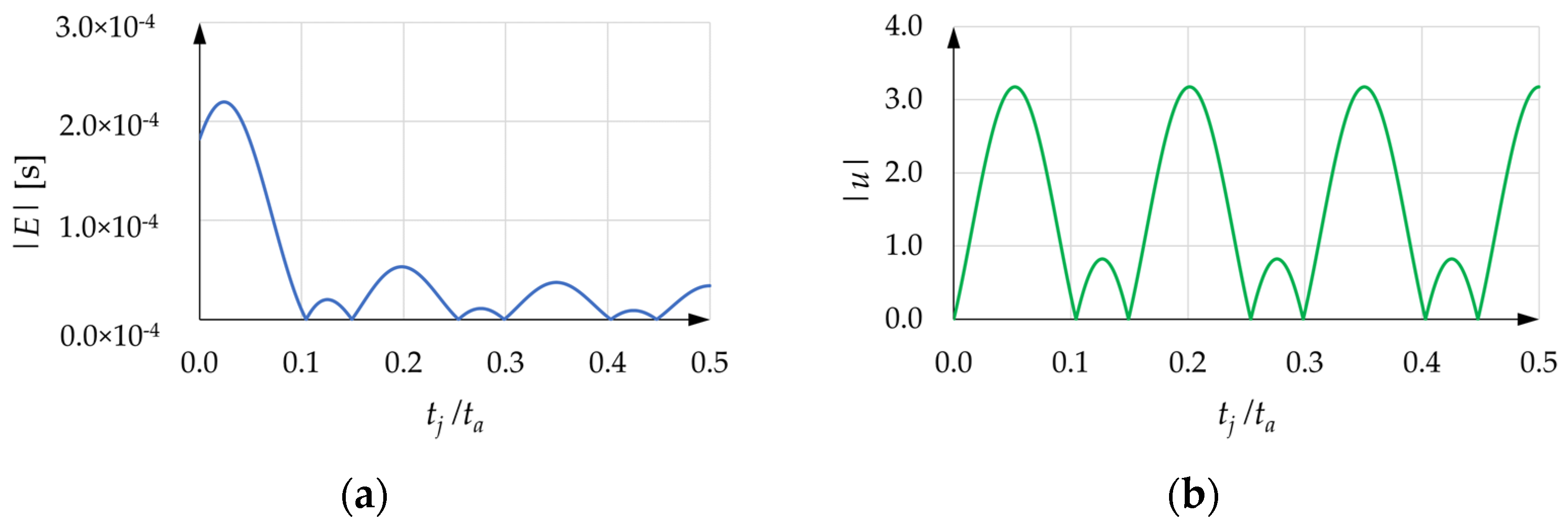
Figure 8a,b show an example of the absolute values of E and u versus ${\stackrel{⌢}{t}}_j$ with $r_{n,a}$ equal to 6.7 and $t_a$ equal to 0.2 s. The maximum abscissa is obviously equal to 0.5. If $t_a$ is less than $2t_{a,min}$, only the part of the curves whose abscissa is not greater than ${\stackrel{⌢}{t}}_{j,max}$ must be considered. This means that, in this case, for a given $t_a$, it is advisable to draw a vertical line whose abscissa ${\stackrel{⌢}{t}}_{j,max}$ is smaller than one half, and to only consider the part of the curves that is not to the right of this line.

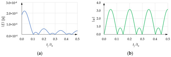
Figure 8. (a) Absolute value of E versus ${\stackrel{⌢}{t}}_j$ ($r_{n,a}$ equal to 6.7, $t_a$ equal to 0.2 s); (b) corresponding absolute value of u versus ${\stackrel{⌢}{t}}_j$.

The diagrams of |E| and |u| show the same zeros, regularly spaced, apart from the abscissa ${\stackrel{⌢}{t}}_j$ equal to zero, where |u| is always equal to zero, whereas |E| can assume a positive value. To avoid residual vibrations of the load, ${\stackrel{⌢}{t}}_j$ should assume the values ${\stackrel{⌢}{t}}_{j,0}$ corresponding to the zeros of |E|.

The abscissas ${\stackrel{⌢}{t}}_{j,0}$ of these zeros respect the following rules: The positive real number $r_{n,a}$ can be represented as the sum of its integer part $int\left(r_{n,a}\right)$ and its decimal part $dec\left(r_{n,a}\right)$:

$$r_{n,a}=int\left(r_{n,a}\right)+dec\left(r_{n,a}\right)$$

(43)

For example, for $r_{n,a}$ equal to 6.7, $int\left(r_{n,a}\right)$ is equal to 6.0 and $dec\left(r_{n,a}\right)$ is equal to 0.7. The abscissas ${\stackrel{⌢}{t}}_{j,0}$ of the zeros correspond to the expression

$${\stackrel{⌢}{t}}_{j,0}=\left[k_j+\delta \cdot dec\left(r_{n,a}\right)\right]\frac{1}{r_{n,a}},$$

(44)

where k_j is a progressive integer number and $\delta$ alternately takes the values one and zero (see Appendix A). Table 1 shows the progressive values of the couples $\left(k_j,\delta \right)$.

Table 1. Progressive values of the couples $\left(k_j,\delta \right)$.

n	kj	$\mathit{\delta }$
1	0	1
2	1	0
3	1	1
4	2	0
5	2	1
6	3	0
7	3	1
8	…	…

The couple $\left(k_j,\delta \right)$ cannot assume the value $\left(0, 0\right)$, i.e., k_j and $\delta$ cannot be simultaneously null. Nevertheless, ${\stackrel{⌢}{t}}_{j,0}$ can assume the value zero, and this happens when k_j is equal to zero, but $\delta$ is equal to one and $dec\left(r_{n,a}\right)$ is equal to zero. In this case, $r_{n,a}$ is an integer number, and the couple $\left(k_j,\delta \right)$ equal to $\left(0, 1\right)$ gives ${\stackrel{⌢}{t}}_{j,0}$ equal to zero, which means that the acceleration profile is rectangular.

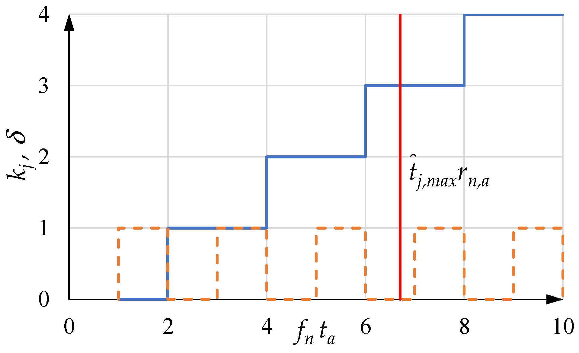
Figure 9 shows the values of k_j and $\delta$ versus the abscissa $r_{n,a}$. The diagrams in Figure 9 must be read according to the following rule: once the vertical line corresponding to the actual value of ${\stackrel{⌢}{t}}_{j,max}{r}_{n,a}$ is drawn, all the couples of k_j and $\delta$ that are not to the right of this vertical must be taken into consideration.

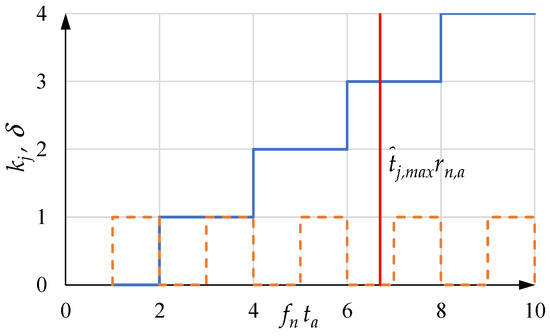
Figure 9. Values of k_j and δ versus the abscissa $r_{n,a}$.

To prevent ${\stackrel{⌢}{t}}_{j,0}$ from taking a value greater than ${\stackrel{⌢}{t}}_{j,max}$:

1.

The integer k_j assumes a maximum value $k_{j,max}$ given by

$$k_{j,max}=int\left[{\stackrel{⌢}{t}}_{j,max}\cdot int\left(r_{n,a}\right)\right];$$

(45)

2.

$\delta$ assumes a final value ${\delta }_f$ given by the integer (zero or one) closest to ${\stackrel{⌢}{t}}_{j,max}{r}_{n,a}-k_{j,max}$, a function that is expressed by round:

$${\delta }_f=round\left({\stackrel{⌢}{t}}_{j,max}{r}_{n,a}-k_{j,max}\right).$$

(46)

For example, with $r_{n,a}$ equal to 6.7 and ${\stackrel{⌢}{t}}_{j,max}$ equal to 0.5, $k_{j,max}$ is equal to 3 and ${\delta }_f$ is equal to 0. These results can be compared with the zeros in Figure 8.

The value

$${\stackrel{⌢}{t}}_{j,0,1}=\frac{1}{r_{n,a}}$$

(47)

is here called the fundamental value.

The values

$${\stackrel{⌢}{t}}_{j,0,k}=\frac{k_j}{r_{n,a}} \mathrm{with} k_j=1, 2, \dots , k_{j,max},$$

(48)

are multiples of the fundamental value and they correspond to progressively increasing values of ${\stackrel{⌢}{t}}_j$. The remaining values $\frac{k+dec\left(r_{n,a}\right)}{r_{n,a}}$ with $k_j$ equal to 0, 1, …, $k_{j,max}$, are left side-band values of ${\stackrel{⌢}{t}}_{j,0,k}$. Only the value $\frac{dec\left(r_{n,a}\right)}{r_{n,a}}$ corresponds to a value of ${\stackrel{⌢}{t}}_j$ that is less than the fundamental value.

The important thing is that, from Equation (44), the dimensional values of $t_j$ corresponding to the zeros of the exciting term only depend on the natural frequency $f_n$, and not on the acceleration time $t_a$ (apart from the values of $k_{j,max}$ and ${\delta }_f$ if $t_a$ is less than 2$t_{a,min}$):

$$t_{j,0}=\left[k_j+\delta \cdot dec\left(r_{n,a}\right)\right]\frac{1}{f_n}.$$

(49)

The fundamental value of $t_{j,0}$ is

$$t_{j,0,1}=\frac{1}{f_n}.$$

(50)

In general, the number $r_{n,j}$ of undamped free oscillations during time $t_j$ is

$$r_{n,j}=f_n{t}_j.$$

(51)

Hence, the number $r_{n,j,0}$ of undamped free oscillations during time $t_{j,0}$ is

$$r_{n,j,0}=f_n{t}_{j,0}=k_j+\delta \cdot dec\left(r_{n,a}\right).$$

(52)

When $\delta$ is equal to zero, the result is

$$r_{n,j,0}=1, 2, \dots , k_{j,max}.$$

(53)

This is an important result because it means that there is an integer number of undamped free oscillations within the jerk times $t_{j,0,k}$ that corresponds to those zeros of the exciting term, whose abscissa is a multiple of the fundamental value.

2.4. Sensitive Curves

To design the acceleration profile, a value $f_{n,e}$ of the natural frequency $f_n$ must be estimated. Even though at frequency $f_{n,e}$ the amplitude of the residual oscillations is null, when $f_n$ is different from $f_{n,e}$, i.e., $f_n/f_{n,e}$ is different from one, load acceleration oscillations generally occur during time $t_c$ and the amplitude of the residual oscillations is different from zero and can be too large. It is therefore necessary that there is a sufficiently large range of frequencies around $f_{n,e}$, both for values greater and less than $f_{n,e}$, in which the amplitude of the residual oscillations is sufficiently small. The SC shows the maximum absolute value $\left|{\dot{\vartheta }}_{l,r}\right|$ of the residual oscillations of the load velocity, made dimensionless with respect to the maximum value ${\dot{\vartheta }}_{max}$ of the motor velocity (which is also the steady-state velocity of the load), versus $f_n/f_{ne}$.

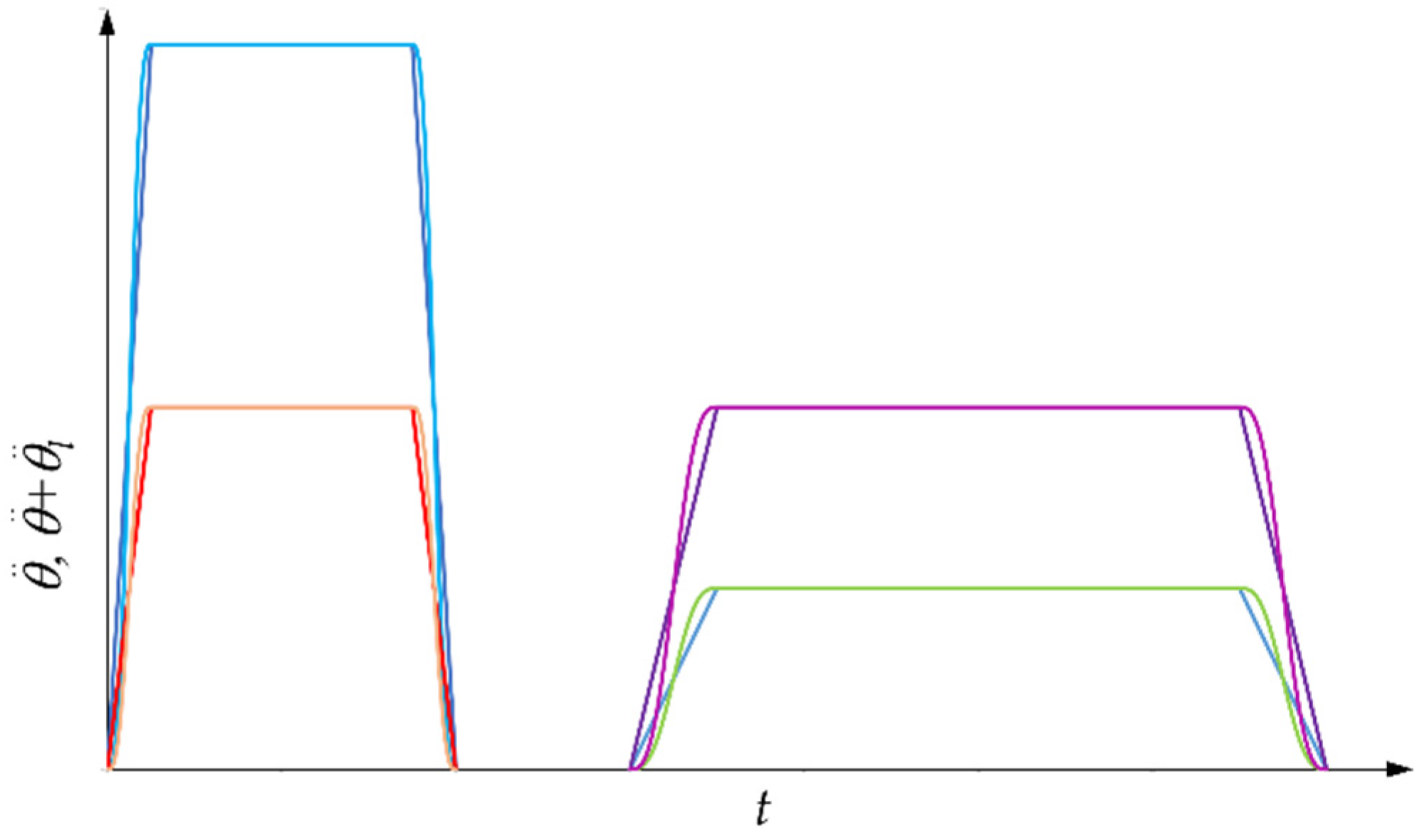
It is interesting to note that with a given value of $k_j$ and $\delta$ equal to zero, the SCs do not change if $f_n$ and $t_a$ change, while maintaining their product $f_n{t}_a$ constant. In this case,

$$f_n{t}_a=f_n\left(t_c+2t_j\right)=f_n\left(t_c+2\frac{k_j}{f_n}\right)=f_n{t}_c+2k_j.$$

(54)

Hence, $f_n{t}_c$ is also constant, i.e., $t_a$, $t_c$, and $t_j$ are inversely proportional to $f_n$. In general, for a given value of $f_n{t}_a$, equal to $r_{n,a}$, and of $k_j$, $t_a$ is equal to $r_{n,a}/f_n$, $t_j$ is equal to $k_j/f_n$ and $t_c$ is equal to $\left(r_{n,a}-2k_j\right)/f_n$. The latter value implies that

$$r_{n,a}\ge 2k_j.$$

(55)

Furthermore, this result is independent of ${\dot{\vartheta }}_{max}$ and ${\ddot{\vartheta }}_{max}$, whose ratio is inversely proportional to $f_n$ (Equation (11)). Figure 10 shows the above. With $k_j$ equal to one, the red and blue acceleration profiles refer to a given value of $f_n$ and $t_a$, but with values of ${\dot{\vartheta }}_{max}$ and ${\ddot{\vartheta }}_{max}$ being twice as large for the blue profile as for the red profile. The green and the violet acceleration profiles refer to the frequency $f_n/2$ and the acceleration time $2t_a$, with the same values of ${\dot{\vartheta }}_{max}$ as the red and blue profile, respectively. The green and the violet profiles have a value of ${\ddot{\vartheta }}_{max}$ that is half that of the red and blue profiles, respectively. All these profiles have the same $f_n{t}_a$ and $k_j$, and generate the same SC.

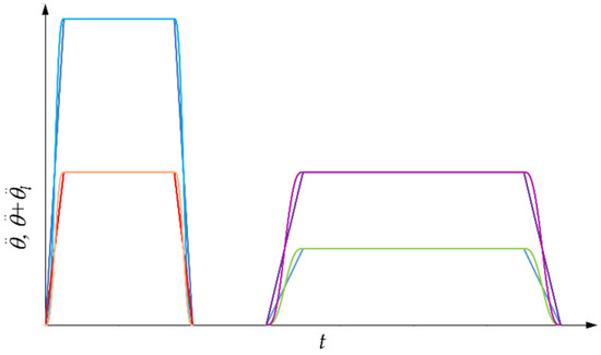
Figure 10. Different motor and load acceleration profiles with the same SC.

This means that the SCs depend only on the product $f_n{t}_a$ (and $k_j$). This property reduces the number of possible SCs to be studied. If the system is damped, the SCs also depend on $\zeta$.

In this regard, it should be remembered that the load is elastically connected to the motor, which has a complex closed velocity chain, and therefore has some damping. Consequently, even if the structural damping coefficient c is zero, the load oscillations are damped, with a damping that depends on the ratio $J_L/J_M$, $k$, the architecture of the control chain, and the tuning of its parameters. In any case, this dimensionless damping is almost negligible, but it makes the SCs smoother and, except around the zeros of the theoretical curves, lower than these.

In the particular case in which $t_a$ is less than or equal to $2t_{a,min}$ and the acceleration limit ${\ddot{\vartheta }}_{Max}$ is reached,

$$f_n{t}_a=f_n\left(t_{a,min}+t_j\right)=f_n\left(t_{a,min}+\frac{k_j}{f_n}\right)=f_n{t}_{a,min}+k_j,$$

(56)

and there is a single frequency $f_n$ corresponding to the given $f_n{t}_a$.

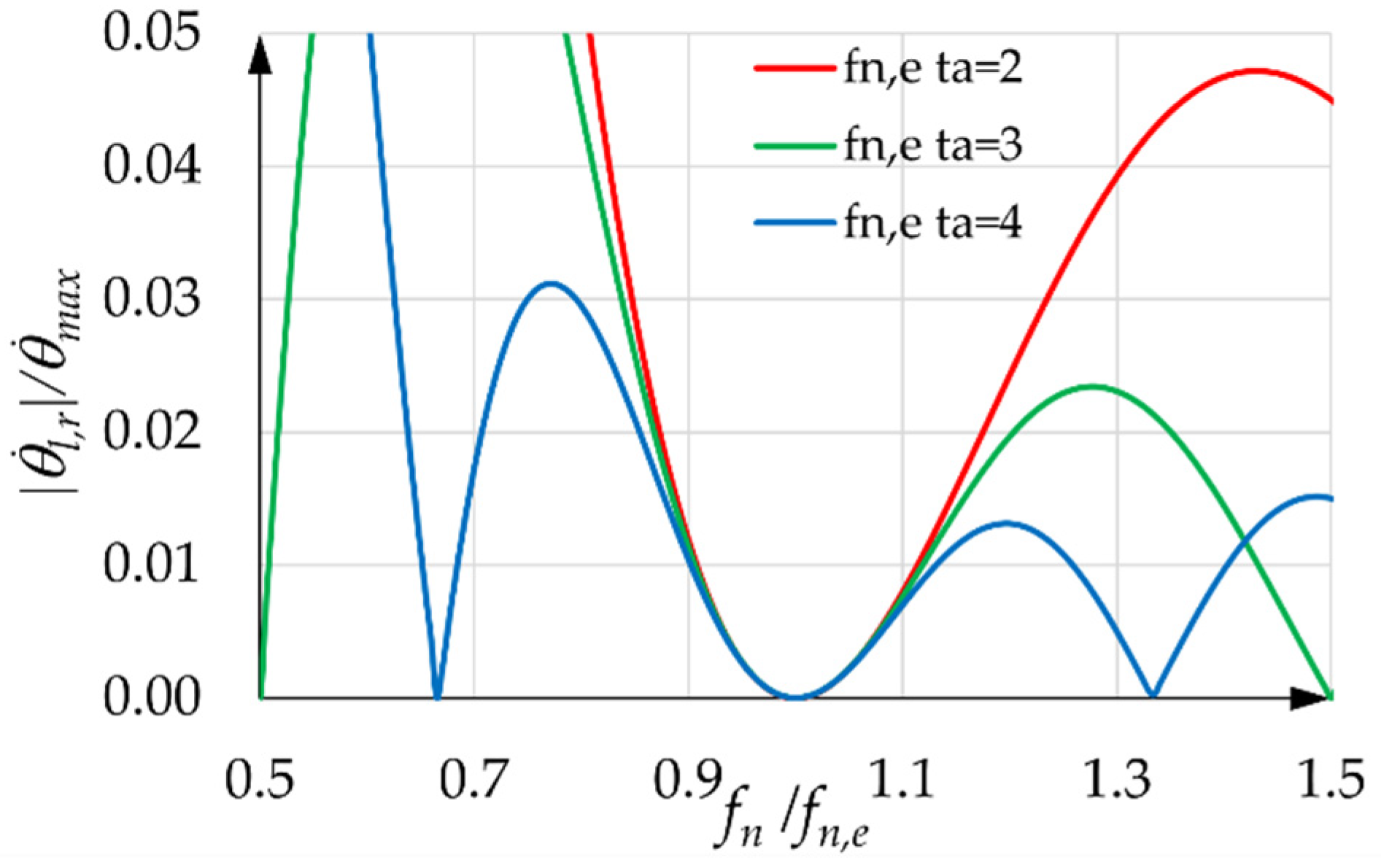
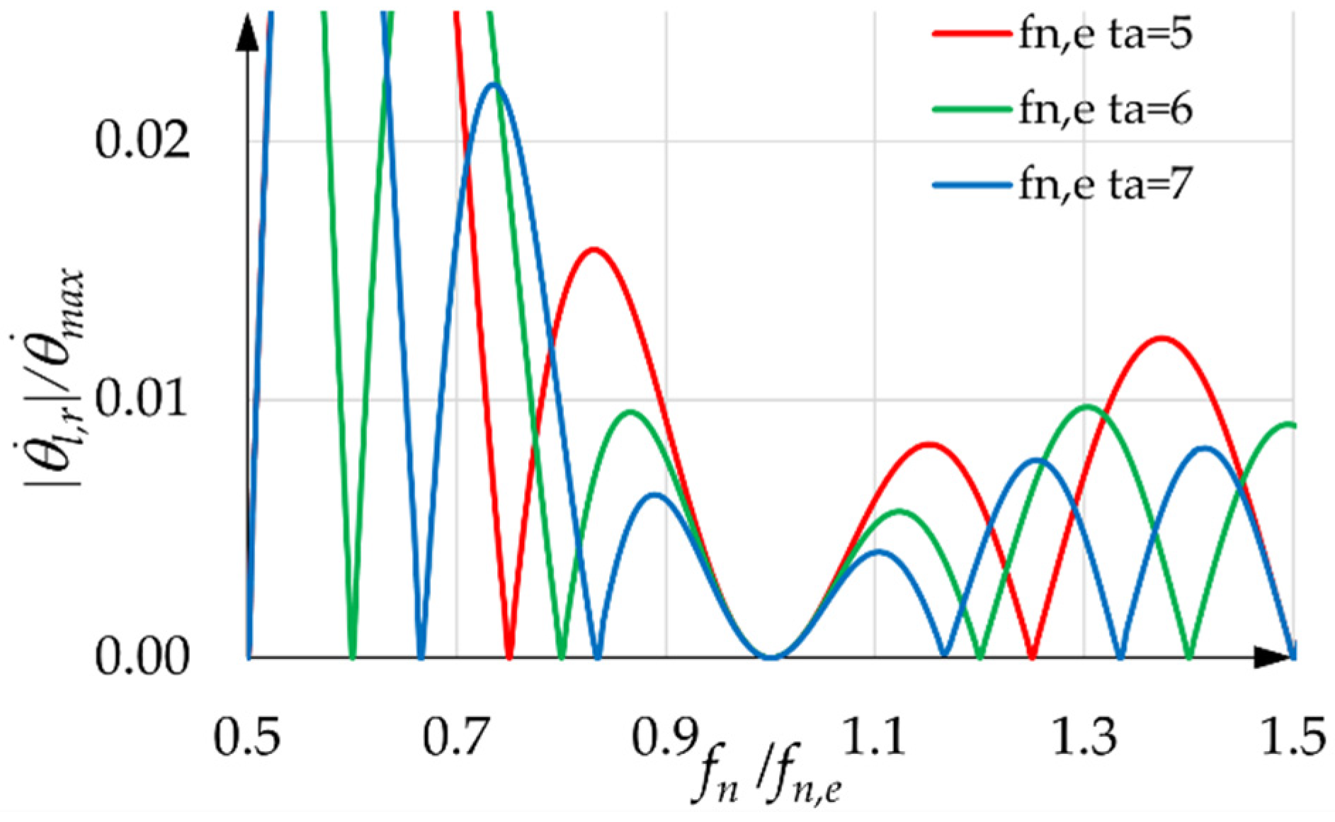
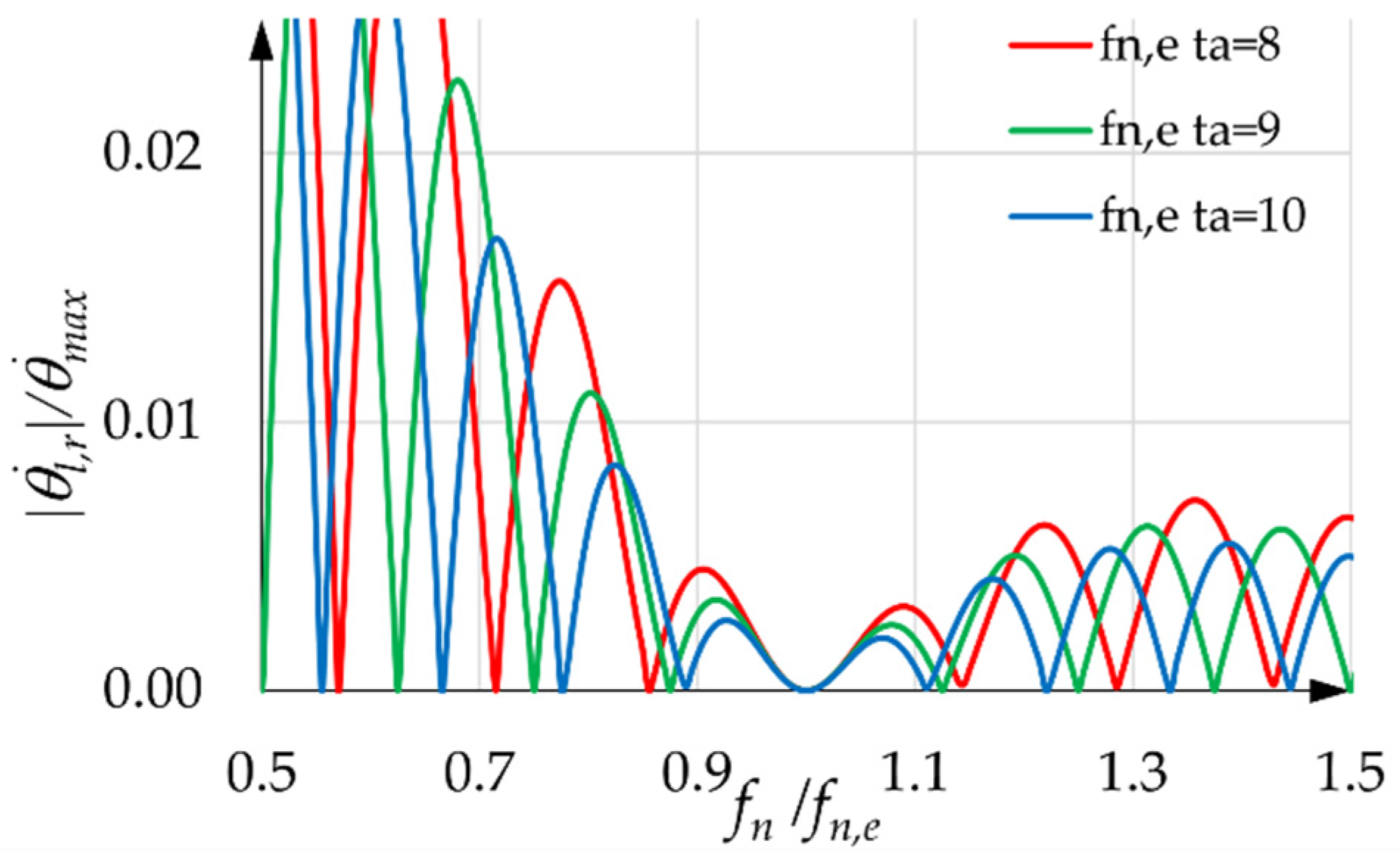
Figure 11, Figure 12 and Figure 13 show the SCs for $k_j$ equal to one and for different values of $f_n{t}_a$. These values are integers only for the sake of simplicity. It is evident that, for a given $f_n$, the SCs improve, from all points of view, as $t_a$ increases. With a given value of $k_j$ and with $\delta$ equal to zero, the SCs show a horizontal tangent at the abscissa one, implying that there is a non-small range around one where the residual velocity oscillation is very small. These SCs were found by assuming that the motor performs the STAP perfectly and neglecting the damping of the motor’s closed velocity chain. Therefore, these curves are a bit higher than the real ones. The theoretical expressions of the SCs, when $\zeta$ is equal to zero and $f_{n,e}{t}_a$ and $k_j$ are assigned, can be found in Appendix B.

Figure 11. SCs with $k_j$ equal to one and $f_{n,e}{t}_a$ equal to two, three, and four.

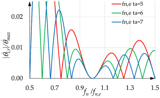
Figure 12. SCs with $k_j$ equal to one and $f_{n,e}{t}_a$ equal to five, six, and seven.

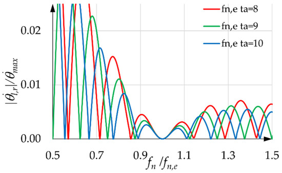
Figure 13. SCs with $k_j$ equal to one and $f_{n,e}{t}_a$ equal to eight, nine, and ten.

3. Results

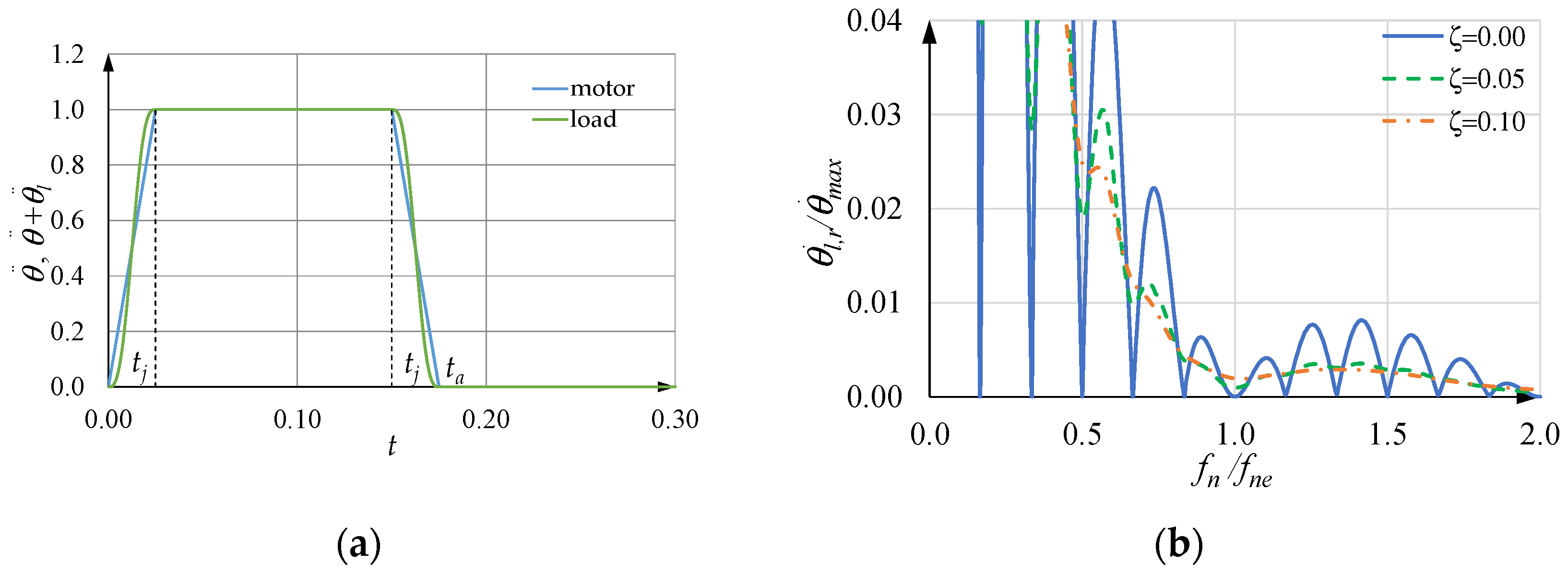
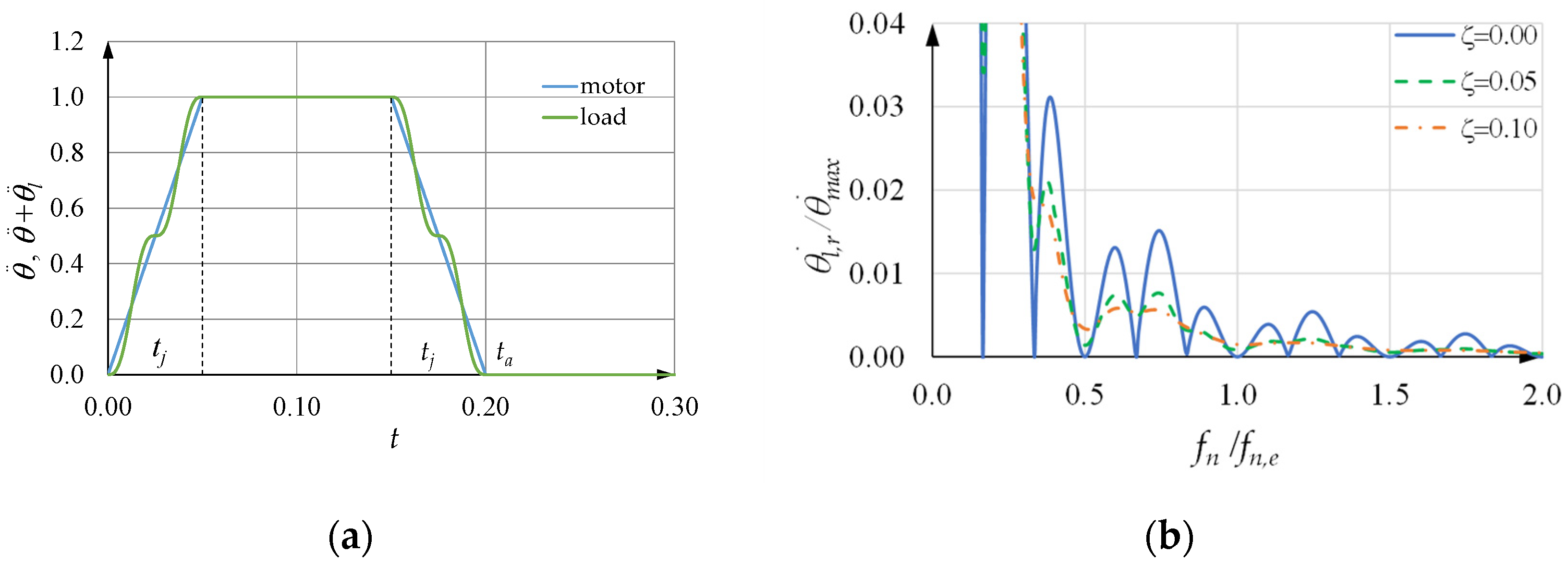
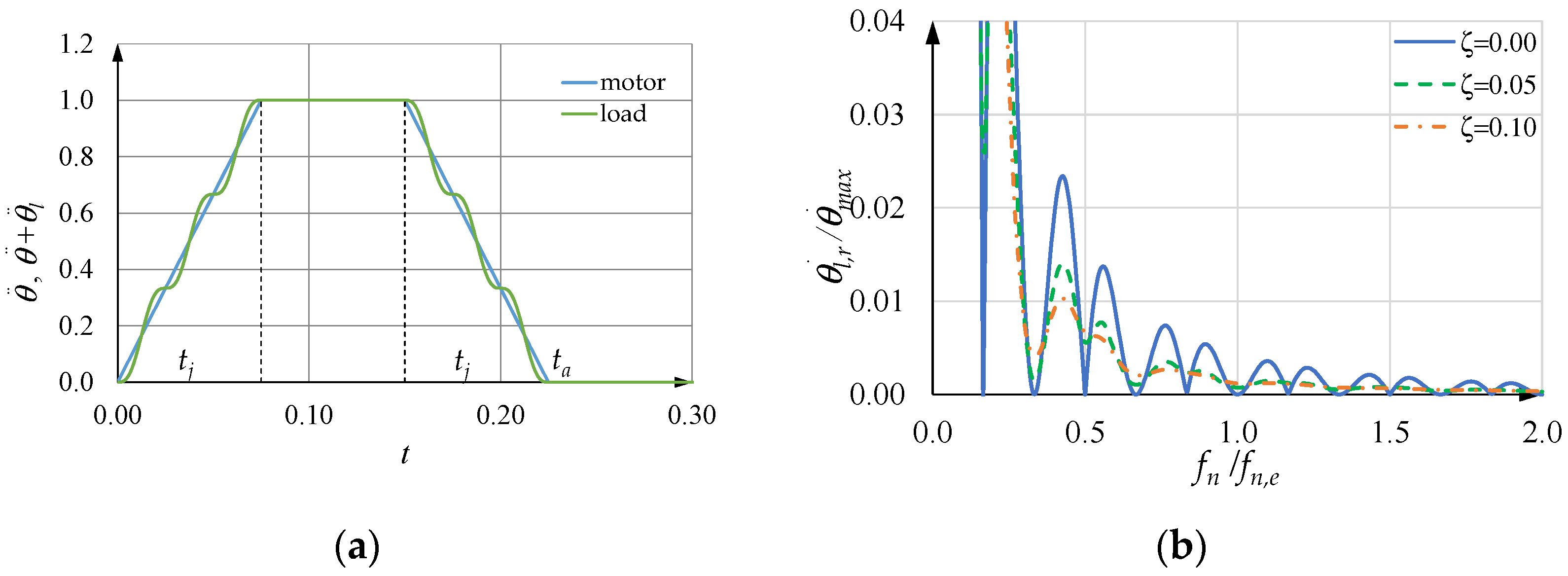
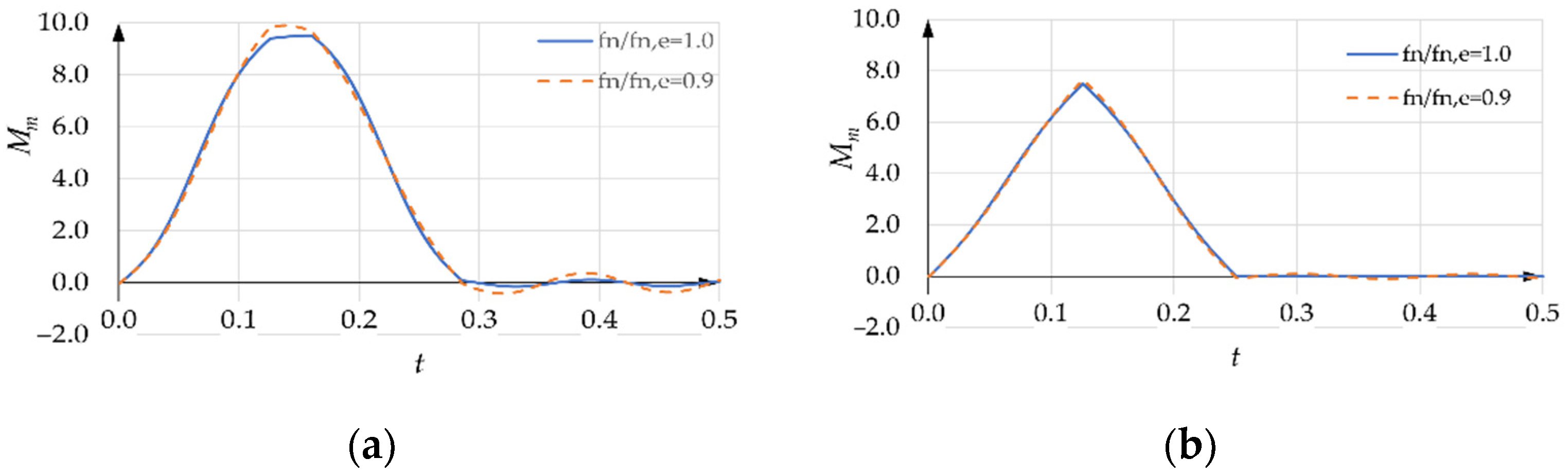
Figure 14a, Figure 15a and Figure 16a show the motor and load acceleration in the case in which ${\ddot{\vartheta }}_{Max}$ is equal to 1000.0 rad/s², ${\dot{\vartheta }}_{max}$ to 150.0 rad/s, $f_n$ to 40 Hz, when $\delta$ is equal to zero, and k_j is equal to one, two, and three, respectively. In all these cases, $t_a$ is less than $t_{a,min}$. As mentioned before, in the ramp-up time $t_{j,0,k}$, there are k_j complete oscillations of the load: an important result is that during the next time $t_c$ at constant acceleration (for the motor), the load acceleration does not show any oscillation either, but is equal to the motor acceleration. Then, during the ramp-down time $t_{j,0,k}$, there are still k_j oscillations of the load, and after time $t_a$, the load does not show any residual oscillation.

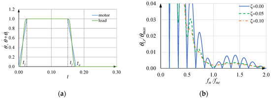
Figure 14. (a) Motor and load acceleration when $t_j=1/f_{n,e}$ and $f_n=f_{n,e}$; (b) sensitivity curve when $t_j=1/f_{n,e}$.

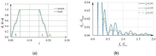
Figure 15. (a) Motor and load acceleration when $t_j=2/f_{n,e}$ and $f_n=f_{n,e}$; (b) sensitivity curve when $t_j=2/f_{n,e}$.

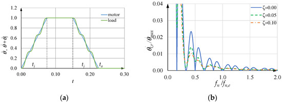
Figure 16. (a) Motor and load acceleration when $t_j=3/f_{n,e}$ and $f_n=f_{n,e}$; (b) sensitivity curve when $t_j=3/f_{n,e}$.

Figure 14b, Figure 15b and Figure 16b also show the SCs under the previous conditions when $\delta$ is equal to zero and k_j is equal to one, two, and three, respectively. They are obtained by numerical simulations, when the dimensionless structural damping coefficient $\zeta$ is equal to 0.00, 0.05 and 0.10. These figures show the following:

• Neglecting small values of $\zeta$ in the design of the acceleration profiles does not worsen the SCs; on the contrary, it improves them, even though at the estimated frequency $f_{n,e}$, there is a small residual oscillation. This behavior is general for values of $f_n{t}_a$ greater than or equal to two;
• If $t_j$ is a multiple $k_j/f_{ne}$ of the fundamental value, with k_j equal to 1, 2, …, $k_{j,max}$ (Equation (49)), the corresponding SCs are satisfactory, but a light improvement can be noticed by increasing k_j. In any case, the fundamental value $1/f_{ne}$ of $t_j$ is the minimum and thus gives the minimum value of $t_a$, and often the corresponding SC is satisfactory.

It should be noted that, when comparing the results of two acceleration profiles with different slopes but with the same time $t_a$, which is that of the greater k_j (meaning that the acceleration profile with the smaller k_j has a lower maximum acceleration), the SC generated by the profile with the greater k_j seems slightly better.

Normally, a value of $\left|{\dot{\vartheta }}_{l,r}\right|/{\dot{\vartheta }}_{max}$ of a few hundredths is admissible in velocity control.

In any case, it is interesting to note that the three SCs with $\zeta$ equal to zero in Figure 14b, Figure 15b and Figure 16b are almost overlapping in the abscissa range $\left[0.835, 1.165\right]$.

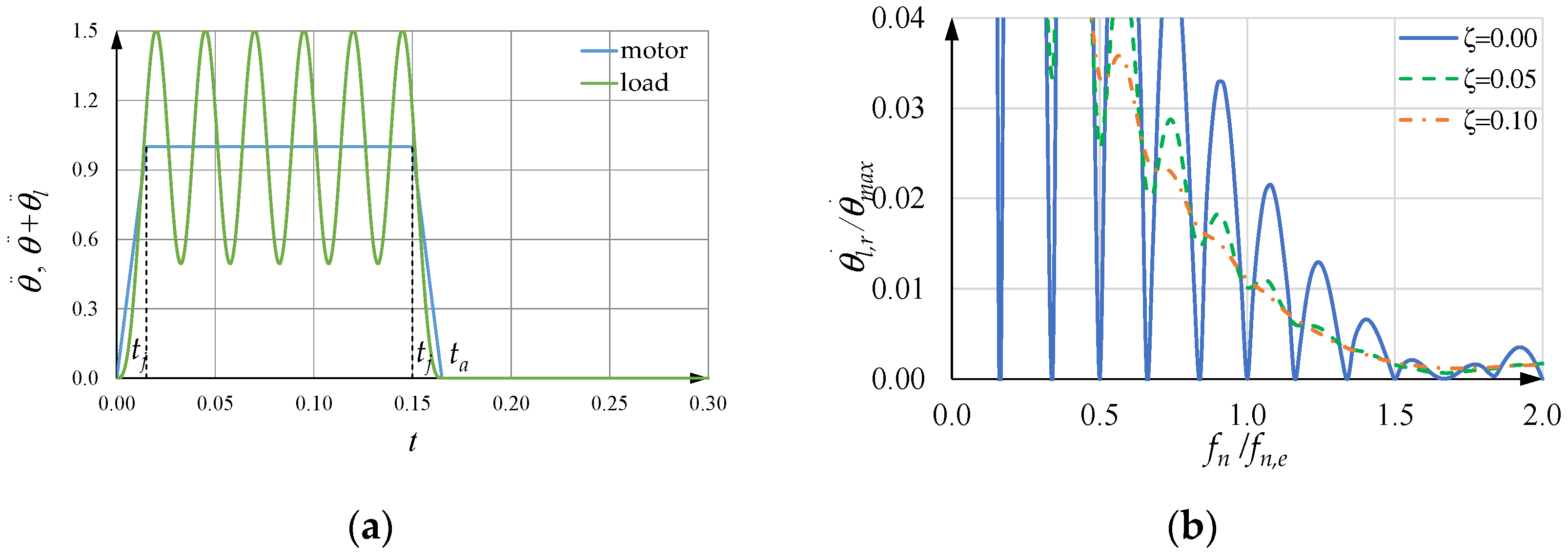
On the contrary, if $\delta$ is equal to one, particular conditions must be satisfied as is explained in Appendix C, and the SCs are not as satisfactory. For example, if $f_n{t}_{a,min}$ is an integer number, $t_a$ satisfies the inequalities in Equation (25) and $t_j$ is less than $1/f_{n,e}$, Figure 17a shows the motor and load acceleration for the same case of Figure 14a, Figure 15a and Figure 16a, but with $\delta$ equal to one, k_j equal to zero, and $t_a$ equal to 0.165 s.

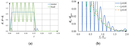
Figure 17. (a) Motor and load acceleration when $t_j=dec\left(f_{n,e}{t}_a\right)/f_{n,e}$; (b) sensitivity curve when $t_j=dec\left(f_{n,e}{t}_a\right)/f_{n,e}$.

When $\delta$ is equal to one, the number of free oscillations during time $t_j$ is not an integer, and the load acceleration is symmetrical with respect to the vertical line whose abscissa is $t_a/2$, so that after the acceleration time $t_a$, there is no residual vibration.

Nevertheless, significant oscillations of the load acceleration occur during the constant acceleration time $t_c$ of the motor. Even if the amplitude of the residual velocity vibration is zero, when $f_n$ is equal to $f_{n,e}$ and $\zeta$ is equal to zero, the corresponding SCs are unsatisfactory overall (Figure 17b). These observations can be extended to all the couples $\left(k_j,\delta \right)$ with $\delta$ equal to one. Hence, in the following, $t_j$ is assumed to be equal to a multiple k_j of its fundamental value $1/f_{n,e}$.

As explained above, ${\ddot{\vartheta }}_{Max}$ is a specification that can generate some difficulties due to the acceleration oscillations of the load during time $t_c$ in which the motor is at constant acceleration, and to those of the motor torque, which are mainly consequent to the former.

Assuming that the motor performs the STAP perfectly, $\zeta$ is equal to zero and the constant acceleration time $t_c$ is large enough to allow the load acceleration to reach its peak within $t_c$; thus, the oscillations of the load acceleration during this time have an amplitude $\left|{\ddot{\vartheta }}_{l,c}\right|$ that is given by the dimensionless expression

$$\frac{\left|{\ddot{\vartheta }}_{l,c}\right|}{{\ddot{\vartheta }}_{max}}=\frac{\sqrt{2}\sqrt{1-cos\left(2\pi \frac{f_n}{f_{ne}}{k}_j\right)}}{2\pi \frac{f_n}{f_{ne}}{k}_j}.$$

(57)

Figure 18 shows $\left|{\ddot{\vartheta }}_{l,c}\right|/{\ddot{\vartheta }}_{max}$ versus $f_n/f_{ne}$ when $k_j$ is equal to one and two. Generally, a greater value of $k_j$ results in smaller values of the ordinate. The two curves almost overlap in a small range around one.

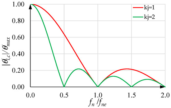
Figure 18. $\left|{\ddot{\vartheta }}_{l,c}\right|/{\ddot{\vartheta }}_{max}$ versus $f_n/f_{n,e}$ when the load acceleration reaches its peak within $t_c$, with $k_j$ equal to one and two.

If $M_{m,max}$ denotes the quantity,

$$M_{m,max}=\left(J_M+J_L\right){\ddot{\vartheta }}_{max},$$

(58)

the oscillations of the motor torque during time $t_c$ have an amplitude $\left|M_{m,c}\right|$ that is given by the dimensionless expression

$$\frac{\left|M_{m,c}\right|}{M_{m,max}}=\frac{\frac{J_L}{J_M}}{1+\frac{J_L}{J_M}}\frac{\left|{\ddot{\vartheta }}_{l,c}\right|}{{\ddot{\vartheta }}_{max}}.$$

(59)

Figure 19 shows the coefficient $\left(J_L/J_M\right)/\left(1+J_L/J_M\right)$ versus $J_L/J_M$. Normally, $J_L/J_M$ should assume values less than one, so as to limit the effect of $\left|{\ddot{\vartheta }}_{l,c}\right|/{\ddot{\vartheta }}_{max}$ on $\left|M_{m,c}\right|/M_{m,max}$.

Figure 19. $\left(J_L/J_M\right)/\left(1+J_L/J_M\right)$ versus $J_L/J_M$.

In any case, if $t_a$ is greater than $2t_{a,min}$, then ${\ddot{\vartheta }}_{max}$ is less than ${\ddot{\vartheta }}_{Max}$ and the effects of the oscillations of load acceleration and motor torque are less constraining.

The curves obtained from Equations (57) and (59) are theoretical and neglect the effects of the closed motor velocity chain. Therefore, it is necessary to be precautious.

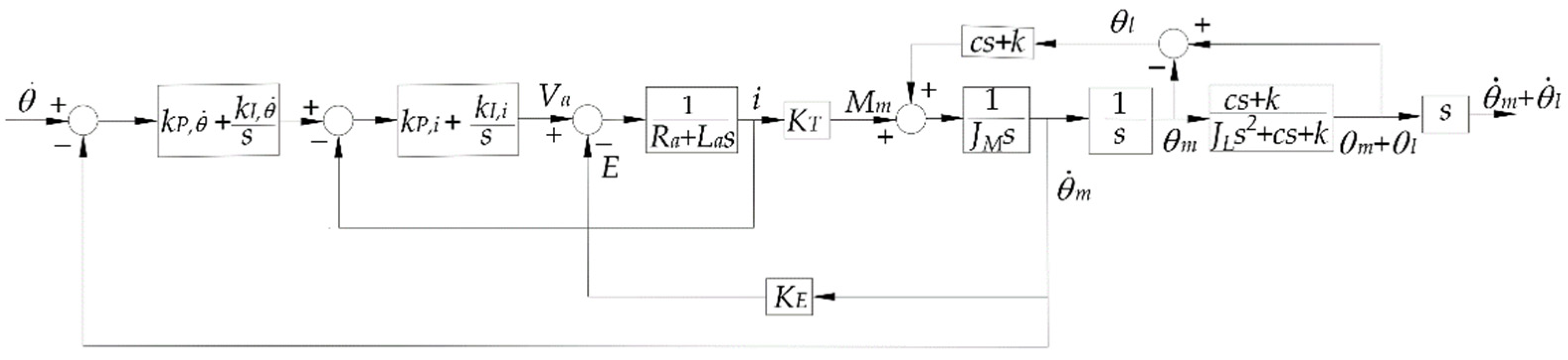
The results of numerical simulations on models with zero structural damping coefficient are shown here. A practical example is that discussed in Section 6 of [19], in which particular values of the system parameters are considered. Hereafter the motor is always the same and is controlled in a closed velocity chain, with an internal closed current chain. An essential control block diagram is shown in Figure 20. The motor characteristics are shown in Table 2. The maximum velocity ${\dot{\vartheta }}_{max}$ is equal to 150 rad/s. Two different loads are considered: the first with $J_L$ equal to $J_M$, the second with $J_L$ equal to one fourth of $J_M$. In both cases, $f_{n,e}$ is equal to 8 Hz (k changes consequently) and two frequency conditions are considered, i.e., $f_n/f_{n,e}$ equal to one and nine tenths. In any case, $t_j$ is equal 0.1250 s ($k_j$ is equal to one). The acceleration limit is initially the maximum of the nodal section (Equation (19)) and is different for the two loads. With the second load, $t_{a,min}$ is equal to 0.0938 s, the maximum acceleration is given by Equation (31), and it is not necessary to lower the acceleration limit. With the first load, $t_{a,min}$ is initially equal to 0.15 s, and the acceleration limit can be reached. Nevertheless, as can be seen from the diagrams in Figure 18 and Figure 19, $\left|M_{m,c}\right|$ is nearly equal to $0.055 M_{m,max}$, so that the acceleration limit must be lowered to 0.94 times the maximum of the nodal section to avoid exceeding $M_{m,Max}$.

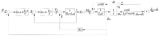
Figure 20. Control block diagram.

Table 2. Characteristics of the motor in consideration.

Resistance	Inductance	Torque Constant	Moment of Inertia	Torque Limit
Ra	La	KT = KE	JM	Mm,Max
0.9$\Omega$	0.015 H	0.8 Nm/A	0.005 kgm2	10 Nm

The following considerations can be made:

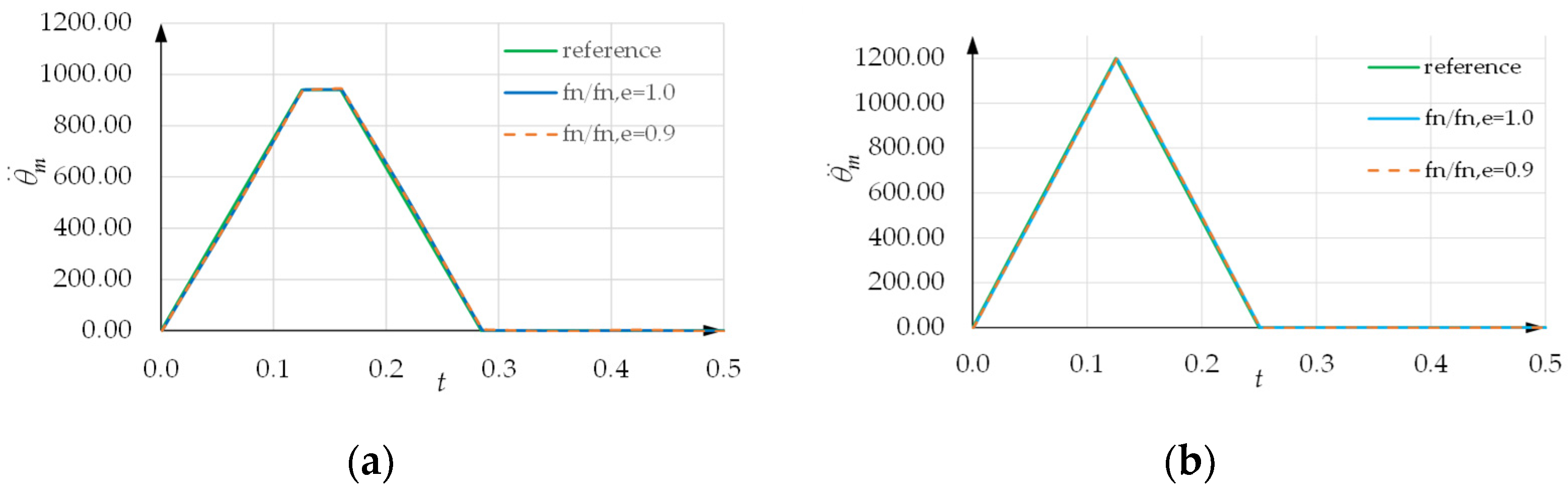
• In each case (Figure 21a,b), the motor acceleration follows the reference acceleration, i.e., the designed STAP, closely;
  

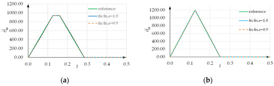  Figure 21. Motor acceleration versus time: (a) $J_L/J_M=1.00$; (b) $J_L/J_M=0.25$.
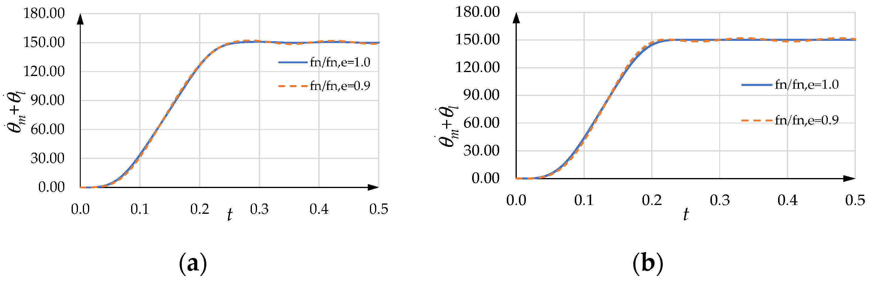
• In each case (Figure 22a,b), when $f_n$ is equal to $f_{n,e}$, the residual oscillations of the load velocity are extremely small;
  

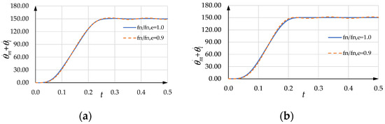  Figure 22. Load velocity versus time: (a) $J_L/J_M=1.00$; (b) $J_L/J_M=0.25$.
• In each case (Figure 22a,b), when $f_n$ is equal to nine tenths of $f_{n,e}$, the residual oscillations of the load velocity are small but tangible; they can be obtained approximately from the corresponding SCs;
• With $J_L$ equal to $J_M$ (Figure 23a), the differences in the motor torque at the two frequencies are tangible; furthermore, if $f_n$ is equal to $f_{n,e}$, the residual oscillations of the motor torque are small, while if $f_n$ is equal to nine tenths of $f_{n,e}$, they are larger;
  

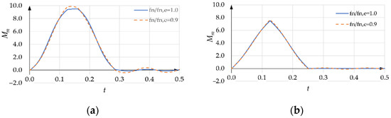  Figure 23. Motor torque versus time: (a) $J_L/J_M=1.00$; (b) $J_L/J_M=0.25$.
• With $J_L$ equal to one fourth of $J_M$ (Figure 23b), the differences in the motor torque at the two frequencies are very small; furthermore, if $f_n$ is equal to $f_{n,e}$, the residual oscillations of the motor torque are negligible, while if $f_n$ is equal to nine tenths of $f_{n,e}$, they are very small.

Other numerical simulations with a positive and very small value of $\zeta$ provide similar results.

All these numerical simulations confirm the validity of the proposed approach for the design of a STAP.

4. Discussion

Now, under the assumption that $t_j$ is a multiple k_j of the fundamental value $1/f_{n,e},$ if the maximum possible acceleration ${\ddot{\vartheta }}_{max,M}$ (Equation (31)) is reached, two cases can be distinguished:

1.

The jerk time is less than or equal to $t_{a,min}$, i.e.,

$$k_j/f_n\le t_{a,min}.$$

(60)

In this case, the acceleration limit ${\ddot{\vartheta }}_{Max}$ is reached and

$$t_a=t_{a,min}+\frac{k_j}{f_n}.$$

(61)

In dimensionless form, Equation (61) can be written as

$$\frac{t_a}{t_{a,min}}=1+\frac{k_j}{f_n{t}_{a,min}} \mathrm{with} 1<\frac{t_a}{t_{a,min}}\le 2.$$

(62)

Obviously, the values of $k_j$ for which this is possible are given by

$$k_j\le int\left(f_n{t}_{a,min}\right).$$

(63)

Furthermore, ${\stackrel{⌢}{t}}_{j,max}$ is given by

$${\stackrel{⌢}{t}}_{j,max}=\frac{k_j}{k_j+f_n{t}_{a,min}}.$$

(64)

2.

The jerk time is greater than or equal to $t_{a,min}$, i.e.,

$$k_j/f_n\ge t_{a,min}.$$

(65)

In this case, the maximum possible acceleration ${\ddot{\vartheta }}_{max,M}$ is reached with a triangular acceleration profile, such that

$$t_a=\frac{2k_j}{f_n}.$$

(66)

As a result, the ratio $t_a/t_{a,min}$ assumes the value

$$\frac{t_a}{t_{a,min}}=\frac{2k_j}{f_n{t}_{a,min}} \mathrm{with}\frac{t_a}{t_{a,min}}\ge 2.$$

(67)

Obviously, in this case, $f_n{t}_a$ is the integer number $2k_j$.

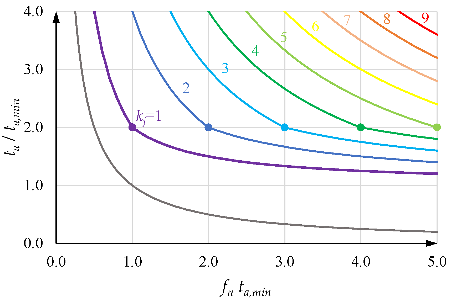
The set of two Equations (62) and (67) can be written as a single equation:

$$\frac{t_a}{t_{a,min}}=g\left(f_n{t}_{a,min};k_j\right).$$

(68)

Figure 24 shows the curves of $t_a/t_{a,min}$ as functions of $f_n{t}_{a,min}$, with k_j as a parameter. These curves can also be interpreted as lower limits, because, for a given abscissa $f_n{t}_{a,min}$, they give the minimum possible value of $t_a/t_{a,min}$ and thus of $t_a$ when $t_j$ is equal to a multiple of its fundamental value. Obviously, it is possible to choose a greater value of $t_a/t_{a,min}$. In this case, the acceleration time is greater and the maximum acceleration is less.

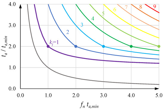
Figure 24. Curves showing the minimum value of $t_a/t_{a,min}$ versus $f_n{t}_{a,min}$ when $t_j$ is equal to $k_j/f_n$.

The minimum value of $t_a$ depends on the natural frequency $f_n$. The curves are monotonously decreasing. The analysis of what happens if $f_n$ changes for a given $t_{a,min}$ shows that if $f_n$ is high enough, a smaller value of $t_a/t_{a,min}$, i.e., a shorter acceleration time, can be adopted. On the contrary, for low values of $f_n$, the acceleration time must be high enough and the acceleration limit ${\ddot{\vartheta }}_{Max}$ cannot be reached.

The inequality

$$\frac{t_a}{t_{a,min}}\ge g\left(f_n{t}_{a,min};k_j\right)$$

(69)

can also be read as

$$f_n{t}_{a,min}\ge \stackrel{\sim }{g}\left(\frac{t_a}{t_{a,min}};k_j\right),$$

(70)

where $\stackrel{\sim }{g}$ is the inverse function of g. This means that, for each value of $t_a$ and $t_{a,min}$, there exists a minimum value of $f_n$, such that, with a given acceleration time $t_a$, a STAP allows the load to have zero residual oscillations and a sufficiently satisfactory SC.

For the sake of completeness, it should be noted that, irrespective of the acceleration limit ${\ddot{\vartheta }}_{Max}$ and thus of $t_{a,min}$, there is no STAP capable of reaching velocity ${\dot{\vartheta }}_{max}$ with zero residual vibration of the load velocity if

$$f_n{t}_a<1,$$

(71)

i.e., in each case, the acceleration time $t_a$ must satisfy

$$t_a\ge \frac{1}{f_n}.$$

(72)

In order to represent this inequality in Figure 23 (the brown curve), the two terms are made dimensionless with reference to $t_{a,min}$, i.e.,

$$\frac{t_a}{t_{a,min}}\ge \frac{1}{f_n{t}_{a,min}}.$$

(73)

To minimize the settling time of the load velocity, the normal procedure is to assume the jerk time equal to one, or at most two, estimated periods of the undamped free oscillations and the acceleration time depending on whether $t_a$ is less or greater than $2t_{a,min}$, and to evaluate the corresponding SC. Therefore, it is convenient to start from the fundamental value $t_{j,0,1}$, and, in brief:

1.

If

$$f_{n,e}{t}_{a,min}\ge 1,$$

(74)

it is possible to adopt a STAP that reaches the acceleration limit ${\ddot{\vartheta }}_{Max}$, at least with the fundamental value $t_{j,0,1}$. This allows $t_a$ to assume its minimum value and, simultaneously, there is no residual velocity oscillation if $f_n$ is equal to its estimated value. Furthermore, the corresponding SC is satisfactory, especially if $f_{n,e}{t}_a$ is sufficiently high.

Furthermore, if

$$f_{n,e}{t}_{a,min}\gg 1,$$

(75)

it is possible to adopt a multiple value of the fundamental value $t_{j,0,1}$, with a small increase in $t_a$, but with a qualitative improvement of the corresponding SC, if this improvement is worthy of consideration.

2.

Otherwise, if

$$f_{n,e}{t}_{a,min}<1,$$

(76)

it is not possible to adopt a STAP that reaches the acceleration limit ${\ddot{\vartheta }}_{Max}$. Instead, it is possible to go from a triangular profile, in which $t_a$ assumes its minimum value equal to $2/f_{n,e}$, to STAPs with greater values of $t_a$ to have a better SC. Since the inequality in Equation (76) is often verified at low values of $f_{n,e}$, the increase in $t_a$ in the transition from the fundamental value $t_{j,0,1}$ to the next can be significant.

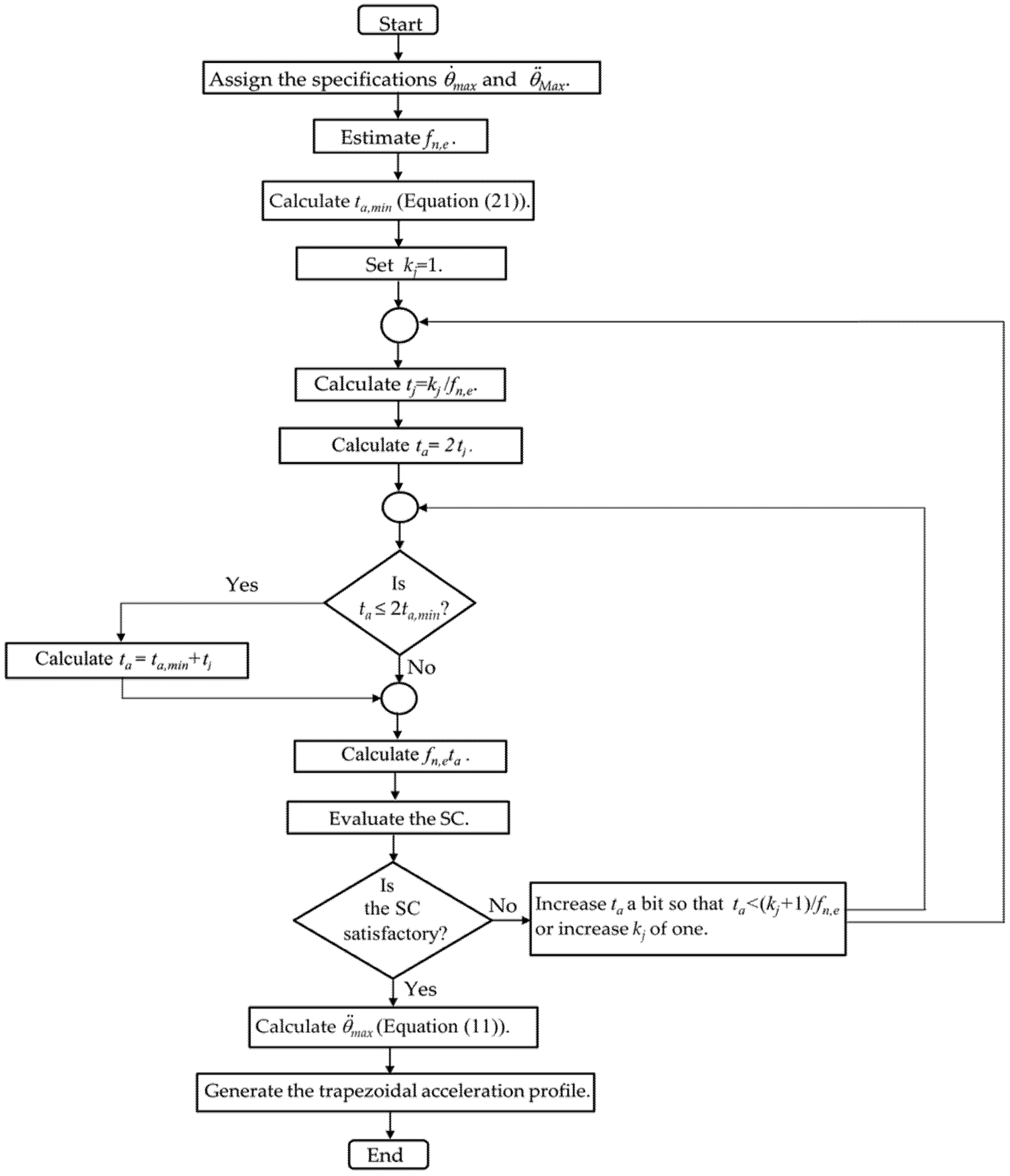
Figure 25 shows the flowchart of the design procedure of the motor STAP. For simplicity, ${\ddot{\vartheta }}_{Max}$ is assigned as a specification from the beginning and no longer changed.

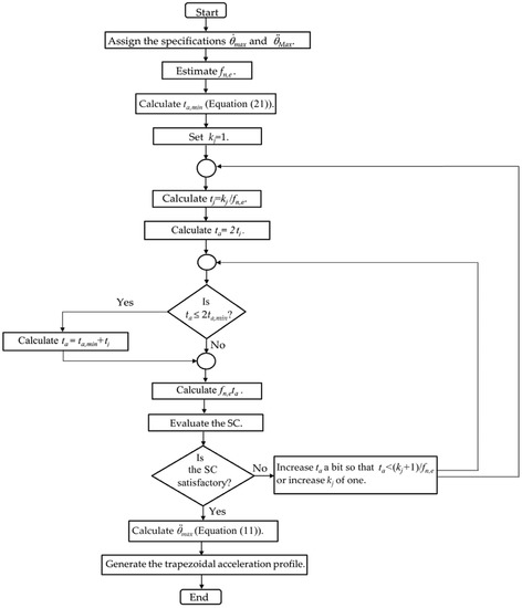
Figure 25. Flowchart of the procedure to design the STAP of the motor.

5. Conclusions

The present paper concerns a rest-to-velocity motion. It considers trapezoidal acceleration profiles, which are widely used in applications involving oscillating systems, with the aim of designing them so as to have the motor motion in a minimum acceleration time and limited residual load vibrations.

This paper draws inspiration from [20], in comparison to which, however, it

• Makes the time dimensionless with respect to the acceleration time. This implies that it is possible to have simple analytical expressions of the jerk time that prevent the load from having residual oscillations;
• Broadens the analysis to acceleration times much greater than twice the minimum value imposed by the motor’s acceleration limit. This broadening is necessary to allow the designer to deal with natural frequencies that would otherwise be excluded from the analysis;
• Sets the limits of the acceleration time imposed by the natural frequency, indicating the minimum value that this time can reach in each application;
• Highlights the characteristics of the load acceleration profile at the estimated frequency $f_{n,e}$;
• Analyzes the sensitivity curves of velocity, and thus the range of natural frequencies, around the estimated one, in which the residual vibrations of the load can be considered sufficiently small;
• Compares the different solutions corresponding to multiples of the fundamental value of the jerk time;
• Shows a procedure, explained in a flowchart, with which to design a trapezoidal acceleration profile for a rest-to-velocity motion.

Ultimately, this work provides a comprehensive overview of the design of a STAP by relating all the most significant parameters: ${\dot{\vartheta }}_{max}$, ${\ddot{\vartheta }}_{Max}$, $t_a$, $t_{a,min}$, $t_j$, $f_{n,e}$, and $J_L/J_M$.

To optimize the settling time of the load velocity, the jerk time is normally chosen to be equal to one, or at most two, estimated periods of the undamped free oscillations and the acceleration time according to two different rules, depending on whether $t_a$ is less or greater that $2t_{a,min}$, and to the evaluation of the corresponding sensitive curve.

Numerical simulations on a complete system, with the motor controlled in a closed chain and a zero or very small structural damping coefficient, confirm that the proposed acceleration profiles allow the motor to have a minimum acceleration time and the load a satisfactory settling time.

A future paper, of which the present one is preparatory, will deal with the optimization of the load settling time in a point-to-point motion.

References

- Singer, N.C.; Seering, W.P. Preshaping command inputs to reduce system vibration. J. Dyn. Syst. Meas. Control Trans. ASME 1990, 112, 76–82. [Google Scholar] [CrossRef]
- Dwivedy, S.K.; Eberhard, P. Dynamic analysis of flexible manipulators, a literature review. Mech. Mach. Theory 2006, 41, 749–777. [Google Scholar] [CrossRef]
- Singhose, W. Command shaping for flexible systems: A review of the first 50 years. Int. J. Precis. Eng. Man. 2009, 4, 153–168. [Google Scholar] [CrossRef]
- Rashidifar, M.A.; Ahmadi, D.; Rashidifar, A.A. Optimal input shaping for vibration control of a flexible manipulator using genetic algorithm. Adv. Mech. Eng. Appl. 2012, 2, 141–152. [Google Scholar]
- Huang, J.; Liang, Z.; Zang, Q. Dynamics and swing control of double-pendulum bridge cranes with distributed-mass beams. Mech. Syst. Sig. Process. 2015, 54–55, 357–366. [Google Scholar] [CrossRef]
- Kotate, S.; Yagi, K.; Takigami, T. Application of sampled-data control by using vibration manipulation function to suppress residual vibration of travelling crane. JSME Mech. Eng. J. 2015, 2, 15-00033. [Google Scholar]
- Alghanim, K.A.; Alhazza, K.A.; Masoud, Z.N. Discrete-time command profile for simultaneous travel and hoist maneuvers of overhead cranes. J. Sound Vib. 2015, 345, 47–57. [Google Scholar] [CrossRef]
- Mar, R.; Goyal, A.; Nguyen, V.; Yang, T.; Singhose, W. Combined input shaping and feedback control for double-pendulum systems. Mech. Syst. Sig. Process. 2017, 85, 267–277. [Google Scholar] [CrossRef]
- Fujoka, D.; Singhose, W. Optimized input-shaped model reference control on double-pendulum system. J. Dyn. Syst. Meas. Control Trans. ASME 2018, 140, 101004. [Google Scholar] [CrossRef]
- Maghsoudi, M.J.; Nacer, H.; Tocki, M.O.; Mohamed, Z. A novel approach in S-shaped input design for higher vibration reduction. Appl. Model. Simul. 2018, 2, 76–83. [Google Scholar]
- Ichikawa, S.; Castro, A.; Johnson, N.; Kojima, H.; Singhose, W. Dynamics and command shaping control of quadcopters carrying suspended loads. IFAC PapersOnLine 2018, 51, 84–88. [Google Scholar] [CrossRef]
- Hou, Z.; Geng, Y.; Huang, S. Minimum residual vibrations for flexible satellites with frequency uncertainty. IEEE Trans. Aerosp. Electron. Syst. 2018, 54, 1029–1038. [Google Scholar] [CrossRef]
- Sharma, A.K. Design of command-shaping scheme for mitigating residual vibrations in dielectric elastomer actuators. J. Appl. Mech. 2019, 87, 021007. [Google Scholar] [CrossRef]
- Newmann, M.; Lu, K.; Khoshdarregi, M. Suppression of robot vibrations using input shaping and learning-based structural models. J. Intel. Mat. Syst. Str. 2021, 32, 1001–1012. [Google Scholar] [CrossRef]
- Alhazza, K.A.; Masoud, Z.N.; Alqabandi, J.A. A close-form command shaping control for point-to-point maneuver with nonzero initial and final conditions. Mech. Syst. Signal Process. 2022, 170, 108804. [Google Scholar] [CrossRef]
- Hoshyari, S.; Xu, H.; Knoop, E.; Coros, S.; Bächer, M. Vibration-minimizing motion retargeting for robotic characters. ACM Trans. Graph. 2019, 38, 1–14. [Google Scholar] [CrossRef]
- Shah, M.A.; Lee, D.G.; Lee, B.Y.; Kim, N.W.; An, H.; Hur, S. Actuating voltage waveform optimization of piezoelectric inkjet printhead for suppression of residual vibrations. Micromachines 2020, 11, 900. [Google Scholar] [CrossRef] [PubMed]
- Ha, C.W.; Rew, K.H.; Kim, K.S. Robust zero placement for motion control of lightly damped systems. IEEE Trans. Ind. Electron. 2013, 60, 3857–3864. [Google Scholar] [CrossRef]
- Yoon, H.J.; Chung, S.Y.; Kang, H.S.; Hwang, M.J. Trapezoidal motion profile to suppress vibration of flexible object moved by robot. Electronics 2019, 8, 30. [Google Scholar] [CrossRef] [Green Version]
- Meckl, P.H.; Arestides, P.B. Optimized S-curve motion profiles for minimum residual vibration. In Proceedings of the 1998 American Control Conference, Philadelphia, PA, USA, 26–26 June 1998; IEEE Cat. No.98CH36207. Volume 5, pp. 2627–2631. [Google Scholar]
Publisher’s Note: MDPI stays neutral with regard to jurisdictional claims in published maps and institutional affiliations. |
© 2022 by the author. Licensee MDPI, Basel, Switzerland. This article is an open access article distributed under the terms and conditions of the Creative Commons Attribution (CC BY) license (https://creativecommons.org/licenses/by/4.0/).