A Multi-Factor Driven Model for Locomotive Axle Temperature Prediction Based on Multi-Stage Feature Engineering and Deep Learning Framework

Abstract

Recently, with the increasing scale of the volume of freight transport and the number of passengers, the study of railway vehicle fault diagnosis and condition management is becoming more significant than ever. The axle temperature plays a significant role in the locomotive operating condition assessment that sudden temperature changes may lead to potential accidents. To realize accurate real-time condition monitoring and fault diagnosis, a new multi-data-driven model based on reinforcement learning and deep learning is proposed in this paper. The whole modeling process contains three steps: In step 1, the feature crossing and reinforcement learning methods are applied to select the suitable features that could efficiently shorten the redundancy of the input. In step 2, the stack denoising autoencoder is employed to extract deep fluctuation information in the features after the reinforcement learning. In step 3, the bidirectional gated recurrent unit algorithm is utilized to accomplish the forecasting model and achieve the final results. These parts of the integrated modeling structure contributed to increased forecasting accuracy than single models. By analyzing the forecasting results of three different data series, it could be summarized that: (1) The proposed two-stage feature selection method and feature extraction method could greatly optimize the input for the predictor and form the optimal axle temperature forecasting model. (2) The proposed hybrid model can achieve satisfactory forecasting results which are better than the contrast algorithms proposed by other researchers.

1. Introduction

Due to the huge demands of passenger and freight transport on the railway currently, a mass of transportation tasks are taken by locomotives as one of the main transport capacities of railway, leading to quite frequent operations [1]. However, fast speeds and long mileage have also brought greater challenges to the reliability and efficiency of railway engineering [2]. The axle situation of the bogies is an essential indicator to reflect the real-time monitoring of vehicle transportation safety. The abnormal thermal wave changes of the axles may lead to potential accidents, such as cut axle, hot axle, or even train derailment [3]. Therefore, axle temperature forecasting is of great value for real-time monitoring and alarm equipment in the operation and maintenance strategy [4]. The vehicle data transmitted by the onboard sensors should be deeply analyzed for the changing trend of the locomotive data and further drive decision-making [5]. Vale et al. used various sensor data on board in failure detection for early warnings [6]. Liu proposed a new monitoring system based on onboard switched Ethernet for the fault diagnosis [7]. Bin et al. constructed a non-destructive embedding detecting system for axle temperature compensation [8]. The above-proposed methods could achieve real-time data measuring of railway vehicles, but accurate forecasting and the detailed analysis of internal correlations in railway vehicles are still required precautions to avoid supernumerary vehicle maintenance. Recently, scholars have developed many forecasting models in the field of temperature prediction [9], wind speed prediction [10], power prediction [11], traffic flow prediction [12], air pollutant forecasting [13], etc. Therefore, it is indispensable to establish prediction models for the changing trend of the axle temperature, to obtain early warning and fault diagnosis of the faulty position of the axle in advance to prevent major accidents. Therefore, the forecasting models of railway vehicle status with positive performance are worth studying.

1.1. Related Work

In recent years, scholars have excogitated plenty of effective prediction methods in the research aspects of railway vehicle fault diagnosis. Mainstream forecasting models include statistical models, physical models, and artificial intelligence (AI) models [14]. The physical method mainly predicts the thermal analysis based on the mechanical properties of the materials on each component for the axle system through physical modeling methods, such as finite element analysis [15]. Statistical methods mainly use regression modeling methods to realize the forecasting process by analyzing the historical railway vehicle data of various influence factors. For example, the stepwise regression analysis was employed to predict the axle temperature data collected by sensors in high-speed trains, which transmitted the raw temperature data into the regression equation with other relevant factors [16].

The above two kinds of method still require stable time series data and may present difficulty in information extraction. However, under non-uniform speeds, the onboard system of the trains will collect the original non-stationary axle temperature. On the contrary, the AI methods could establish nonlinear models by analyzing the deep information of raw data [17]. Therefore, scholars have proposed various artificial intelligence algorithms to establish accurate and effective forecasting models for further improvement. Liu applied the backpropagation neural network (BPNN) to predict trains’ axle temperatures and exceed GM (1, 1) with better accuracy [18]. Abdusamad proposed multiple linear regression (MLR) in future temperature forecasting [19]. Xiao et al. conducted experiments on output shaft gearbox temperature forecasting by the least-square support-vector machine (LSSVM) [20].

As an important part of artificial neural networks, the deep learning algorithm is widely applied. Fu et al. designed a new modeling structure to analyze the gearbox-bearing temperature changes by the convolutional neural network (CNN) and the long short-term memory (LSTM) [21]. Yang et al. used a new modeling structure to analyze temperature changes during high-speed train operation using the LSTM model, which showed that the forecasting errors were arranged within a reasonable range [22]. The gated recurrent unit (GRU) is also employed for bearing residual life forecasting [23]. The GRU network obtained the best results against other algorithms.

Despite their frequent application in time-series research, single prediction algorithms have difficulty in analyzing complicated irregular datasets. The hybrid methods can integrate artificial neural methods and data processing methods to get higher prediction accuracy than single predictors. Therefore, the feature extraction and feature selection approaches are proposed to optimize the input features for the deep learning predictors and improve model performance dramatically [24]. The feature extraction algorithms could analyze the implicit data information and improve the input quality for the predictor. Chen et al. applied the principal component analysis (PCA) to optimize the input of the radial basis function neural network (RBFNN) [25]. Khan et al. also chose the PCA to extract the hidden features in the original data and reduce the dimension [26]. Jaseena and Kovoor presented the stacked autoencoder (SAE) to obtain considerable features from the raw data, which have greatly improved the results in the LSTM network [27]. Furthermore, Rizwan’s group established a novel power prediction model combining the stacked denoising autoencoder (SDAE) and SVM, which proved the validity of SDAE in a hybrid framework [28].

The feature selection methods are advantageous to reduce data redundancy and overfitting problems [29]. An efficient feature selection process should be conducted by the actual data characteristics and could obtain a compact and relevant feature subset to improve model accuracy and reduce time costs [30]. To analyze the influencing factors in fault diagnosis, feature crossing (FC) validation could estimate the effect of the modeling function on the raw datasets to select the proper parameters [31]. The common feature selection algorithms are mainly heuristic algorithms. Ant colony optimization (ACO) is a probabilistic and approximation heuristic method to realize complex optimization. Paniri et al. designed a framework of ACO in ensemble feature selection, which acquires from experiences, based on the temporal difference (TD) algorithm [32]. For the multi-label learning processes based on datasets, a multi-label feature selection method based on ant colony optimization (MLACO) is also proposed to obtain the best features with less redundancy and better relevancy, which can be applied in different aspects [33]. Hashemi et al. also constructed an ACO algorithm using a multi-criteria decision-making (MCDM) process to select the most relevant features for complex optimization [34]. Another filter feature selection method for multi-label learning, which is the multi-label feature selection using multi-criteria decision making (MFS-MCDM), could analyze the features based on their correlation with multiple labels in the information fusion process [35]. Zhang et al. used the fruit fly optimization (FFO) algorithm in the feature selection approach to enhance the echo state network (ESN) predictor and obtained satisfying outputs [36]. Zheng et al. selected the features using the particle swarm optimization and gravitational search algorithm (PSOGSA) for predictors [37]. Bayati et al. developed a memetic-based sparse subspace learning (MSSL) algorithm for multi-label classification that could select high-quality features and delete redundant features [38]. Hashemi et al. applied a fast algorithm for feature selection on the multi-label data with the PageRank algorithm, which is called multi-label graph-based feature selection (MGFS) [39]. The effectiveness of the proposed model in the classification criteria and run-time has been proved by the experiment results. The abovementioned algorithms have been applied in prediction and improved to some extent. For more achievement in the modeling, reinforcement learning is taken into consideration by scholars. Feng et al. applied Q-learning as the modeling selectors, which presented adaptive ability and obtained the best result with the highest accuracy [40]. Xu et al. also chose Q-learning in feature selection to raise the modeling and outperformed other heuristic algorithms [41].

From the above literature investigation, the integrated modeling algorithms could eliminate the errors and optimize the hybrid frameworks. The following points can be given: (1) As the key parts of hybrid frameworks, the complex learning structure in the deep learning methods may increase the nonlinear fitting ability. (2) The feature selection based on reinforcement learning is employed to evaluate the effect and relevancy of the features for data optimization. With the FC validation, the feature selection results could be more accurate with minimal errors. As a consequence, it is very important to choose the appropriate feature selection methods for modeling improvement. (3) The feature extract methods could obtain useful information and alleviate the noise of the input vector. Therefore, the study applies SDAE to improve the selected input features for the deep learning predictors after the hybrid feature selection.

1.2. Novelty of the Study

From the related works and literature research results, a multi-data-driven axle temperature prediction framework based on reinforcement learning and deep learning is presented in this paper. The main innovations and contributions of the study are shown as follows:

(1)

In the study, a new locomotive axle temperature forecasting model is constructed on the locomotive status to comprehensively analyze multi-data and improve the prediction accuracy of the time series framework.

(2)

A new two-stage feature selection method is designed in the paper. The feature crossing can search for useful features and evaluate the deep information of the datasets. The reinforcement learning algorithm is applied to select the optimal feature to ensure data quality. The hybrid two-stage feature selection structure is firstly utilized in locomotive axle temperature forecasting.

(3)

The stacked denoising autoencoder is used as the feature extraction approach to obtain the primary features and detailed information of the preprocessed data as the input of the bidirectional gated recurrent unit (BIGRU). For the favorable forecasting performance of deep learning, the model is firstly applied in the locomotive axle temperature prediction model as the core predictor to obtain the final result.

(4)

The multi-data-driven model FC-Q-SDAE-BIGRU adopted in the article is a new structure. To prove the high-precision performance of the presented axle temperature forecasting model, other alternative models were reproduced and tested with the proposed model.

2. Methodology

In this section, the main methodologies applied in the proposed model will be explained in the following subsections, which are the whole framework, the two-stage feature selection, the feature extraction methods, and the deep learning algorithm.

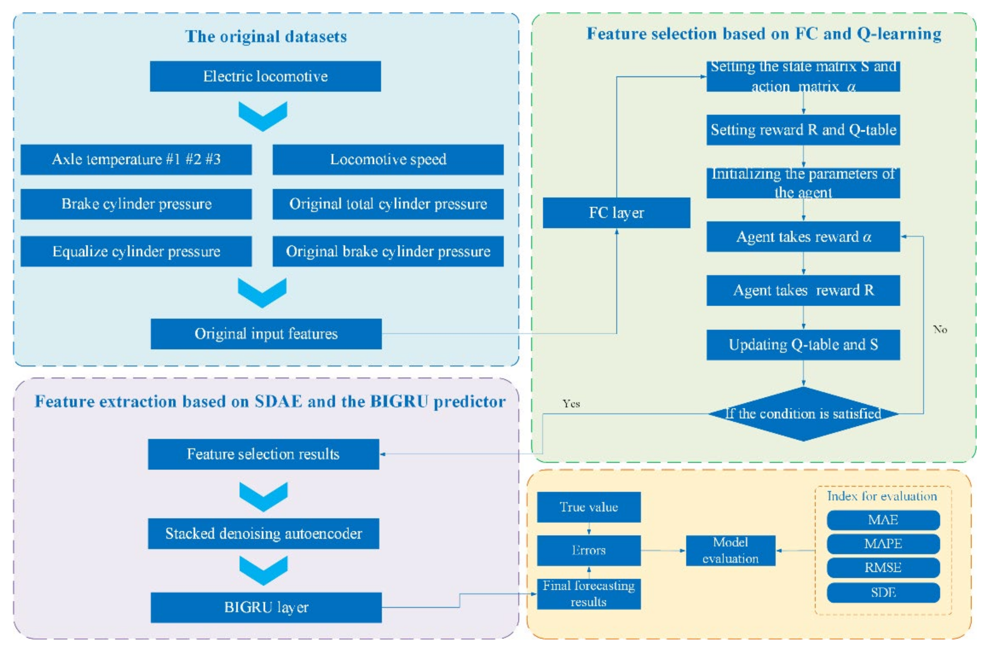
2.1. The Framework of the Proposed Model

Considering the dynamic influencing factors on locomotive axle temperature, the forecasting accuracy of simple data series should be further optimized to fulfill the application of vehicle status control. The paper presents a multi-data-driven model, which contains feature extraction, two-stage feature selection, and deep learning methods. The structure of the proposed model is dispalyed in Figure 1. Eight raw datasets, including historical datasets of three-axle temperature datasets, locomotive speeds, original total cylinder pressures, equalize cylinder pressures, original brake cylinder pressures, and brake cylinder pressures, are applied to establish locomotive axle temperature forecasting. The original axle temperature datasets are divided into training sets, validation sets, and testing sets. A two-step feature selection method is utilized to achieve the features that are rewarding to the forecasting, in which the feature crossing is used to avoid the loss of useful information and reinforcement learning can be applied to select optimal input features for prediction. To further reduce the nonlinearity of the datasets, SDAE was used to extract plenty of input features. The input features after feature selection and feature extraction will be transmitted into the BIGRU network to form the final forecasting for the result. The applied methods will be introduced in the following sections.

2.2. Two-Stage Feature Selection Methods

The feature selection methods in the research can be divided into two steps. The first step is feature crossing, which could extend the feature structure and provide more options for feature selection. The second step is Q-learning, which selects suitable features for the following process.

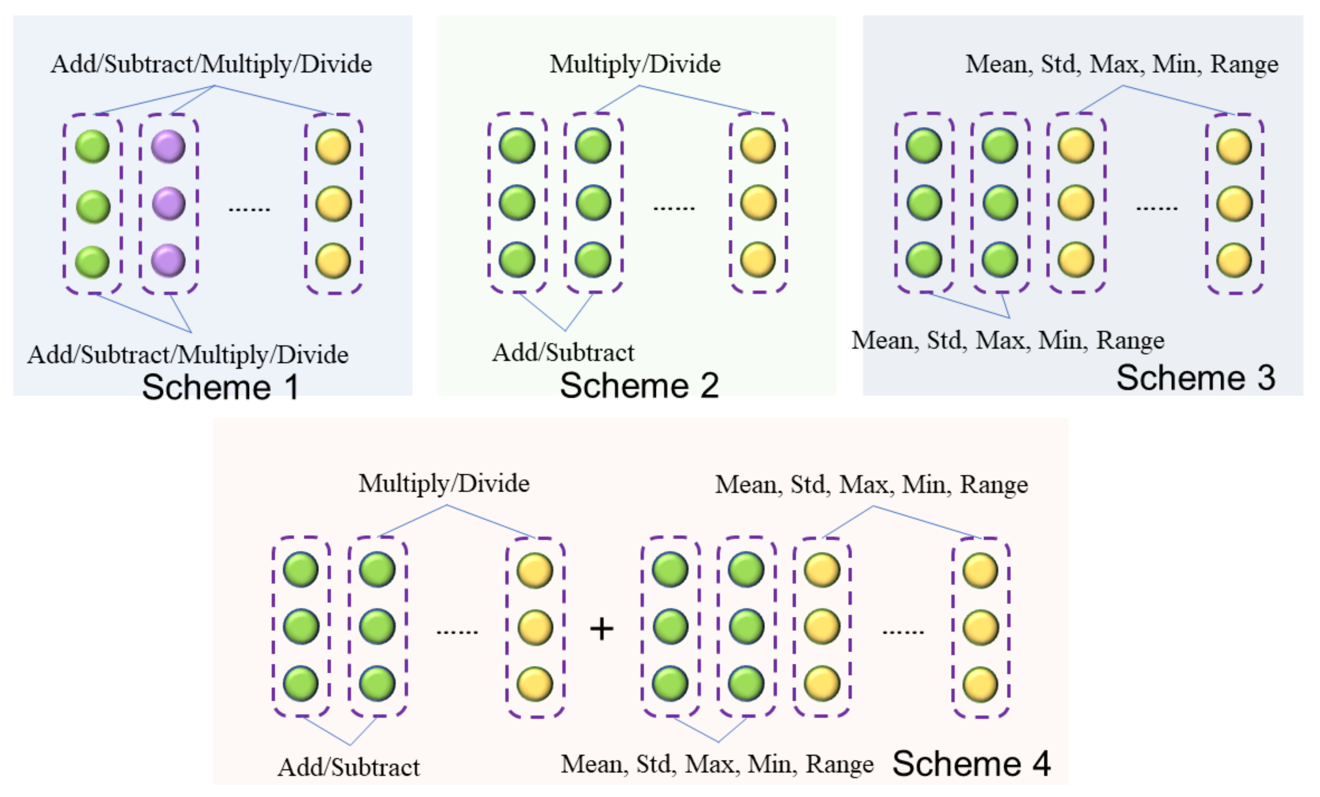
2.2.1. Stage I: Feature Crossing

A feature crossing is an integrated feature created by multiplying two or more features so that the integrations of features can possess predictive abilities beyond the single features [42]. A composite feature is generated by combining separate feature series, which contributes to establishing nonlinear connections of the data [43]. The initial features applied in the preprocessing are divided based on different domains. The degree of correlation of features from the locomotive system inside and between groups is different, considering the different contained amounts of beneficial information. The application of direct feature selection may lead to information loss, and the data then cannot be fully analyzed [44]. Therefore, feature crossing can be applied in the research. The application of feature crossing can effectively extract different information features contained in the collected data in experiments, thereby improving the performance of feature selection and strengthening the model learning ability of complex nonlinear features. In this section, four feature crossing schemes are proposed. Depending on the categories of the features, various statistical aggregations or simple calculation methods are performed on the features to obtain new features. As shown in Figure 2, the feature classes are distinguished by the colors, and the definite steps are presented as below:

Scheme 1 (FC1): Traverse the features so that the features of data preprocessing can be added, subtracted, multiplied, and divided.

Scheme 2 (FC2): Within-group features. If the two sets of features can be classified as the same class, each pair of features can be added or subtracted or otherwise, multiplied or divided.

Scheme 3 (FC3): Group aggregation features. For all the features in the same class, the mean value, standard deviation, maximum value, minimum value, and range could be calculated to obtain new features.

Scheme 4 (FC4): Within-group + group-aggregated features. The new features are integrated by Schemes 2 and 3.

The original datasets are preprocessed as input features, in which the time-series: locomotive speeds (LS), original total cylinder pressures (OTCP), equalize cylinder pressures (ECP), original brake cylinder pressures (OBCP), brake cylinder pressures (BCP), and axle temperatures (AT) are listed into five column vector features. The features generated by feature crossing may be enhanced and the invalid information may be generated so that the feature selection algorithm is used for further optimization. However, different feature crossing methods could enrich the feature structure and provide a basis for feature selection. The above four schemes are all applied in the research, then all the results and the original features are utilized in the feature selection process by the reinforcement learning algorithm. The

Table A1. Partial feature selection results of RL based on feature crossing frameworks for input features.

Datasets	Partial FC Calculation	T-5	T-4	T-3	T-2	T-1
	LS-LS1-FC1	0	0	0	0	-
	LS-OTCP1-FC1	0	0	0	1	0
#1	LS-BCP1-FC1	0	0	0	0	0
	LS-AT1-FC1	0	0	0	0	0
	LS-LS1-FC2	0	0	0	0	-
	LS-OTCP1-FC2	0	0	0	0	0
	LS-BCP1-FC2	0	0	0	0	0
	LS-AT1-FC2	0	0	1	0	0
	LS-LS1-FC3	0	0	0	0	-
	OTCP-OTCP1-FC3	0	0	0	0	-
	BCP-BCP1-FC3	1	0	0	0	-
	AT-AT1-FC3	0	0	0	0	-
	LS-LS1-FC4	0	0	0	0	-
	OTCP-OTCP1-FC4	0	0	0	0	-
	BCP-BCP1-FC4	0	0	0	1	-
	AT-AT1-FC4	0	0	0	0	-
#2	LS-LS2-FC1	0	0	0	-	0
	LS-OTCP2-FC1	0	0	0	0	0
	LS-BCP2-FC1	0	0	1	0	0
	LS-AT2-FC1	0	0	0	0	0
	LS-LS2-FC2	0	0	0	-	0
	LS-OTCP2-FC2	0	0	0	0	0
	LS-BCP2-FC2	0	0	0	0	0
	AT-AT2-FC2	1	0	0	0	0
	LS-LS2-FC3	0	0	0	-	0
	OTCP-OTCP2-FC3	0	0	0	-	0
	BCP-BCP2-FC3	0	0	0	-	1
	AT-AT2-FC3	0	0	0	-	0
	LS-LS2-FC4	0	0	0	-	0
	OTCP-OTCP2-FC4	0	0	0	-	0
	BCP-BCP2-FC4	0	0	0	-	0
	AT-AT2-FC4	0	0	1	-	0
#3	LS-LS3-FC1	0	0	-	0	0
	LS-OTCP3-FC1	0	1	0	0	0
	LS-BCP1-FC1	0	0	0	0	0
	LS-AT1-FC1	0	0	0	0	0
	LS-LS3-FC2	0	0	-	0	0
	LS-OTCP3-FC2	0	0	0	0	0
	LS-BCP3-FC2	0	0	0	0	0
	LS-AT3-FC2	0	0	0	1	0
	LS-LS3-FC3	0	0	-	0	0
	OTCP-OTCP3-FC3	0	0	-	0	0
	BCP-BCP3-FC3	0	0	-	0	0
	AT-AT3-FC3	0	0	-	0	1
	LS-LS3-FC4	0	0	-	0	0
	OTCP-OTCP3-FC4	0	0	-	0	0
	BCP-BCP3-FC4	1	0	-	0	0
	AT-AT3-FC4	0	0	-	0	0

in Appendix A lists partial feature selection results from the four scheme frameworks, in which only a small part of the results of reinforcement learning are presented due to article space limitations.

2.2.2. Stage II: Feature Selection by Reinforcement Learning

Reinforcement learning (RL) is an agent-based optimization algorithm, which can be applied to analyze and settle problems on optimal agent feedback, or to achieve satisfactory outputs through excellent learning strategies [45]. The feature selection method, which can be divided into filtering methods and bagging methods, could eliminate the redundancy of input features and further raise the modeling capability [46]. Different from the traditional evolutionary algorithms, the deep RL could achieve a positive application value in decision-making and dynamic optimization in feature extraction [47]. In the research, a feature selection method using reinforcement of the learning-based bagging method is adopted to accurately select the features. Therefore, the selection process could avoid over-fitting of the model and optimize the accuracy of the following BIRGU network. The pseudocode of Q-learning is listed in Algorithm 1 and the main calculation steps are demonstrated below:

Step 1: Set the parameters of the agent and initialize the status. The action matrix A is the action to choose these features [48].

$$\mathrm{S}=\left[{\mathrm{s}}_1,{\mathrm{s}}_2,\dots ,{\mathrm{s}}_{\mathrm{n}}\right]$$

(1)

$$\mathrm{A}(\mathrm{t})=\left[\Delta {\mathrm{s}}_1,\Delta {\mathrm{s}}_2,\Delta {\mathrm{s}}_3,\dots ,\Delta {\mathrm{s}}_{\mathrm{n}}\right]$$

(2)

where s_n represents the selection of the nth feature, and the value of sn is 0 or 1 (0 means that the feature is not demanded, and 1 means that the feature is required). Δs_n is the action of adding or removing the nth feature [49].

The action strategy selection by the ε-greedy principal:

$$\mathrm{A}(\mathrm{t})=\left\{\begin{array}{l}\mathrm{A}\mathrm{c}\mathrm{t}\mathrm{i}\mathrm{o}\mathrm{n} \mathrm{b}\mathrm{a}\mathrm{s}\mathrm{e}\mathrm{d} \mathrm{o}\mathrm{n} \mathrm{m}\mathrm{a}\mathrm{x}\mathrm{Q}\left(\mathrm{S},\mathrm{a}\right) (\mathrm{p}\mathrm{r}\mathrm{o}\mathrm{b}\mathrm{a}\mathrm{b}\mathrm{i}\mathrm{l}\mathrm{i}\mathrm{t}\mathrm{y} \mathrm{o}\mathrm{f} 1-\mathsf{\epsilon })\\ \mathrm{R}\mathrm{a}\mathrm{n}\mathrm{d}\mathrm{o}\mathrm{m} \mathrm{a}\mathrm{c}\mathrm{t}\mathrm{i}\mathrm{o}\mathrm{n} (\mathrm{p}\mathrm{r}\mathrm{o}\mathrm{b}\mathrm{a}\mathrm{b}\mathrm{i}\mathrm{l}\mathrm{i}\mathrm{t}\mathrm{y} \mathrm{o}\mathrm{f} \mathsf{\epsilon })\end{array}\right.$$

(3)

$$\mathsf{\epsilon }\in \left(0,1\right)$$

(4)

where ε represents the exploration probability.

Step 2: Establish the Loss function L and reward R that will affect the agent’s action. In this paper, the MAE is used to determine the reward value, which is calculated by the BIGRU model.

$$\mathrm{L}=({\displaystyle \sum _{\mathrm{t}=1}^{\mathrm{n}}\left|\mathrm{r}(\mathrm{t})-\widehat{\mathrm{r}}(\mathrm{t})\right|})/\mathrm{n}$$

(5)

$$\mathrm{R}=\left\{\begin{array}{c}+1+{\mathrm{L}}_{\mathrm{t}}-{\mathrm{L}}_{\mathrm{t}+1}\left({\mathrm{L}}_{\mathrm{t}+1}<{\mathrm{L}}_{\mathrm{t}}\right)\\ -1+{\mathrm{L}}_{\mathrm{t}}-{\mathrm{L}}_{\mathrm{t}+1}\left({\mathrm{L}}_{\mathrm{t}+1}>{\mathrm{L}}_{\mathrm{t}}\right)\end{array}\right.$$

(6)

where $\mathrm{r}(\mathrm{t})$ represents the raw data, $\widehat{\mathrm{r}}(\mathrm{t})$ stands for the forecasting results and n means the samples.

Step 3: The agent calculates the action based on a deep analysis of the moment situation and the state S.

Step 4: Calculate and update the status and Q-table according to the parameters. Based on the reward R, the agent updates the state and Q table by changing the action of input feature changes. The calculating process for the Q value is presented as follows [50]:

$$\mathrm{Q} (\mathrm{S}(\mathrm{t}),\mathrm{A}(\mathrm{t}))=\mathrm{Q} (\mathrm{S}(\mathrm{t}),\mathrm{A}(\mathrm{t}))+\mathsf{\beta }\left(\mathrm{R}(\mathrm{S}(\mathrm{t}),\mathrm{A}(\mathrm{t}))+\mathsf{\gamma }\max \mathrm{Q}(\mathrm{S}(\mathrm{t}+1),\mathrm{A}(\mathrm{t}+1))-\mathrm{Q}(\mathrm{S}(\mathrm{t}),\mathrm{A}(\mathrm{t}))\right)$$

(7)

where A represents the behavior of agents, and S stands for the current status of an agent. γ means the discount parameter; β represents the learning rate [51].

Step 5: Repeat steps 3 to 4 unless the termination condition of stop is satisfied, where the matrix S is the optimal result.

Algorithm 1 Feature Selection by Q-Learning

Input: Feature crossing results of four schemes Original preprocessed input features The maximum iteration: K Discount parameter: γ Learning rate: β Algorithm: 1: Initialize all parameters 2: for k = 1: K do 3: Select $\mathrm{a}$ through the ε-greedy policy $\mathrm{A}(\mathrm{t})=\left\{\begin{array}{l}\mathrm{A}\mathrm{c}\mathrm{t}\mathrm{i}\mathrm{o}\mathrm{n} \mathrm{b}\mathrm{a}\mathrm{s}\mathrm{e}\mathrm{d} \mathrm{o}\mathrm{n} \mathrm{m}\mathrm{a}\mathrm{x}\mathrm{Q}\left(\mathrm{S},\mathrm{a}\right) (\mathrm{p}\mathrm{r}\mathrm{o}\mathrm{b}\mathrm{a}\mathrm{b}\mathrm{i}\mathrm{l}\mathrm{i}\mathrm{t}\mathrm{y} \mathrm{o}\mathrm{f} 1-\mathsf{\epsilon })\\ \mathrm{R}\mathrm{a}\mathrm{n}\mathrm{d}\mathrm{o}\mathrm{m} \mathrm{a}\mathrm{c}\mathrm{t}\mathrm{i}\mathrm{o}\mathrm{n} (\mathrm{p}\mathrm{r}\mathrm{o}\mathrm{b}\mathrm{a}\mathrm{b}\mathrm{i}\mathrm{l}\mathrm{i}\mathrm{t}\mathrm{y} \mathrm{o}\mathrm{f} \mathsf{\epsilon })\end{array}\right.$ 4: Construct loss function L and reward R $\mathrm{L}=({\displaystyle \sum _{\mathrm{t}=1}^{\mathrm{n}}\left|\mathrm{r}(\mathrm{t})-\widehat{\mathrm{r}}(\mathrm{t})\right|})/\mathrm{n} ,\mathrm{R}=\left\{\begin{array}{c}+1+{\mathrm{L}}_{\mathrm{t}}-{\mathrm{L}}_{\mathrm{t}+1}\left({\mathrm{L}}_{\mathrm{t}+1}<{\mathrm{L}}_{\mathrm{t}}\right)\\ -1+{\mathrm{L}}_{\mathrm{t}}-{\mathrm{L}}_{\mathrm{t}+1}\left({\mathrm{L}}_{\mathrm{t}+1}>{\mathrm{L}}_{\mathrm{t}}\right)\end{array}\right.$ 5: Compute loss function L and reward R, and update the Q table: $\mathrm{Q} (\mathrm{S}(\mathrm{t}),\mathrm{A}(\mathrm{t}))=\mathrm{Q} (\mathrm{S}(\mathrm{t}),\mathrm{A}(\mathrm{t}))+\mathsf{\beta }\left(\mathrm{R}(\mathrm{S}(\mathrm{t}),\mathrm{A}(\mathrm{t}))+\mathsf{\gamma }\max \mathrm{Q}(\mathrm{S}(\mathrm{t}+1),\mathrm{A}(\mathrm{t}+1))-\mathrm{Q}(\mathrm{S}(\mathrm{t}),\mathrm{A}(\mathrm{t}))\right)$ 6: end for Output: suitable features from the input

2.3. Stacked Denoised Autoencoder

The Stacked denoised autoencoder was proposed by Vincent et al. [52]. The basic idea of SDAE is to stack multiple denoising autoencoders (DAE) together to form a deep architecture, in which the input is only noised during training [53]. Based on the autoencoder, the DAE could eliminate the noise information of input features to avoid modeling overfitting. In the structure of SDAE, each self-encoding layer is independently trained unsupervised, with the training goal of minimizing the error between the input and the reconstruction result. The input is the output of the hidden layer of the previous layer. After the N layer is trained, the N + 1 layer could be trained, since the output of the N layer has been obtained by forwarding propagation, and then the N + 1 layer is trained using the output of the N layer as the input of the N + 1 layer [54]. When the training of SDAE is finished, the high-level features can be used as inputs to traditional supervised algorithms, such as prediction and classification [55]. The specific training steps of the SDAE algorithm are listed as [56]:

Step 1: initialize the parameters in the SDAE.

Step 2: train the first layer of DAE and use the hidden layer as the input of the second DAE. Then repeat the same training until the nth layer of the DAE training is completed.

Step 3: Stack the trained n-layer DAE to generate the SDAE structure and add an output layer to the top layer of SDAE.

Step 4: the raw locomotive data is used to start the supervised fine-tuning of the whole network. The output will be transmitted as the optimal parameter into the predictor.

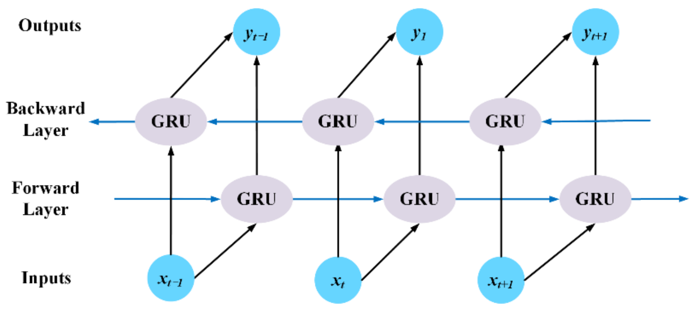
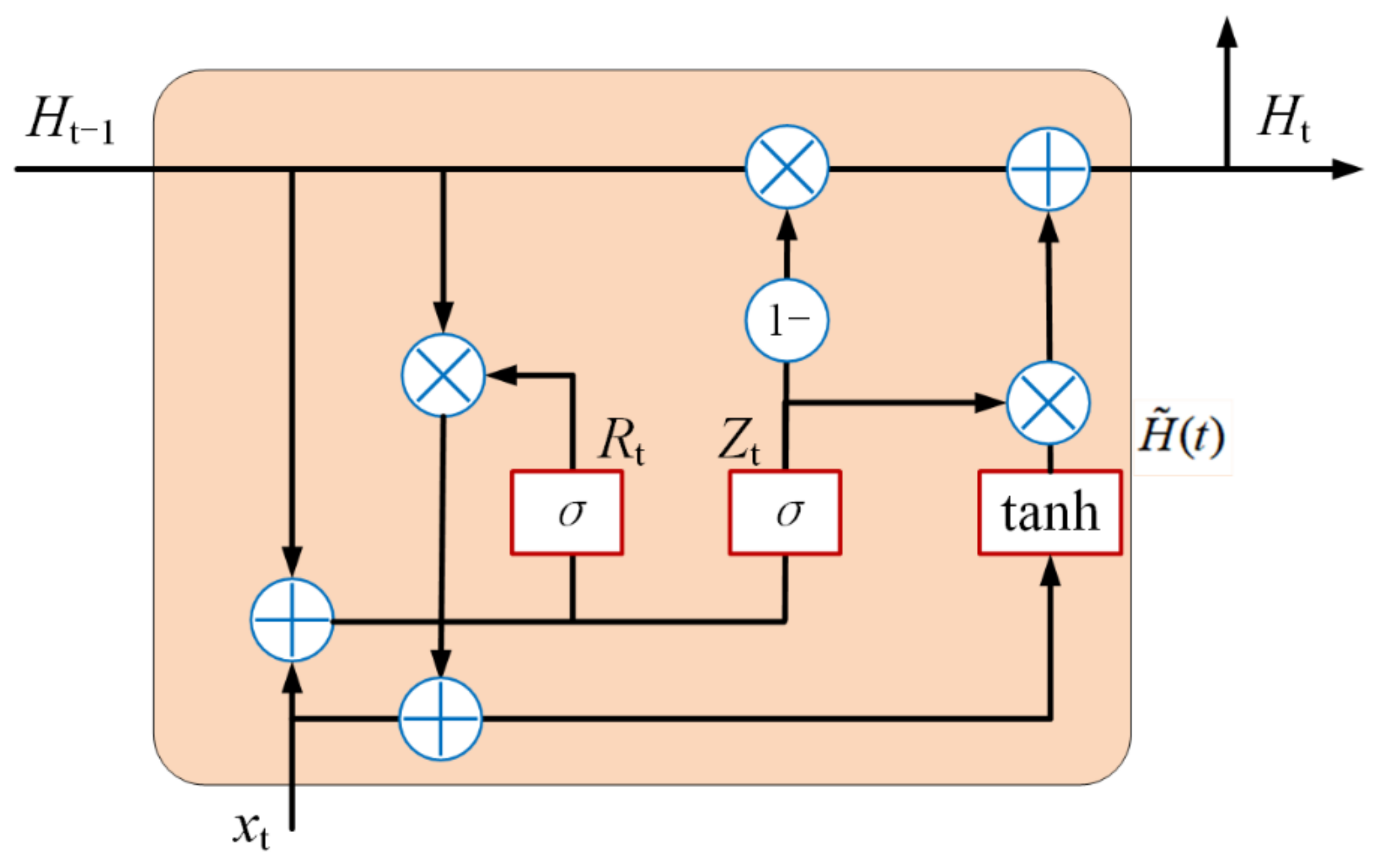
2.4. Bidirectional Gated Recurrent Unit

To analyze the feature vectors extracted by the SDAE and better learn the wave information of the axle temperatures from the historical multi-data, it is indispensable to apply an efficient time series forecasting model [57]. The GRU model, which is a kind of recurrent neural network (RNN), can be regarded as a simplified version of the LSTM model [58]. GRU integrates the units of the input gate and forget gate of LSTM so that it contains only the reset gate and update gate as the key components to form a GRU unit [59]. The update gate can control the extent of the current state information from the previous step. The size of the retained state information is proportional to the update gate value. Whereas the function of the reset gate is to determine the extent of the hidden layer information from the previous state, which should be deleted. More information will be deleted by a smaller reset gate [60]. The basic framework of GRU is shown in Figure 3. The GRU calculation formula is as follows [61]:

$$\mathrm{Z}(\mathrm{t})=\sigma \left({\mathrm{W}}_{\mathrm{Z}}·\left[\mathrm{H}\left(\mathrm{t}-1\right),{\mathrm{x}}_{\mathrm{t}}\right]\right)$$

(8)

$$\mathrm{R}(\mathrm{t})=\sigma \left({\mathrm{W}}_{\mathrm{R}}·\left[\mathrm{H}\left(\mathrm{t}-1\right),{\mathrm{x}}_{\mathrm{t}}\right]\right)$$

(9)

$$\tilde{\mathrm{H}}(\mathrm{t})=\tanh \left({\mathrm{W}}_{\tilde{\mathrm{H}}}·\left[\mathrm{R}\left(\mathrm{t}\right)\times \mathrm{H}\left(\mathrm{t}-1\right),{\mathrm{x}}_{\mathrm{t}}\right]\right)$$

(10)

$$\mathrm{H}(\mathrm{t})=\left(1-\mathrm{Z}\left(\mathrm{t}\right)\right)\times \mathrm{H}\left(\mathrm{t}-1\right)+\mathrm{Z}\left(\mathrm{t}\right)\times \mathrm{H}\left(\mathrm{t}\right)$$

(11)

where R(t) stands for the reset gate, Z(t) means the update gate, and σ represents the sigmoid activation function. $\tilde{\mathrm{H}}\left(\mathrm{t}\right)$ represents the candidate activation status information and H(t) represents the active status information.

The BIGRU is short for the bi-directional gated recurrent unit and it is architecturally composed of a forward-propagated GRU unit and a backward-propagated GRU unit [62]. The status information in a one-direction process will invariably transmit from the front to the back. However, the BIGRU connects two hidden layers with different directions for output, which may lead to more information to enhance the prediction process and improve the modeling performance [63]. The structure of the BIGRU is shown in Figure 4. The forward and backward layer values $\overrightarrow{\mathrm{H}}(\mathrm{t})$ $\overleftarrow{\mathrm{H}}(\mathrm{t})$ and final results $\mathrm{H}(\mathrm{t})$ are shown below.

$$\overrightarrow{\mathrm{H}}(\mathrm{t})=\mathrm{G}\mathrm{R}\mathrm{U}({\mathrm{x}}_{\mathrm{t}},\overrightarrow{\mathrm{H}}(\mathrm{t}-1))$$

(12)

$$\overleftarrow{\mathrm{H}}(\mathrm{t})=\mathrm{G}\mathrm{R}\mathrm{U}({\mathrm{x}}_{\mathrm{t}},\overleftarrow{\mathrm{H}}(\mathrm{t}-1))$$

(13)

$$\mathrm{H}(\mathrm{t})={\mathrm{w}}_{\mathrm{t}}\overrightarrow{\mathrm{H}}(\mathrm{t})+{\mathrm{v}}_{\mathrm{t}}\overleftarrow{\mathrm{H}}(\mathrm{t})+{\mathrm{b}}_{\mathrm{t}}$$

(14)

where w_t and v_t are weights relying on the forward or backward status of BIGRU, and b_t is the bias. The pseudocode of SDAE-BIGRU is listed in Algorithm 2.

Algorithm 2 The SDAE-BIGRU algorithms

Input: Selected features by Q-learning The weight set $\left[{\mathrm{W}}_{\mathrm{Z}},{\mathrm{W}}_{\mathrm{R}},{\mathrm{W}}_{\mathrm{H}}\right]$ in the BIGRU network The number of DAE layer k is l. The maximum number of SDAE epochs: Z The maximum number of BIGRU epochs: N Algorithm: Step1: Unsupervised layer training of SDAE 1: Initialize all parameters in the SDAE 2: for z = 1: Z do 3: for k = 1: l do 4: train the first layer of DAE and use the hidden layer as the input of the second DAE.    Repeat until the lth layer of DAE. 5: stack the trained n-layer DAE to obtain the SDAE with an output layer on the top 6: end for 7: end for The output will be transmitted as the optimal parameter into the BIGRU predictor Step2: Supervised layer training of BIGRU 1: Initialize all parameters in the BIGRU 2: for n = 1: N do 3: Calculate output in the single GRU $\mathrm{Z}(\mathrm{t})=\sigma \left({\mathrm{W}}_{\mathrm{Z}}·\left[\mathrm{H}\left(\mathrm{t}-1\right),{\mathrm{x}}_{\mathrm{t}}\right]\right), \mathrm{R}(\mathrm{t})=\sigma \left({\mathrm{W}}_{\mathrm{R}}·\left[\mathrm{H}\left(\mathrm{t}-1\right),{\mathrm{x}}_{\mathrm{t}}\right]\right)$ $\tilde{\mathrm{H}}(\mathrm{t})=\tanh \left({\mathrm{W}}_{\tilde{\mathrm{H}}}·\left[\mathrm{R}\left(\mathrm{t}\right)\times \mathrm{H}\left(\mathrm{t}-1\right),{\mathrm{x}}_{\mathrm{t}}\right]\right), \mathrm{H}(\mathrm{t})=\left(1-\mathrm{Z}\left(\mathrm{t}\right)\right)\times \mathrm{H}\left(\mathrm{t}-1\right)+\mathrm{Z}\left(\mathrm{t}\right)\times \mathrm{H}\left(\mathrm{t}\right)$ 4: Compute output in the Bi-directional structure $\overrightarrow{\mathrm{H}}(\mathrm{t})=\mathrm{G}\mathrm{R}\mathrm{U}({\mathrm{x}}_{\mathrm{t}},\overrightarrow{\mathrm{H}}(\mathrm{t}-1))\overleftarrow{\mathrm{H}}(\mathrm{t})=\mathrm{G}\mathrm{R}\mathrm{U}({\mathrm{x}}_{\mathrm{t}},\overleftarrow{\mathrm{H}}(\mathrm{t}-1))$ $\mathrm{H}(\mathrm{t})={\mathrm{w}}_{\mathrm{t}}\overrightarrow{\mathrm{H}}(\mathrm{t})+{\mathrm{v}}_{\mathrm{t}}\overleftarrow{\mathrm{H}}(\mathrm{t})+{\mathrm{b}}_{\mathrm{t}}$ (3) Iteration ends when the stopping criterion is satisfied. 5: end for Output: The forecasting results

3. Case Study

In this section, the proposed model will be evaluated in the case study to test its effectiveness and availability in the engineering application. The datasets, the evaluation indexes, and corresponding experiments are demonstrated in the following subsections.

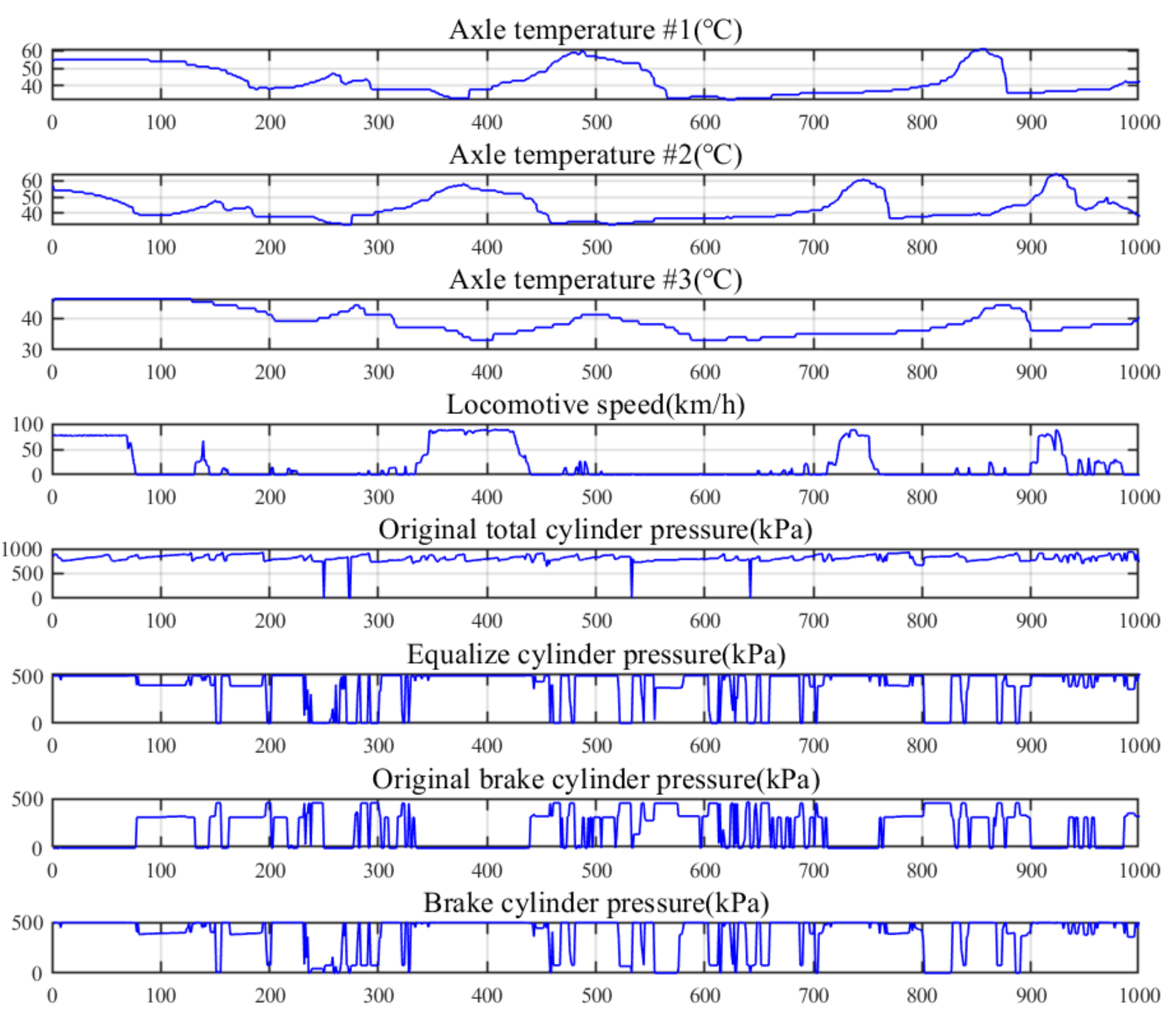
3.1. Locomotive Datasets

To fully verify the performance and application of the designed model, the datasets of 1000 samples were applied in the paper, which were collected during the locomotive operation period with a 1-min interval. The data has been preprocessed to remove outliers and smoothed for the sensor’s stepped data. The time series characteristics and the fluctuation information of the datasets are described in Figure 5 and Figure 6 shows the locomotive axle in the refurbishment test after the operation. The historical datasets include the axle temperatures from three axles in a bogie of the Harmony electric locomotive, the locomotive speeds, the original total cylinder pressures, the equalize cylinder pressures, the original brake cylinder pressures, and the brake cylinder pressures, in which the last five are used as auxiliary features in the feature selection process. In the experiments, the 1st–600th samples were regarded as the training set. The 601st–800th samples were selected as the validation set. The 801st–1000th samples were the test set. The experiments of this paper are conducted on Matlab2020, the Python 3.8.8 platform, and TensorFlow 2.3.0, which is run on a personal computer with Ci77700-2.81 GHz, 8 GB RAM, and Windows 10 64-bit operating system.

3.2. The Evaluation Indexes in the Study

The evaluation indexes will reflect the modeling forecasting performance. In the experiments, four indexes, namely the mean absolute error (MAE), the root mean square error (RMSE), the mean absolute percentage error (MAPE), and the standard deviation of error (SDE) were utilized to test the forecasting accuracy. What’s more, the promoting percentages of these indexes are also applied. These indexes are defined as below:

$$\left\{\begin{array}{l}\mathrm{MAE}=({\displaystyle \sum _{\mathrm{t}=1}^{\mathrm{n}}\left|\mathrm{r}(\mathrm{t})-\widehat{\mathrm{r}}(\mathrm{t})\right|})/\mathrm{n}\hfill \\ \mathrm{MAPE}=({\displaystyle \sum _{\mathrm{t}=1}^{\mathrm{n}}\left|(\mathrm{r}(\mathrm{t})-\widehat{\mathrm{r}}(\mathrm{t}))/\mathrm{r}(\mathrm{t})\right|})/\mathrm{n}\hfill \\ \mathrm{RMSE}=\sqrt{({\displaystyle \sum _{\mathrm{t}=1}^{\mathrm{n}}{\left[\mathrm{r}(\mathrm{t})-\widehat{\mathrm{r}}(\mathrm{t})\right]}^2)/\mathrm{n}}}\hfill \\ \mathrm{SDE}=\sqrt{({{\displaystyle \sum _{\mathrm{t}=1}^{\mathrm{n}}\left[\mathrm{r}(\mathrm{t})-\widehat{\mathrm{r}}(\mathrm{t})-{\displaystyle \sum _{\mathrm{t}=1}^{\mathrm{n}}(\mathrm{r}(\mathrm{t})-\widehat{\mathrm{r}}(\mathrm{t}))/\mathrm{n}}\right]}}^2)/\mathrm{n}}\hfill \end{array}\right.$$

(15)

$$\left\{\begin{array}{l}{\mathrm{P}}_{\mathrm{MAE}}=\left(\mathrm{MA}{\mathrm{E}}_1-\mathrm{MA}{\mathrm{E}}_2\right)/\mathrm{MA}{\mathrm{E}}_1\hfill \\ {\mathrm{P}}_{\mathrm{MAPE}}=\left(\mathrm{MAP}{\mathrm{E}}_1-\mathrm{MAP}{\mathrm{E}}_2\right)/\mathrm{MAP}{\mathrm{E}}_1\hfill \\ {\mathrm{P}}_{\mathrm{RMSE}}=\left(\mathrm{RMS}{\mathrm{E}}_1-\mathrm{RMS}{\mathrm{E}}_2\right)/\mathrm{RMS}{\mathrm{E}}_1\hfill \\ {\mathrm{P}}_{\mathrm{SD}\mathrm{E}}=\left(\mathrm{SD}{\mathrm{E}}_1-\mathrm{SD}{\mathrm{E}}_2\right)/\mathrm{SD}{\mathrm{E}}_1\hfill \end{array}\right.$$

(16)

where $\mathrm{r}(\mathrm{t})$ represents the raw data, $\widehat{\mathrm{r}}(\mathrm{t})$ is the forecasting result and n means the samples in raw datasets.

3.3. Comparing Analysis with Alternative Algorithms

In this section, the comparative experiment will be conducted by the main types of the proposed model to test each partial algorithm.

3.3.1. Comparative Experiment of Different Predictors

To verify the forecasting performance of the predictor BIGRU in time series modeling in-depth, the experiments will be conducted in comparison with some traditional shallow neural network predictors and classical deep learning predictors including LSTM, GRU, RNN, deep Boltzmann machine (DBM), evolutionary neural networks (ENN), extreme learning machine (ELM), multilayer perceptron (MLP), and radial basis function (RBF). Figure 7 and Figure 8 present statistical indexes of the prediction results. According to the experiment results, the following conclusions can be drawn:

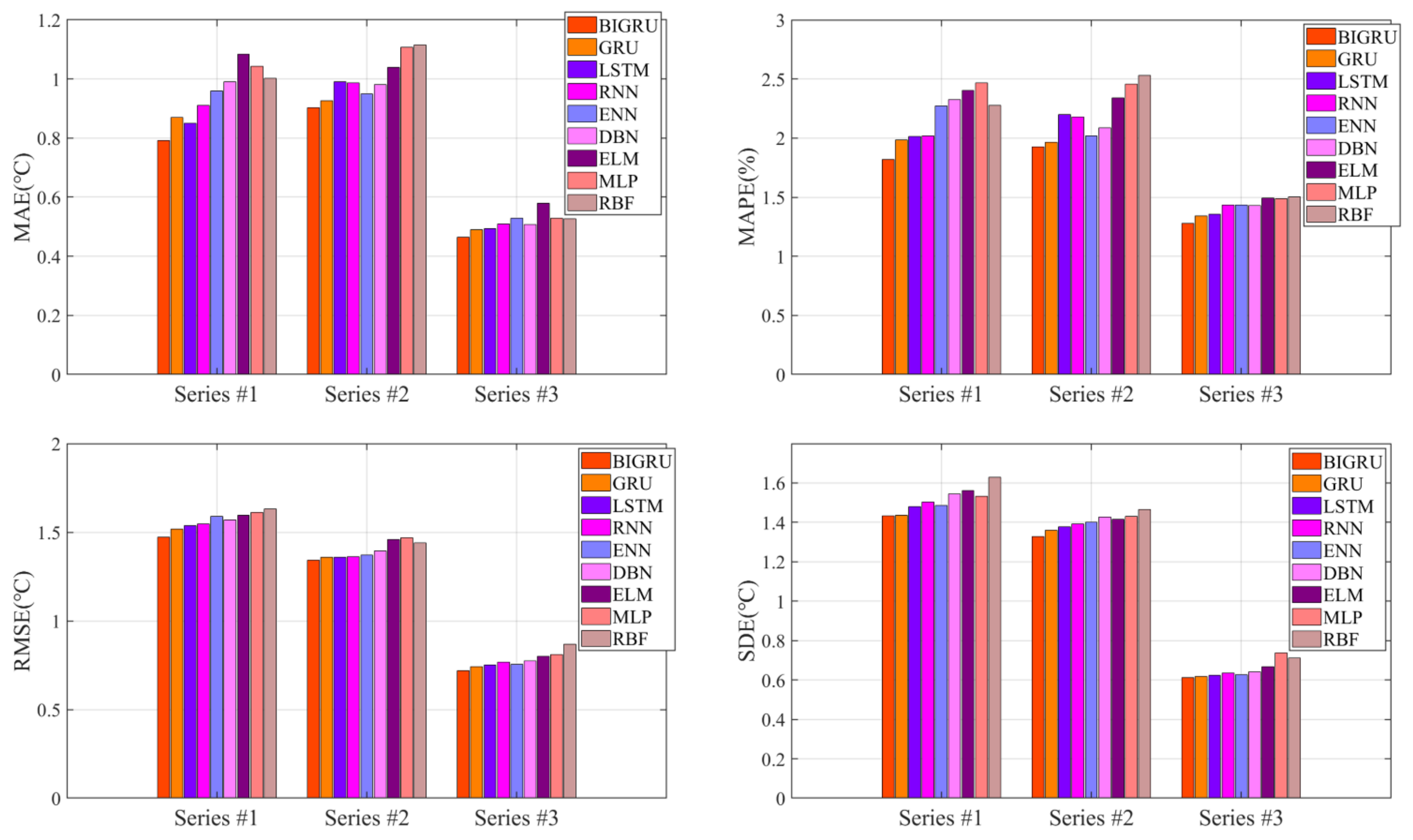
(1)

Compared to ELM, MLP, and RBF, other deep learning models with complex structures could obtain better axle temperature forecasting results. The forecasting accuracies of the traditional shallow neural network approaches are lower than deep learning models, which may be caused by the high fluctuation and irregular feature information of the original data. The deep learning algorithm, which could identify and analyze the series wave information by the multiple hidden layers, could effectively extract the deep information of the original data by an iterative process to obtain positive results.

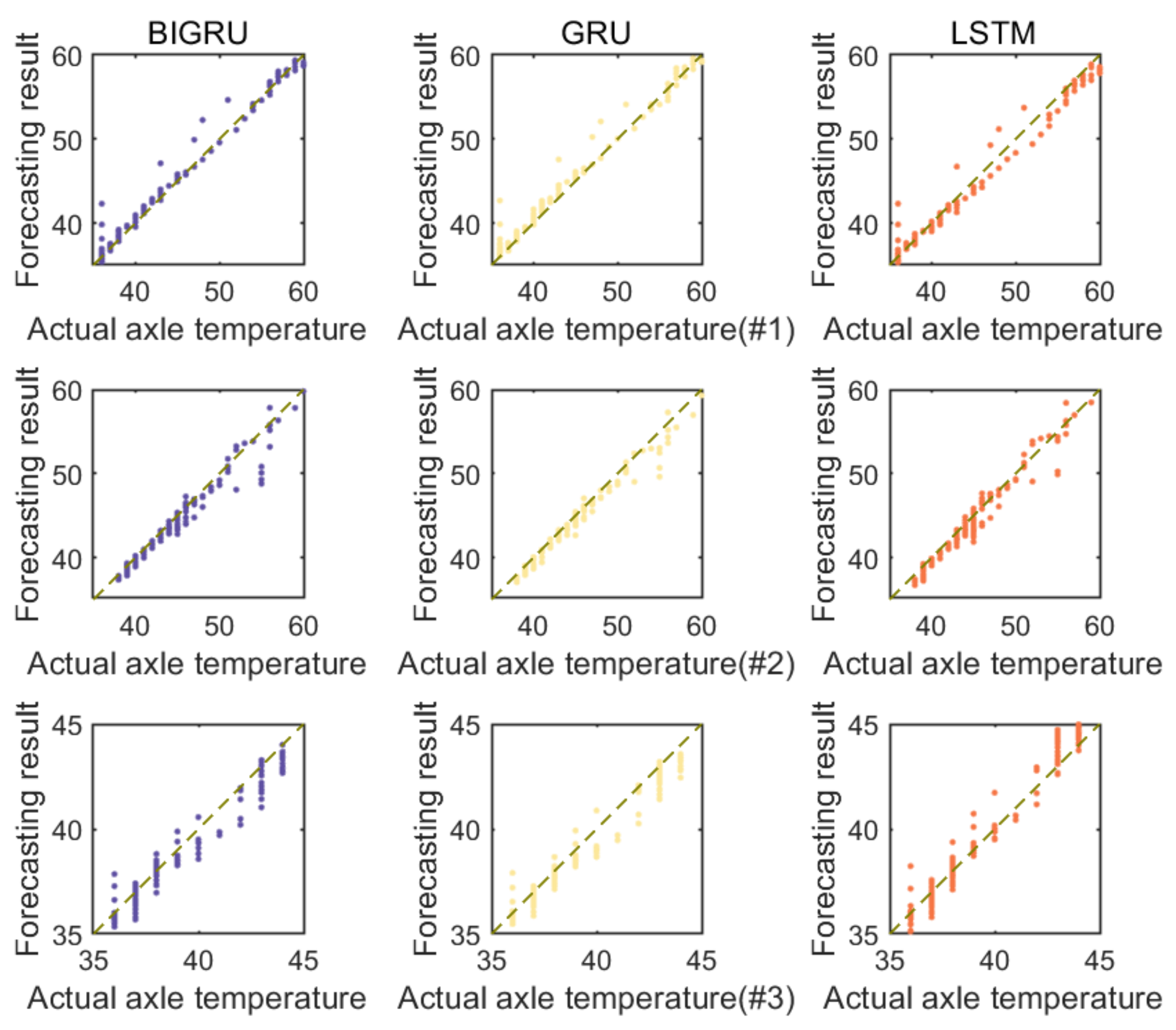
(2)

By the deep learning networks, the accuracies of GRU and LSTM in the results outperform others. The reason may be that the gated structure can efficiently ameliorate the process and select more information, which enables GRU and LSTM to analyze the characteristics of deep data fluctuation acquisition. Meanwhile, the prediction error of the BIGRU is lower than that of others and obtains the best forecasting results in all series. The feasible cause may be that the bidirectional operation structure could optimize the analytical capability for the core information to effectively improve the training ability and raise the calculation speed. However, for different axle temperature datasets of fluctuation characteristics, it can be observed that a single predictor is difficult to adapt to various cases. As a consequence, it is essential to utilize other algorithms to increase the applicability and recognition ability of the model.

Figure 7. Forecasting performance evaluation indexes: MAE, MAPE, RMSE, and SDE values of different predictors.

Figure 7. Forecasting performance evaluation indexes: MAE, MAPE, RMSE, and SDE values of different predictors.

Figure 8. Scatter plots of BIGRU, GRU, and LSTM.

Figure 8. Scatter plots of BIGRU, GRU, and LSTM.

3.3.2. Comparative Experiments and Analysis of Different Feature Extraction Methods

To fully prove the performance of the proposed feature extraction approach for the accuracy improvement of BIGRU in locomotive axle temperature forecasting, the experiments are conducted to compare the prediction results of SDAE-TCN and TCN. Moreover, the SDAE is also compared with SAE and PCA. Figure 9 presents statistical indexes of the prediction results and Table 1 lists the promoting percentages of the SDAE-BIGRU. According to the experiment results, the following conclusions can be drawn:

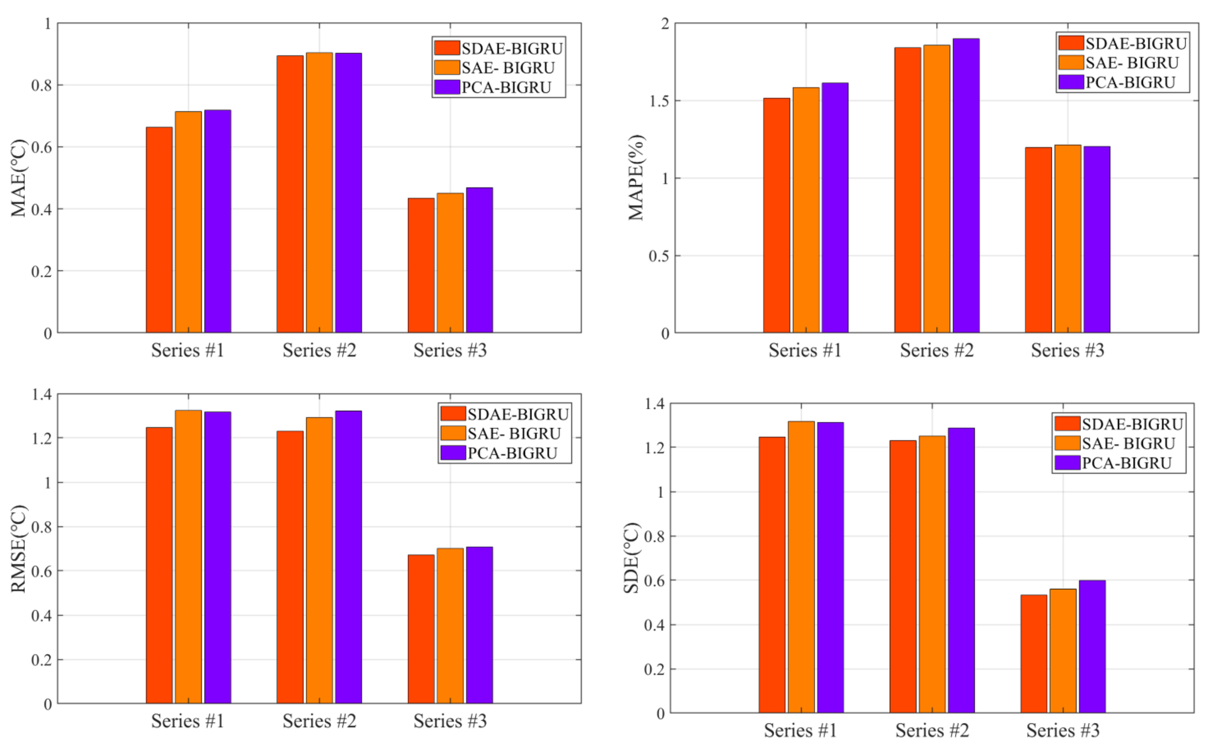
(1)

In contrast to single BIGRU predictors, the hybrid structure with a feature extraction algorithm can normally obtain better results with lower errors. The feature extraction algorithms effectively improve the prediction accuracy of the BIGRU, which extracts the input vector information and optimizes the fluctuation characteristics of the axle temperature datasets. The overall results showed that these feature extraction methods effectively raise the prediction accuracy in all cases. The probable reason may be that the feature extraction algorithms could deeply analyze the multi-data information and effectively reduce the modeling difficulty by raw data to promote the overall results.

(2)

By comparison with SAE and PCA methods, all results proved that the SDAE achieves the best results. SDAE can effectively decrease the data redundancy so that the recognition ability of the predictor can be further increased. Furthermore, the deep architecture of the SDAE is based on multi-layer DAE, which greatly increases the information extraction ability of the hybrid structure. Consequently, the feature selection approach based on SDAE is intensely effective for all datasets in axle temperature forecasting.

Figure 9. Forecasting performance evaluation indexes: MAE, MAPE, RMSE, and SDE values of different feature extraction methods.

Figure 9. Forecasting performance evaluation indexes: MAE, MAPE, RMSE, and SDE values of different feature extraction methods.

Table 1. The promoting percentages of the SDAE-BIGRU by the others.

Methods	Indexes	Series #1	Series #2	Series #3
SDAE-BIGRU vs. SAE- BIGRU	PMAE (%)	7.0247	0.8298	3.1263
	PMAPE (%)	4.4482	2.9477	1.4102
	PRMSE (%)	5.8370	4.7737	4.0274
	PSDE (%)	5.2867	1.6556	4.7917
SDAE-BIGRU vs. PCA- BIGRU	PMAE (%)	7.6462	0.9642	7.3119
	PMAPE (%)	6.1473	2.9477	0.4911
	PRMSE (%)	5.3941	6.8141	5.1383
	PSDE (%)	5.0270	4.5342	11.0127
SDAE-BIGRU vs. BIGRU	PMAE (%)	16.2541	1.1176	11.1565
	PMAPE (%)	16.7721	4.4492	6.3628
	PRMSE (%)	15.2911	8.3613	6.7314
	PSDE (%)	13.0474	7.3538	12.9618

Table 1. The promoting percentages of the SDAE-BIGRU by the others.

Methods	Indexes	Series #1	Series #2	Series #3
SDAE-BIGRU vs. SAE- BIGRU	PMAE (%)	7.0247	0.8298	3.1263
	PMAPE (%)	4.4482	2.9477	1.4102
	PRMSE (%)	5.8370	4.7737	4.0274
	PSDE (%)	5.2867	1.6556	4.7917
SDAE-BIGRU vs. PCA- BIGRU	PMAE (%)	7.6462	0.9642	7.3119
	PMAPE (%)	6.1473	2.9477	0.4911
	PRMSE (%)	5.3941	6.8141	5.1383
	PSDE (%)	5.0270	4.5342	11.0127
SDAE-BIGRU vs. BIGRU	PMAE (%)	16.2541	1.1176	11.1565
	PMAPE (%)	16.7721	4.4492	6.3628
	PRMSE (%)	15.2911	8.3613	6.7314
	PSDE (%)	13.0474	7.3538	12.9618

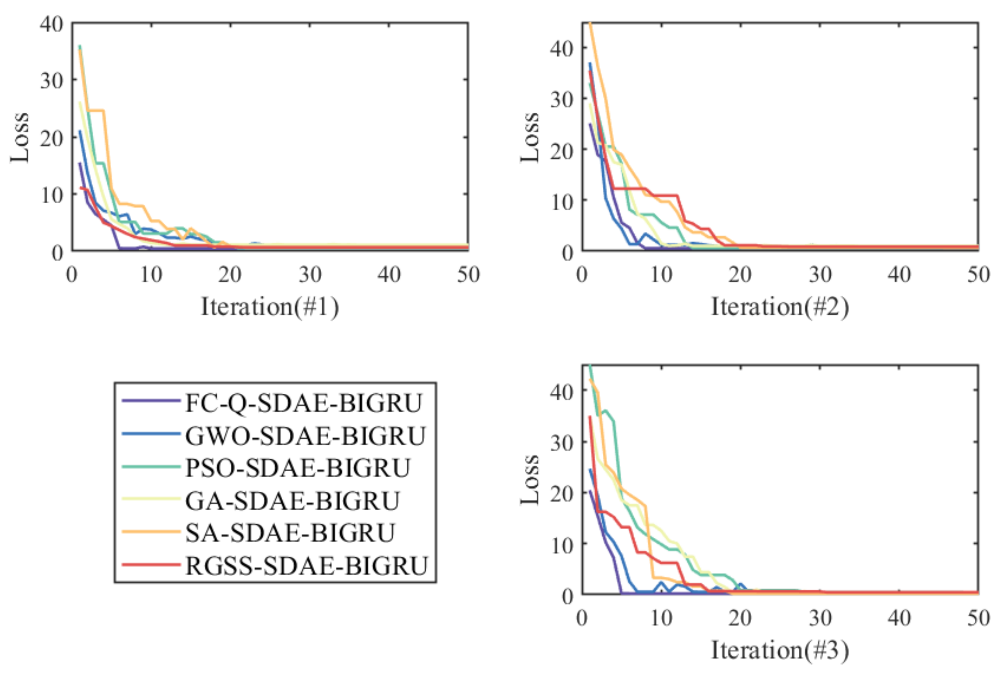
3.3.3. Comparative Experiments of Different Feature Selection Methods

To evaluate and test the performance of the Q-learning-based feature selection approach, the FC-Q-SDAE-BIGRU model is compared with the SDAE-BIGRU to prove the effectiveness of the feature selection method in decreasing modeling input redundancy and forecasting errors. Furthermore, to prove the favorable application of the reinforcement learning algorithm in feature selection, the Q-learning algorithm is also tested with traditional meta-heuristic algorithms like the genetic algorithm (GA), gray wolf optimization (GWO), particle swarm optimization (PSO), simulated annealing (SA), and random generation plus sequential selection (RGSS), respectively. The results are presented in Figure 10 and Table 2. Table 3 displays the feature selection results obtained by the Q-learning algorithm, which can fully list the influence of various feature information on the prediction accuracy of axle temperature in detail. Figure 11 shows the values of Loss during the iterations of Q-learning, GWO, PSO, GA, SA, and RGSS. Based on the experiment results, it can be concluded that:

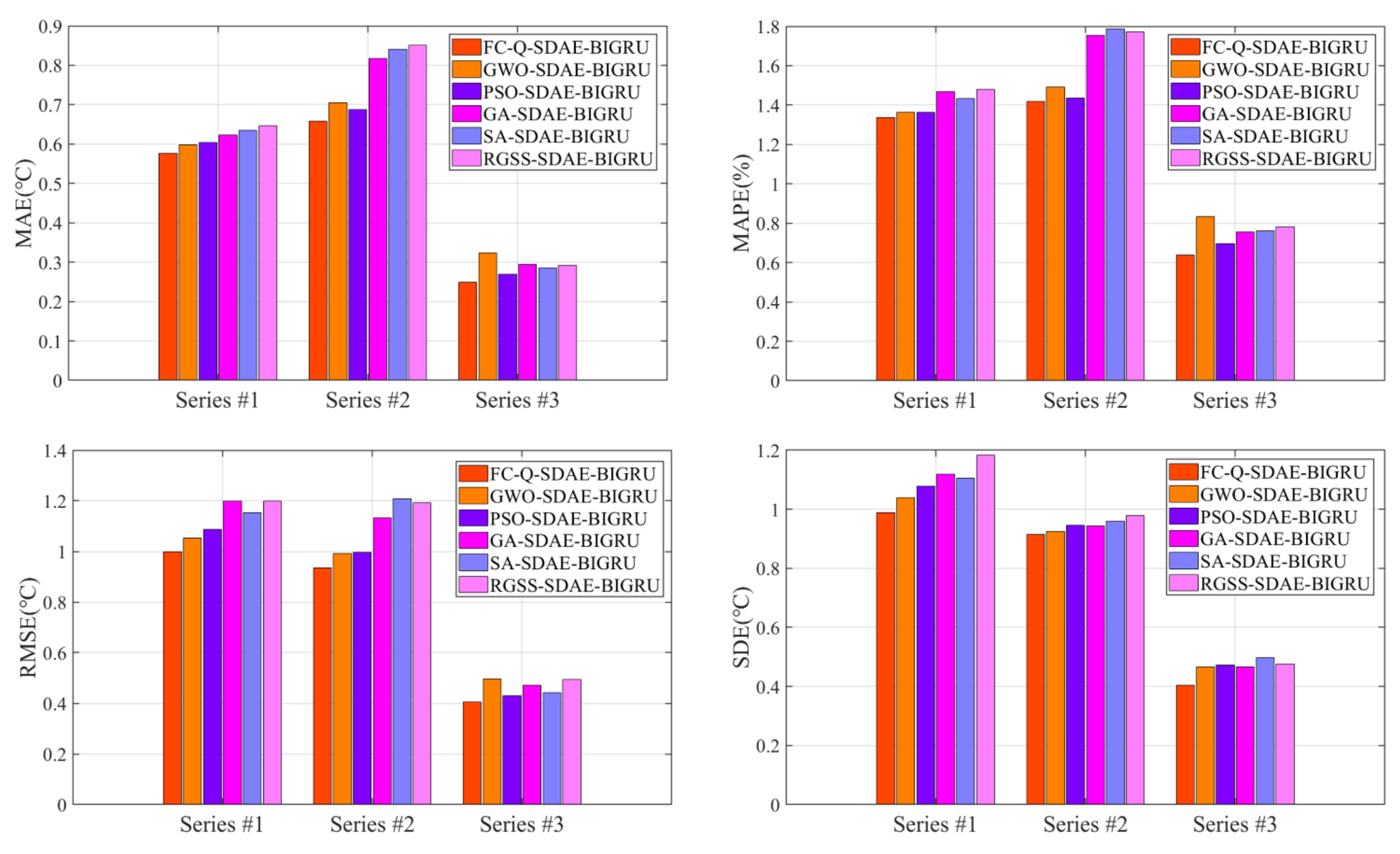
(1)

The experimental results fully prove the ability of the feature selection algorithm to raise the prediction accuracy of SDAE-BIGRU in all cases. The possible reason is that the two-stage feature selection algorithms applied in this paper can unearth the deep correlation between axel temperature and other locomotive feature historical data, and selects the suitable features of the best quality, which could effectively avoid overfitting and obtain the best input for BIGRU.

(2)

By comparison with the traditional heuristic algorithms, the forecasting accuracy of the models with the reinforcement learning algorithm as feature selection is better than other methods in all datasets. Different from the population iteration process of the heuristic algorithms, the reinforcement learning algorithm improves the intelligence of the hybrid model by constantly training agents. By analyzing the relevance between input and output results, Q-learning could raise the decision-making ability and select the optimal features of axle temperature modeling.

(3)

The locomotive speeds and the cylinder pressures also have a great influence on the prediction results of FC-Q-SDAE-BIGRU. As the key component of the transmission system, the cylinder pressures can reflect the control status of the bogie. The speed is also a direct signal in the driven status of locomotives. In addition, the historical information on axle temperature could efficiently reflect the changing trend with the assistance of multiple auxiliary datasets. Therefore, these variables play a crucial role in establishing the prediction model. An accurate forecasting framework can conduct a precise estimation of future data changes so that the drivers and the train control centers can make accurate adjustments to stabilize the vehicles and avoid accidents.

Figure 10. Forecasting performance evaluation indexes: MAE, MAPE, RMSE, and SDE values of different feature selection methods.

Figure 10. Forecasting performance evaluation indexes: MAE, MAPE, RMSE, and SDE values of different feature selection methods.

Figure 11. Values of Loss during the iterations of Q-learning, GWO, PSO, GA, SA, and RGSS in series #1, #2, and #3.

Figure 11. Values of Loss during the iterations of Q-learning, GWO, PSO, GA, SA, and RGSS in series #1, #2, and #3.

Table 2. The promoting percentages of the FC-Q-SDAE-BIGRU by the others.

Methods	Indexes	Series #1	Series #2	Series #3
FC-Q-SDAE-BIGRU vs. GWO-SDAE-BIGRU	PMAE (%)	3.8403	6.5267	22.8677
	PMAPE (%)	2.0378	5.0379	23.3769
	PRMSE (%)	5.2122	5.7531	18.5088
	PSDE (%)	4.9913	0.9963	13.2719
FC-Q-SDAE-BIGRU vs. PSO-SDAE-BIGRU	PMAE (%)	4.7154	4.2024	7.5213
	PMAPE (%)	2.0377	1.3020	8.3931
	PRMSE (%)	8.1762	6.1503	5.7634
	PSDE (%)	8.4175	3.2797	14.2463
FC-Q-SDAE-BIGRU vs. GA-SDAE-BIGRU	PMAE (%)	7.5454	19.4326	15.2749
	PMAPE (%)	8.9646	19.2124	15.3632
	PRMSE (%)	16.7306	17.4696	13.9796
	PSDE (%)	11.7552	3.1363	13.3462
FC-Q-SDAE-BIGRU vs. SA-SDAE-BIGRU	PMAE (%)	9.1784	21.6088	12.4518
	PMAPE (%)	6.8321	20.6416	16.2403
	PRMSE (%)	13.4685	22.4770	8.3616
	PSDE (%)	10.6700	4.7808	18.7424
FC-Q-SDAE-BIGRU vs. RGSS-SDAE-BIGRU	PMAE (%)	10.8928	22.5579	14.2563
	PMAPE (%)	9.6355	20.0147	18.2668
	PRMSE (%)	16.6820	21.5992	17.7818
	PSDE (%)	16.5202	6.6571	15.0032

Table 2. The promoting percentages of the FC-Q-SDAE-BIGRU by the others.

Methods	Indexes	Series #1	Series #2	Series #3
FC-Q-SDAE-BIGRU vs. GWO-SDAE-BIGRU	PMAE (%)	3.8403	6.5267	22.8677
	PMAPE (%)	2.0378	5.0379	23.3769
	PRMSE (%)	5.2122	5.7531	18.5088
	PSDE (%)	4.9913	0.9963	13.2719
FC-Q-SDAE-BIGRU vs. PSO-SDAE-BIGRU	PMAE (%)	4.7154	4.2024	7.5213
	PMAPE (%)	2.0377	1.3020	8.3931
	PRMSE (%)	8.1762	6.1503	5.7634
	PSDE (%)	8.4175	3.2797	14.2463
FC-Q-SDAE-BIGRU vs. GA-SDAE-BIGRU	PMAE (%)	7.5454	19.4326	15.2749
	PMAPE (%)	8.9646	19.2124	15.3632
	PRMSE (%)	16.7306	17.4696	13.9796
	PSDE (%)	11.7552	3.1363	13.3462
FC-Q-SDAE-BIGRU vs. SA-SDAE-BIGRU	PMAE (%)	9.1784	21.6088	12.4518
	PMAPE (%)	6.8321	20.6416	16.2403
	PRMSE (%)	13.4685	22.4770	8.3616
	PSDE (%)	10.6700	4.7808	18.7424
FC-Q-SDAE-BIGRU vs. RGSS-SDAE-BIGRU	PMAE (%)	10.8928	22.5579	14.2563
	PMAPE (%)	9.6355	20.0147	18.2668
	PRMSE (%)	16.6820	21.5992	17.7818
	PSDE (%)	16.5202	6.6571	15.0032

Table 3. Feature selection results of reinforcement learning method for the axle temperatures series.

Series	Time	Locomotive Speeds	Original Total Cylinder Pressures	Equalize Cylinder Pressures	Original Brake Cylinder Pressures	Brake Cylinder Pressures	Axle Temperature
#1	T-5	0	0	0	0	0	0
	T-4	1	0	0	1	0	1
	T-3	1	1	1	1	0	0
	T-2	1	0	0	1	1	0
	T-1	0	0	0	0	1	0
#2	T-5	0	0	1	1	0	1
	T-4	1	1	0	0	0	1
	T-3	0	0	1	1	0	1
	T-2	0	0	0	0	1	0
	T-1	1	1	0	1	1	0
#3	T-5	0	1	0	0	1	1
	T-4	1	1	1	0	1	0
	T-3	1	0	0	1	1	1
	T-2	1	1	0	1	1	0
	T-1	0	1	1	1	1	1

Table 3. Feature selection results of reinforcement learning method for the axle temperatures series.

Series	Time	Locomotive Speeds	Original Total Cylinder Pressures	Equalize Cylinder Pressures	Original Brake Cylinder Pressures	Brake Cylinder Pressures	Axle Temperature
#1	T-5	0	0	0	0	0	0
	T-4	1	0	0	1	0	1
	T-3	1	1	1	1	0	0
	T-2	1	0	0	1	1	0
	T-1	0	0	0	0	1	0
#2	T-5	0	0	1	1	0	1
	T-4	1	1	0	0	0	1
	T-3	0	0	1	1	0	1
	T-2	0	0	0	0	1	0
	T-1	1	1	0	1	1	0
#3	T-5	0	1	0	0	1	1
	T-4	1	1	1	0	1	0
	T-3	1	0	0	1	1	1
	T-2	1	1	0	1	1	0
	T-1	0	1	1	1	1	1

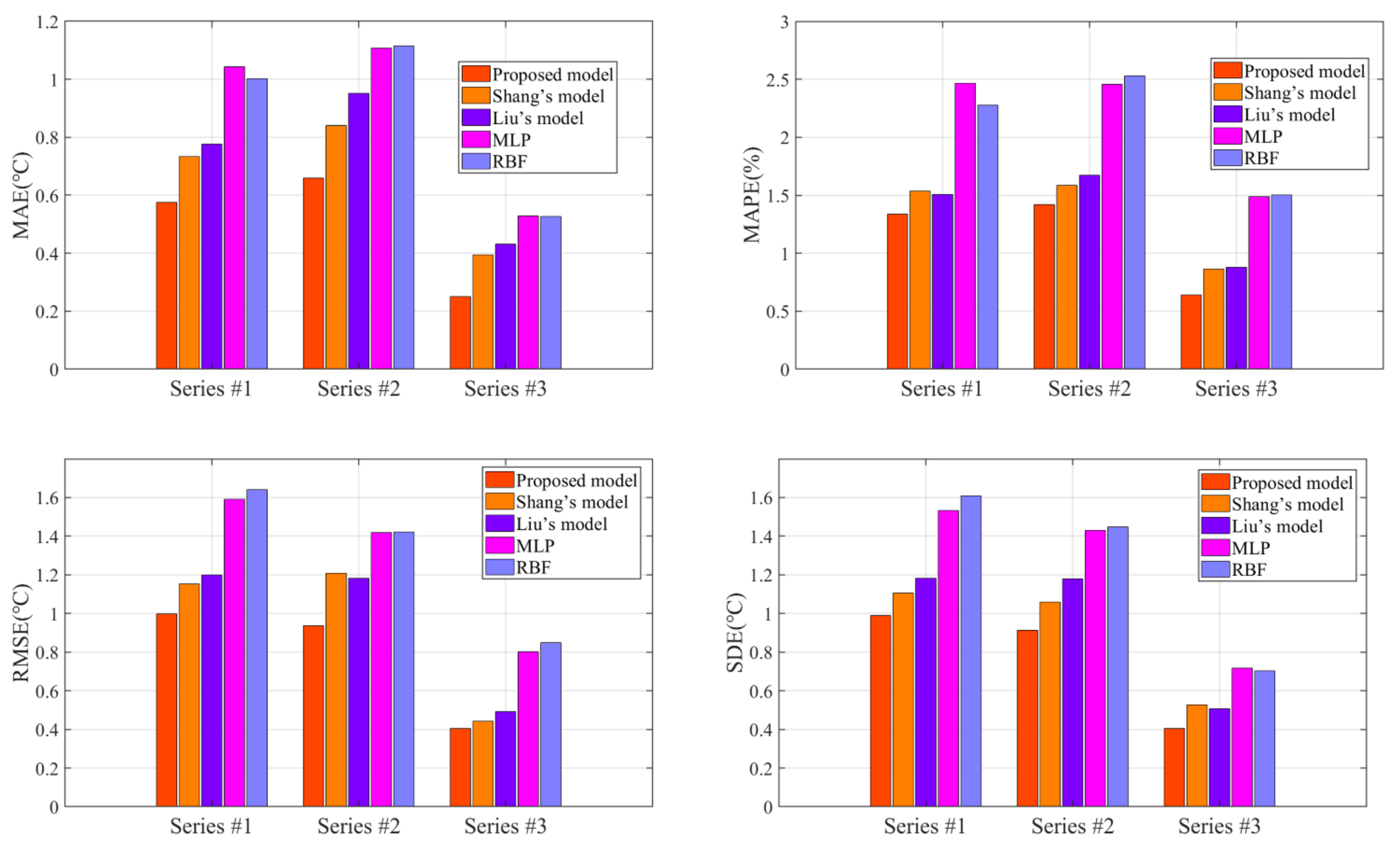
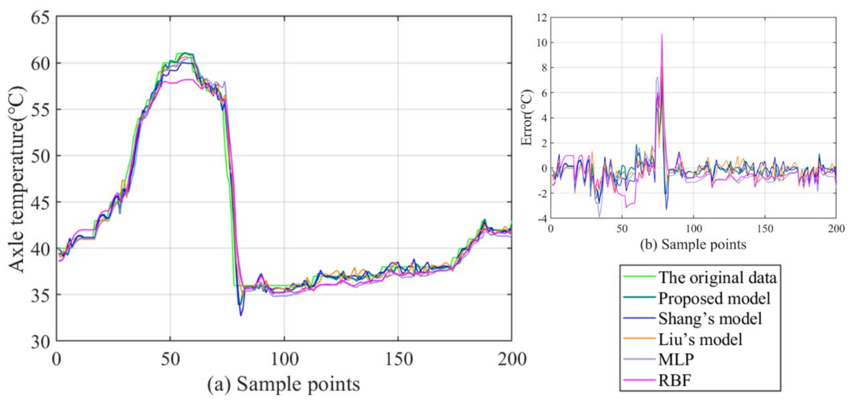
3.4. Comparative Experiments with Benchmark Models

To verify the availability and advancement of the proposed FC-Q-SDAE-BIGRU model, comparative experiments are conducted in the analysis with two existing state-of-the-art models in time series forecasting, namely Shang’s model [12], and Liu’s model [13] and two kinds of classic models, which are MLP and RBF. These state-of-the-art models have obtained positive results. Figure 12 presents the evaluation index values of all the benchmark models. Figure 13, Figure 14 and Figure 15 display the results of the proposed model and other existing models. Based on the comparative results, it could be summarized as follows:

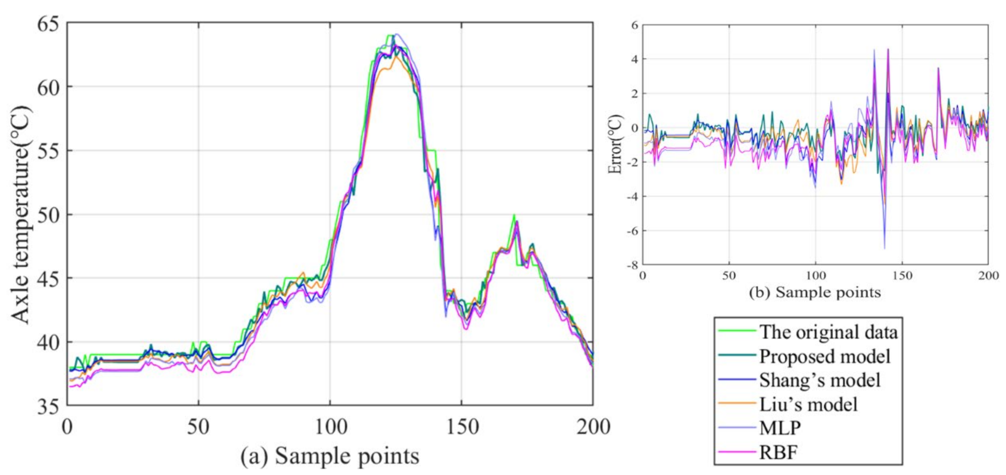
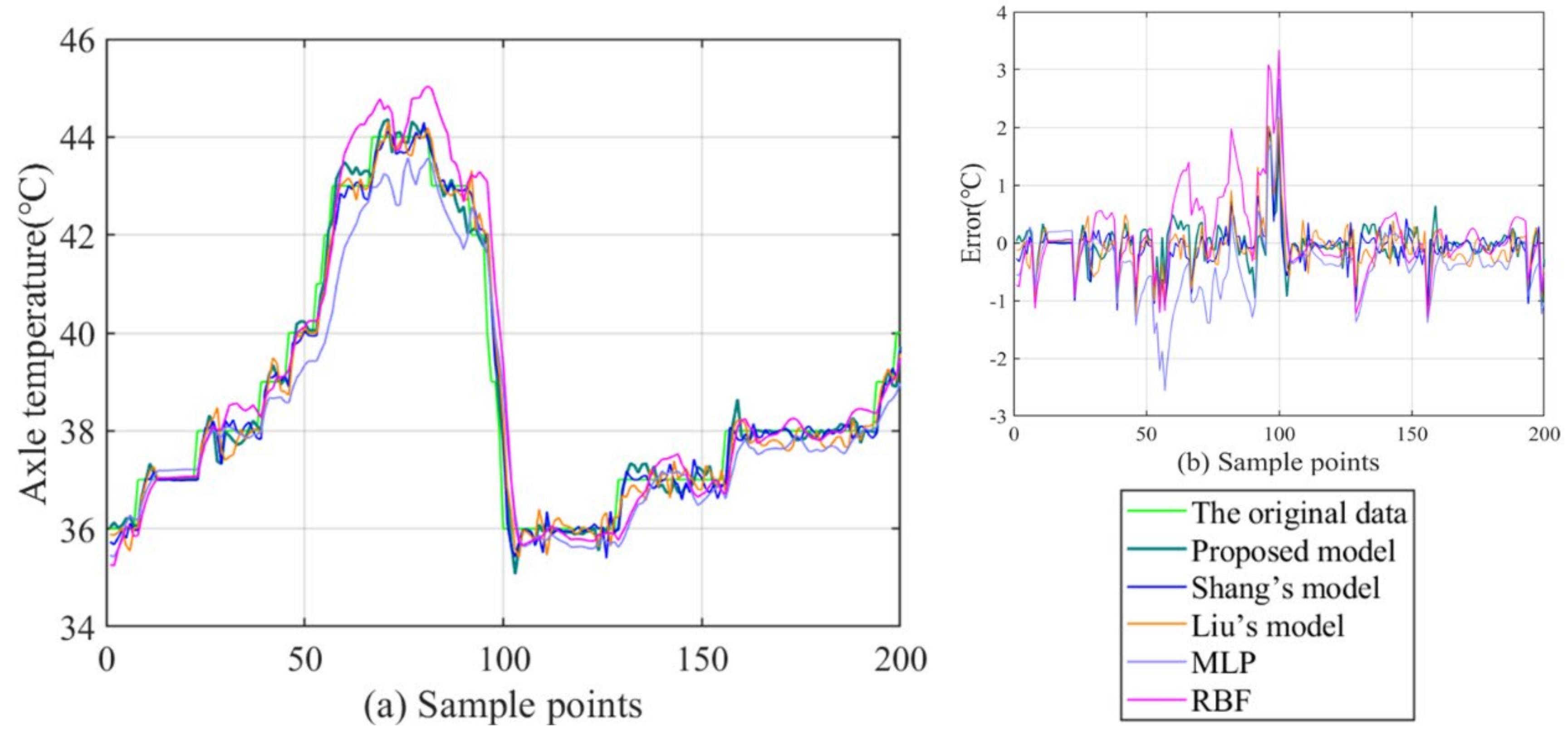
(1)

By comparison with the MLP and RBF, other hybrid ensemble models can achieve more satisfactory axle temperature modeling results. The single predictor can explore the simple nonlinear relation of the raw data, but it is arduous to follow the deep fluctuation information and the multi-data effect. On the contrary, the hybrid models can effectively integrate the advantages of each component and accomplish a valid modeling structure based on the multi-data.

(2)

In the above models, the proposed model acquires the best results with lower errors in all cases. This fully demonstrates that the FC-Q-SDAE-BIGRU framework is of favorable scientific modeling value, and combines the advantages of feature analysis and deep learning. A multi-data-driven axle temperature forecasting framework was utilized to construct more detailed mapping relationships than univariate models, and ensure that more influencing factors will be taken into account. The reinforcement learning-based two-step feature selection and SDAE-based feature extraction approaches were applied to improve the modeling input, analyze the advantageous information, and decrease the redundancy from raw data features. Finally, the application of the BIGRU model has also further improved the forecasting accuracy of classical deep learning methods.

Figure 12. Forecasting performance evaluation indexes: MAE, MAPE, RMSE, and SDE values of the proposed model and existing models.

Figure 12. Forecasting performance evaluation indexes: MAE, MAPE, RMSE, and SDE values of the proposed model and existing models.

Figure 13. Prediction results and errors of series #1: (a) prediction results; (b) error distribution.

Figure 13. Prediction results and errors of series #1: (a) prediction results; (b) error distribution.

Figure 14. Prediction results and errors of series #2: (a) prediction results; (b) error distribution.

Figure 14. Prediction results and errors of series #2: (a) prediction results; (b) error distribution.

Figure 15. Prediction results and errors of series #3: (a) prediction results; (b) error distribution.

Figure 15. Prediction results and errors of series #3: (a) prediction results; (b) error distribution.

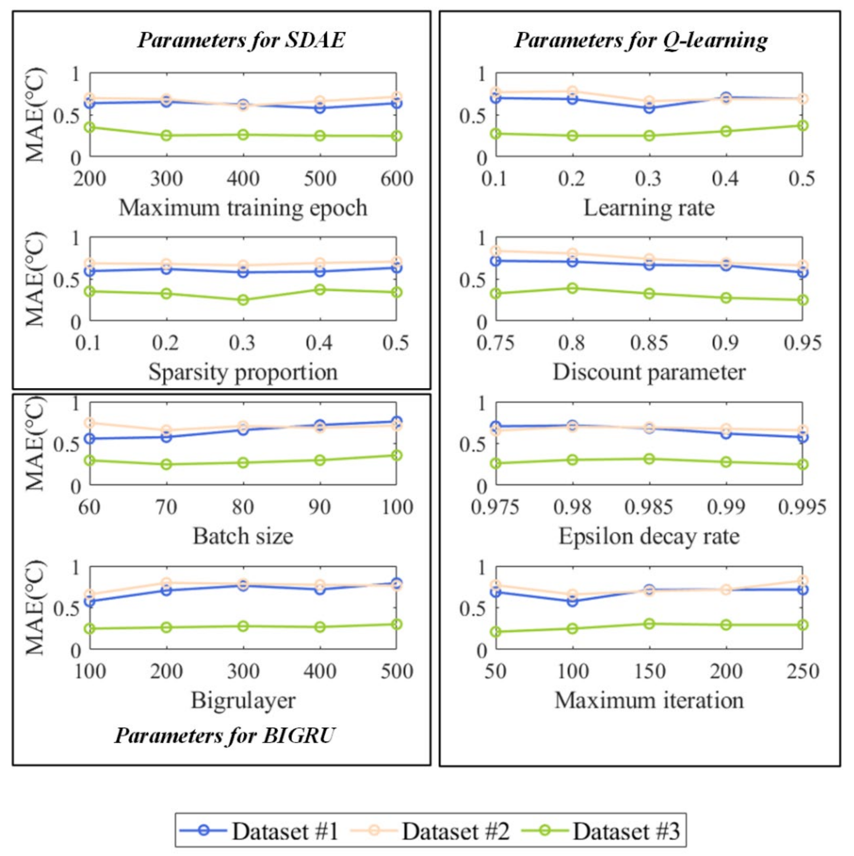
3.5. Sensitive Analysis of the Parameters and the Computational Time

The parameters of the algorithms play an important role in the modeling experiments. For example, the maximum number of training epochs control the rounds or iterations of the algorithm, which could directly limit the operation time. The sparsity proportion is the parameter of the sparsity regularizer, which controls the sparsity of the hidden layer output [64]. The batch size affects the optimization degree, the speed of the model, and the conditions of the GPU. The learning rate determines whether and when the objective function converges to a local minimum [65]. Briefly, the parameters could affect the direction, speed, and scope of modeling optimization, data selection, and feature extraction. The performance of the model is directly related to the selection and correlation of these parameters and the application of different datasets. To achieve better prediction accuracy, it is necessary to compare and adjust the model parameters.

In this section, the sensitivity of the parameters in the proposed framework is analyzed. The parameters are tested by five different values in three axle temperature datasets. The sensitivity analysis results of the important parameters in the proposed model are presented in Figure 16. The MAEs are utilized to represent the model forecasting accuracy. It can be found from the graphic results that the proposed model is generally stable and robust to the parameters with a few fluctuations in different datasets. For example, when the discount parameter is 0.95, the MAEs have the smallest values in all datasets, which stands for the best forecasting accuracy. In the maximum iterations of Q-learning, the changing of the parameter value has little influence on the results. To save computational time, it is rational to set the maximum iterations as 100.

Based on

Table 4. The average computational time of different models in the axle temperature dataset.

Algorithms	Computational Time
BIGRU	42.61 s
GRU	25.45 s
LSTM	28.85 s
ELM	12.41 s
MLP	15.93 s
SAE- BIGRU	53.42 s
GA-SDAE-BIGRU	107.67 s
GWO-SDAE-BIGRU	99.43 s
PSO-SDAE-BIGRU	93.26 s
FC-Q-SDAE-BIGRU	124.08 s

, it can be determined that the average calculation time of the hybrid model is more than that of the single models in the datasets of this paper. The time costs of deep learning models are also higher than the traditional shallow neural networks, which may be caused by the complex network structure and more hidden layers. With the application of various optimization methods, feature extraction, feature selection, etc., the structure of the hybrid model tends to diversify, which could effectively extract the deep information of the original data by an iterative process to obtain positive results. Aside from the improvement in model forecasting accuracy, these complex structures also intensify the expansion of computational cost and time.

The calculation cost of the proposed model is also given in

Table 5. The computational time of the proposed model.

Algorithms	Computational Time
FC-Q	61.05 s
SDAE	20.42 s
BIGRU	42.61 s
Total	124.08 s

. The parts of the models contribute to the best accuracy of other benchmark models with higher time costs. Considering the dataset of 1000 samples with the output of 200 samples from the normal operation, the model effectively predicts the changing trend of axial temperature under a certain time consumption. For predictions over a longer time horizon, it may be necessary to increase the time interval with the updated sensor data process to effectively evaluate the accuracy and availability of the model.

4. Conclusions and Future Work

The axle temperature forecasting could render a technical analysis for the status detection of locomotives. In pursuit of forecasting accuracy, a novel multi-data-driven model based on reinforcement learning and deep learning is proposed in the research, which consists of the reinforcement learning feature selection, the SDAE feature extraction, and the BIGRU neural network. The study can be elaborated from the following perspectives:

(1)

This paper analyzes the influence of multi-factor inputs on axle temperature forecasting modeling. The FC-Q-SDAE-BIGRU framework could deeply recognize the wave features of the raw data and analyze the influence of input features on forecasting modeling of the changing trend. The experimental results show that the auxiliary inputs are beneficial to accomplishing accurate forecasting.

(2)

From the comparative experiments, it could be found that the existing single predictors are not able to extract deep nonlinear characteristics to acquire satisfying results. Different from the traditional single predictor time series forecasting framework, the study designed a multi-data-driven hybrid forecasting model.

(3)

A new two-stage feature selection structure could be utilized to preprocess an original input. The FC method could further explore the potential features of the raw data and the reinforcement learning algorithm (Q-learning) comprehensively, considering the influence of other features from different angles on axle temperature, which helps to select the optimal features. SDAE method effectively extracts the deep cognition of the features and eliminates data redundancy, which significantly improves the modeling capability. Based on the principle of GRU and RNN, the bidirectional operation framework of GRU possess excellent time series modeling and forecasting ability that BIRGU revealed positive analytical capability and forecasting accuracy by comparison to other deep learning models and traditional neural network predictors.

(4)

The multi-data forecasting model combining the reinforcement learning and deep learning presented in the paper integrated the advancement of each component. In general, the proposed framework proved to be better than the benchmark models in all cases, which described excellent applicability to axle temperature forecasting.

The axle temperature model presented in the study renders technical support for the intelligent control of locomotives and early warning. Based on the historical data, the forecasting process could output judgments about the future operation trend of railway vehicles, which also contributes to predictive maintenance to decrease operation costs. The modeling framework can be also applied for the analysis of other time series data of railway vehicles and other engineering fields. For future research, the framework could be optimized and expanded from the following aspects to enhance the practical value:

(1)

Besides the axle temperature data, the influence of other factors such as power consumption, locomotive ambient temperature, and maintenance engineering plan on the abnormal trends of temperature data is also worth further studying.

(2)

During the life cycle, a huge amount of data will continue to accumulate with the operation of the locomotive so the forecasting model must also be constantly updated. Moreover, the intelligent big data platform could accomplish model parallel computing and analysis ability. In the future, the proposed model can be embedded into an intelligent big data platform such as Spark to further improve the comprehensive performance of the model and to establish an intelligent railway vehicle system. The systematic integration of data and models deserves further study.

References

- Ghaviha, N.; Campillo, J.; Bohlin, M.; Dahlquist, E. Review of application of energy storage devices in railway transportation. Energy Procedia 2017, 105, 4561–4568. [Google Scholar] [CrossRef]
- Wu, S.C.; Liu, Y.X.; Li, C.H.; Kang, G.; Liang, S.L. On the fatigue performance and residual life of intercity railway axles with inside axle boxes. Eng. Fract. Mech. 2018, 197, 176–191. [Google Scholar] [CrossRef]
- Yan, G.; Yu, C.; Bai, Y. A New Hybrid Ensemble Deep Learning Model for Train Axle Temperature Short Term Forecasting. Machines 2021, 9, 312. [Google Scholar] [CrossRef]
- Milic, S.D.; Sreckovic, M.Z. A Stationary System of Noncontact Temperature Measurement and Hotbox Detecting. IEEE Trans. Veh. Technol. 2008, 57, 2684–2694. [Google Scholar] [CrossRef]
- Li, C.; Luo, S.; Cole, C.; Spiryagin, M. An overview: Modern techniques for railway vehicle on-board health monitoring systems. Veh. Syst. Dyn. 2017, 55, 1045–1070. [Google Scholar] [CrossRef]
- Vale, C.; Bonifácio, C.; Seabra, J.; Calçada, R.; Mazzino, N.; Elisa, M.; Terribile, S.; Anguita, D.; Fumeo, E.; Saborido, C. Novel efficient technologies in Europe for axle bearing condition monitoring—The MAXBE project. Transp. Res. Procedia 2016, 14, 635–644. [Google Scholar] [CrossRef]
- Liu, Q. High-speed Train Axle Temperature Monitoring System Based on Switched Ethernet. Procedia Comput. Sci. 2017, 107, 70–74. [Google Scholar] [CrossRef]
- Bing, C.; Shen, H.; Jie, C.; Li, L. Design of CRH axle temperature alarm based on digital potentiometer. In Proceedings of the Chinese Control Conference, Chengdu, China, 27–29 July 2016. [Google Scholar]
- Yan, G.; Yu, C.; Bai, Y. Wind Turbine Bearing Temperature Forecasting Using a New Data-Driven Ensemble Approach. Machines 2021, 9, 248. [Google Scholar] [CrossRef]
- Mi, X.; Zhao, S. Wind speed prediction based on singular spectrum analysis and neural network structural learning. Energy Convers. Manag. 2020, 216, 112956. [Google Scholar] [CrossRef]
- Wang, H.; Li, G.; Wang, G.; Peng, J.; Jiang, H.; Liu, Y. Deep learning based ensemble approach for probabilistic wind power forecasting. Appl. Energy 2017, 188, 56–70. [Google Scholar] [CrossRef]
- Shang, P.; Liu, X.; Yu, C.; Yan, G.; Xiang, Q.; Mi, X. A new ensemble deep graph reinforcement learning network for spatio-temporal traffic volume forecasting in a freeway network. Digit. Signal Processing 2022, 123, 103419. [Google Scholar] [CrossRef]
- Liu, X.; Qin, M.; He, Y.; Mi, X.; Yu, C. A new multi-data-driven spatiotemporal PM2. 5 forecasting model based on an ensemble graph reinforcement learning convolutional network. Atmos. Pollut. Res. 2021, 12, 101197. [Google Scholar] [CrossRef]
- Yan, G.; Chen, J.; Bai, Y.; Yu, C.; Yu, C. A Survey on Fault Diagnosis Approaches for Rolling Bearings of Railway Vehicles. Processes 2022, 10, 724. [Google Scholar] [CrossRef]
- Yoon, H.J.; Park, M.J.; Shin, K.B.; Na, H.S. Modeling of railway axle box system for thermal analysis. In Proceedings of the Applied Mechanics and Materials, Hong Kong, China, 17–18 August 2013; pp. 273–276. [Google Scholar]
- Ma, W.; Tan, S.; Hei, X.; Zhao, J.; Xie, G. A Prediction Method Based on Stepwise Regression Analysis for Train Axle Temperature. In Proceedings of the Computational Intelligence and Security, Wuxi, China, 16–19 December 2016; pp. 386–390. [Google Scholar]
- Xiao, X.; Liu, J.; Liu, D.; Tang, Y.; Dai, J.; Zhang, F. SSAE-MLP: Stacked sparse autoencoders-based multi-layer perceptron for main bearing temperature prediction of large-scale wind turbines. Concurr. Comput. Pract. Exp. 2021, 33, e6315. [Google Scholar] [CrossRef]
- Hao, W.; Liu, F. Axle Temperature Monitoring and Neural Network Prediction Analysis for High-Speed Train under Operation. Symmetry 2020, 12, 1662. [Google Scholar] [CrossRef]
- Abdusamad, K.B.; Gao, D.W.; Muljadi, E. A condition monitoring system for wind turbine generator temperature by applying multiple linear regression model. In Proceedings of the 2013 North American Power Symposium (NAPS), Manhattan, KS, USA, 22–24 September 2013; pp. 1–8. [Google Scholar]
- Xiao, Y.; Dai, R.; Zhang, G.; Chen, W. The use of an improved LSSVM and joint normalization on temperature prediction of gearbox output shaft in DFWT. Energies 2017, 10, 1877. [Google Scholar] [CrossRef]
- Fu, J.; Chu, J.; Guo, P.; Chen, Z. Condition monitoring of wind turbine gearbox bearing based on deep learning model. IEEE Access 2019, 7, 57078–57087. [Google Scholar] [CrossRef]
- Yang, X.; Dong, H.; Man, J.; Chen, F.; Zhen, L.; Jia, L.; Qin, Y. Research on Temperature Prediction for Axles of Rail Vehicle Based on LSTM. In Proceedings of the 4th International Conference on Electrical and Information Technologies for Rail Transportation (EITRT) 2019, Qingdao, China, 25–27 October 2019; pp. 685–696. [Google Scholar]
- Wang, S.; Chen, J.; Wang, H.; Zhang, D. Degradation evaluation of slewing bearing using HMM and improved GRU. Measurement 2019, 146, 385–395. [Google Scholar] [CrossRef]
- Li, H.; Jiang, Z.; Shi, Z.; Han, Y.; Yu, C.; Mi, X. Wind-speed prediction model based on variational mode decomposition, temporal convolutional network, and sequential triplet loss. Sustain. Energy Technol. Assess. 2022, 52, 101980. [Google Scholar] [CrossRef]
- Chen, S.; Ma, Y.; Ma, L.; Qiao, F.; Yang, H. Early warning of abnormal state of wind turbine based on principal component analysis and RBF neural network. In Proceedings of the 2021 6th Asia Conference on Power and Electrical Engineering (ACPEE), Chongqing, China, 8–11 April 2021; pp. 547–551. [Google Scholar]
- Khan, M.; Liu, T.; Ullah, F. A new hybrid approach to forecast wind power for large scale wind turbine data using deep learning with TensorFlow framework and principal component analysis. Energies 2019, 12, 2229. [Google Scholar] [CrossRef] [Green Version]
- Jaseena, K.; Kovoor, B.C. A hybrid wind speed forecasting model using stacked autoencoder and LSTM. J. Renew. Sustain. Energy 2020, 12, 023302. [Google Scholar] [CrossRef]
- Rizwan, H.; Li, C.; Liu, Y. Online dynamic security assessment of wind integrated power system using SDAE with SVM ensemble boosting learner. Int. J. Electr. Power Energy Syst. 2021, 125, 106429. [Google Scholar] [CrossRef]
- Kroon, M.; Whiteson, S. Automatic feature selection for model-based reinforcement learning in factored MDPs. In Proceedings of the 2009 International Conference on Machine Learning and Applications, Miami Beach, FL, USA, 13–15 December 2009; pp. 324–330. [Google Scholar]
- Beiranvand, F.; Mehrdad, V.; Dowlatshahi, M.B. Unsupervised feature selection for image classification: A bipartite matching-based principal component analysis approach. Knowl.-Based Syst. 2022, 250, 109085. [Google Scholar] [CrossRef]
- Gómez, M.J.; Castejón, C.; Corral, E.; García-Prada, J.C. Railway axle condition monitoring technique based on wavelet packet transform features and support vector machines. Sensors 2020, 20, 3575. [Google Scholar] [CrossRef] [PubMed]
- Paniri, M.; Dowlatshahi, M.B.; Nezamabadi-pour, H. Ant-TD: Ant colony optimization plus temporal difference reinforcement learning for multi-label feature selection. Swarm Evol. Comput. 2021, 64, 100892. [Google Scholar] [CrossRef]
- Paniri, M.; Dowlatshahi, M.B.; Nezamabadi-Pour, H. MLACO: A multi-label feature selection algorithm based on ant colony optimization. Knowl.-Based Syst. 2020, 192, 105285. [Google Scholar] [CrossRef]
- Hashemi, A.; Joodaki, M.; Joodaki, N.Z.; Dowlatshahi, M.B. Ant Colony Optimization equipped with an ensemble of heuristics through Multi-Criteria Decision Making: A case study in ensemble feature selection. Appl. Soft Comput. 2022, 124, 109046. [Google Scholar] [CrossRef]
- Hashemi, A.; Dowlatshahi, M.B.; Nezamabadi-Pour, H. MFS-MCDM: Multi-label feature selection using multi-criteria decision making. Knowl.-Based Syst. 2020, 206, 106365. [Google Scholar] [CrossRef]
- Zhang, Q.; Qian, H.; Chen, Y.; Lei, D. A short-term traffic forecasting model based on echo state network optimized by improved fruit fly optimization algorithm. Neurocomputing 2020, 416, 117–124. [Google Scholar] [CrossRef]
- Zheng, W.; Peng, X.; Lu, D.; Zhang, D.; Liu, Y.; Lin, Z.; Lin, L. Composite quantile regression extreme learning machine with feature selection for short-term wind speed forecasting: A new approach. Energy Convers. Manag. 2017, 151, 737–752. [Google Scholar] [CrossRef]
- Bayati, H.; Dowlatshahi, M.B.; Hashemi, A. MSSL: A memetic-based sparse subspace learning algorithm for multi-label classification. Int. J. Mach. Learn. Cybern. 2022, 1–18. [Google Scholar] [CrossRef]
- Hashemi, A.; Dowlatshahi, M.B.; Nezamabadi-Pour, H. MGFS: A multi-label graph-based feature selection algorithm via PageRank centrality. Expert Syst. Appl. 2020, 142, 113024. [Google Scholar] [CrossRef]
- Feng, C.; Zhang, J. Reinforcement learning based dynamic model selection for short-term load forecasting. In Proceedings of the 2019 IEEE Power&Energy Society Innovative Smart Grid Technologies Conference (ISGT), Bucharest, Romania, 29 September–2 October 2019; pp. 1–5. [Google Scholar]
- Xu, R.; Li, M.; Yang, Z.; Yang, L.; Qiao, K.; Shang, Z. Dynamic feature selection algorithm based on Q-learning mechanism. Appl. Intell. 2021, 51, 7233–7244. [Google Scholar] [CrossRef]
- Yu, R.; Ye, Y.; Liu, Q.; Wang, Z.; Yang, C.; Hu, Y.; Chen, E. Xcrossnet: Feature structure-oriented learning for click-through rate prediction. In Proceedings of the Pacific-Asia Conference on Knowledge Discovery and Data Mining, Virtual Event, 11–14 May 2021; pp. 436–447. [Google Scholar]
- Guo, W.; Yang, Z.; Wu, S.; Chen, F. Explainable Enterprise Credit Rating via Deep Feature Crossing Network. arXiv 2021, 13843. preprint. [Google Scholar]
- Liang, J.; Hou, L.; Luan, Z.; Huang, W. Feature Selection with Conditional Mutual Information Considering Feature Interaction. Symmetry 2019, 11, 858. [Google Scholar] [CrossRef]
- Wang, Y.-H.; Li, T.-H.S.; Lin, C.-J. Backward Q-learning: The combination of Sarsa algorithm and Q-learning. Eng. Appl. Artif. Intell. 2013, 26, 2184–2193. [Google Scholar] [CrossRef]
- Taradeh, M.; Mafarja, M.; Heidari, A.A.; Faris, H.; Aljarah, I.; Mirjalili, S.; Fujita, H. An evolutionary gravitational search-based feature selection. Inf. Sci. 2019, 497, 219–239. [Google Scholar] [CrossRef]
- Luo, S. Dynamic scheduling for flexible job shop with new job insertions by deep reinforcement learning. Appl. Soft Comput. 2020, 91, 106208. [Google Scholar] [CrossRef]
- Subramanian, A.; Chitlangia, S.; Baths, V. Reinforcement learning and its connections with neuroscience and psychology. Neural Netw. 2022, 145, 271–287. [Google Scholar] [CrossRef]
- Li, Q.; Yan, G.; Yu, C. A Novel Multi-Factor Three-Step Feature Selection and Deep Learning Framework for Regional GDP Prediction: Evidence from China. Sustainability 2022, 14, 4408. [Google Scholar] [CrossRef]
- Huynh, T.N.; Do, D.T.T.; Lee, J. Q-Learning-based parameter control in differential evolution for structural optimization. Appl. Soft Comput. 2021, 107, 107464. [Google Scholar] [CrossRef]
- Xiong, R.; Cao, J.; Yu, Q. Reinforcement learning-based real-time power management for hybrid energy storage system in the plug-in hybrid electric vehicle. Appl. Energy 2018, 211, 538–548. [Google Scholar] [CrossRef]
- Vincent, P.; Larochelle, H.; Lajoie, I.; Bengio, Y.; Manzagol, P.-A.; Bottou, L. Stacked denoising autoencoders: Learning useful representations in a deep network with a local denoising criterion. J. Mach. Learn. Res. 2010, 11, 3371–3408. [Google Scholar]
- Zhang, B.; Yu, Y.; Li, J. Network intrusion detection based on stacked sparse autoencoder and binary tree ensemble method. In Proceedings of the 2018 IEEE International Conference on Communications Workshops (ICC Workshops), Kansas City, MO, USA, 20–24 May 2018; pp. 1–6. [Google Scholar]
- Yu, J. A selective deep stacked denoising autoencoders ensemble with negative correlation learning for gearbox fault diagnosis. Comput. Ind. 2019, 108, 62–72. [Google Scholar] [CrossRef]
- Zhang, C.; Hu, D.; Yang, T. Anomaly detection and diagnosis for wind turbines using long short-term memory-based stacked denoising autoencoders and XGBoost. Reliab. Eng. Syst. Saf. 2022, 222, 108445. [Google Scholar] [CrossRef]
- Yu, J.; Zheng, X.; Liu, J. Stacked convolutional sparse denoising auto-encoder for identification of defect patterns in semiconductor wafer map. Comput. Ind. 2019, 109, 121–133. [Google Scholar] [CrossRef]
- Niu, D.; Yu, M.; Sun, L.; Gao, T.; Wang, K. Short-term multi-energy load forecasting for integrated energy systems based on CNN-BiGRU optimized by attention mechanism. Appl. Energy 2022, 313, 118801. [Google Scholar] [CrossRef]
- Haidong, S.; Junsheng, C.; Hongkai, J.; Yu, Y.; Zhantao, W. Enhanced deep gated recurrent unit and complex wavelet packet energy moment entropy for early fault prognosis of bearing. Knowl.-Based Syst. 2020, 188, 105022. [Google Scholar] [CrossRef]
- Adelia, R.; Suyanto, S.; Wisesty, U.N. Indonesian Abstractive Text Summarization Using Bidirectional Gated Recurrent Unit. Procedia Comput. Sci. 2019, 157, 581–588. [Google Scholar] [CrossRef]
- Ren, L.; Cheng, X.; Wang, X.; Cui, J.; Zhang, L. Multi-scale Dense Gate Recurrent Unit Networks for bearing remaining useful life prediction. Future Gener. Comput. Syst. 2019, 94, 601–609. [Google Scholar] [CrossRef]
- Liu, J.; Wu, C.; Wang, J. Gated recurrent units based neural network for time heterogeneous feedback recommendation. Inf. Sci. 2018, 423, 50–65. [Google Scholar] [CrossRef]
- She, D.; Jia, M. A BiGRU method for remaining useful life prediction of machinery. Measurement 2021, 167, 108277. [Google Scholar] [CrossRef]
- Zhu, Q.; Zhang, F.; Liu, S.; Wu, Y.; Wang, L. A hybrid VMD–BiGRU model for rubber futures time series forecasting. Appl. Soft Comput. 2019, 84, 105739. [Google Scholar] [CrossRef]
- Li, R.; Wang, X.; Quan, W.; Song, Y.; Lei, L. Robust and structural sparsity auto-encoder with L21-norm minimization. Neurocomputing 2021, 425, 71–81. [Google Scholar] [CrossRef]
- Shu, W.; Cai, K.; Xiong, N.N. A short-term traffic flow prediction model based on an improved gate recurrent unit neural network. IEEE Trans. Intell. Transp. Syst. 2021, 1–12. [Google Scholar] [CrossRef]