Article

A Novel MSFED Feature for the Intelligent Fault Diagnosis of Rotating Machines

School of Mechanical and Electronic Engineering, Wuhan University of Technology, Wuhan 430070, China
*
Author to whom correspondence should be addressed.
Machines 2022, 10(9), 743; https://doi.org/10.3390/machines10090743
Submission received: 4 August 2022 / Revised: 25 August 2022 / Accepted: 25 August 2022 / Published: 29 August 2022

Abstract

:
The vibration energy distribution pattern usually changes with the rotating machine’s health state and is a good indicator for intelligent fault diagnosis (IFD). The existing initial features such as RMS are less effective in revealing the vibration energy distribution pattern, and the frequency spectrum cannot provide a rich and hierarchical description of the vibration energy distribution pattern. Addressing this issue, we proposed a multi-scale frequency energy distribution (MSFED) feature for the IFD of rotating machines. The MSFED feature can reveal the vibration energy distribution patterns in the frequency domain in a multi-scale manner, and its one-dimensional vector and two-dimensional map formats make it usable for most IFD models. Experimental validation on the gearbox and bearing datasets verified that the MSFED feature achieved the highest diagnostic accuracy among commonly used initial features, in typical fault diagnosis scenarios except for the variable-load scenario. Furthermore, the separability and transferability of the MSFED feature were evaluated by distance-based metrics, and the results were in agreement with the features’ diagnostic performance. This work provides an important reference for the IFD of rotating machines, not only proposing a novel MSFED feature but also opening a new avenue for model-independent methods of the initial quality evaluation.

1. Introduction

Rotating machines are widely used in industrial fields, such as aerospace, transportation, and manufacturing. The safety, reliability, and efficiency of rotating machines are of major concern in those industrial fields [1]. Condition monitoring and fault diagnosis are critical for avoiding equipment breakdown and human casualties. In the past decade, intelligent fault diagnosis (IFD) has attracted extensive attention owing to its high diagnostic accuracy and efficiency, and release of human labor. Numerous IFD methods [2,3,4,5] based on machine learning and deep learning have been proposed. Except for a few IFD methods that directly learn from raw vibration signals, most IFD methods utilize preliminary signal analysis to relieve the learning stress and promote final diagnostic accuracy. The diagnostic performance of those methods dramatically depends on the quality of the initial features [6].
The occurrence of failures in rotating machines will typically lead to characteristics changes in the vibration signals, such as the energy level [7], nonlinearity [8], periodicity [9], impulsiveness [10], cyclo-stationarity [11], and so on. Most initial features characterize certain characteristics of vibration signals and therefore can be used to indicate the machines’ health conditions. The statistical features, such as the root mean square (RMS), kurtosis, and entropy, are the basic features used in IFD of the rotating machine, and their effectiveness has been widely verified. The RMS is an indication of the average energy level of vibration signals [12], and the kurtosis is an indication of the impulsiveness of vibration signals. Entropy and its variants (SampEn, fuzzy entropy, permutation entropy, etc.) can quantify the complexity and detect the dynamic change by taking into account the non-linear behavior of vibration signals [13]. The statistical features calculated on the raw vibration signal are often recognized as not sensitive enough to the early fault [14]. Recently, the statistical features extend to the intrinsic mode functions obtained by the adaptive signal decomposition methods, such as empirical mode decomposition [15] and variational mode decomposition [16]. The frequency spectrum feature and the order spectrum feature for time-varying speed conditions are incredibly useful for the IFD of rotating machines since these features can reveal the periodic behavior hidden in vibration signals. The presence or absence at specific frequencies and the amplitudes at various component frequencies can reflect machines’ health states [17,18]. The frequency spectrum feature is prevalent in the IFD of rotating machines to realize an end-to-end application since few parameters need to be adjusted manually in the data preprocessing. Time-frequency features, including information regarding both time and frequency characteristics and can reveal the failure-caused impulsive component in the vibration signal, are frequently used in the IFD of rotating machines. Some representative time-frequency transforms, including the short-time Fourier transform (STFT) [19], the Stockwell transform [20], and the wavelet transform [21,22], are used as the preprocessing techniques to generate the two-dimensional feature maps for Convolution Neural Networks-based IFD models. Due to the rotary working mechanism of rotating machines, the collected vibration signals are inherently cyclo-stationary. The cyclo-stationary analysis techniques are well-suited for analyzing the vibration signals of rotating machines. Cyclo-stationary features, such as the cyclic spectral coherence feature [23] and the order-frequency spectral coherence (OFSCoh) feature [24] have recently been used in the IFD for rotating machines and have shown promising aspects in IFD under noisy environments [25].
Although the different initial features have had success in the IFD of rotating machines in various datasets and tasks, there are still some open questions that should be addressed.
Firstly, the existing initial features are less effective in revealing vibration energy distribution patterns. Changes in machines’ health states typically not only result in variations in the vibration energy levels but also the vibration energy distribution patterns [26,27,28,29]. The RMS feature can quantify the vibration severity of machines but is deficient to reveal the vibration energy distribution patterns. The frequency spectrum feature can reveal the vibration energy distribution to a certain extent; however, it cannot provide rich and hierarchical descriptions of the vibration energy distribution thanks to the fixed frequency resolution. Secondly, the results of initial feature quality assessment in existing studies are susceptible to factors other than the feature. The diagnostic accuracy of initial features on specific models is typically used to evaluate the quality of initial features. However, the diagnostic accuracy of specific models on initial features is not purely associated with the intrinsic characteristic of the feature but also with the algorithms and parameter settings of models.
To fill these gaps, this paper proposed a multi-scale frequency energy distribution (MSFED) feature for the IFD of rotating machines. The MSFED feature can characterize the vibration energy distribution patterns in the frequency domain in a multi-scale manner, and its one-dimensional vector and two-dimensional map formats make it usable for most IFD models. The diagnostic performance of the MSFED feature in four typical fault-diagnosis scenarios, including the diagnosis using limited training data, the diagnosis with class-imbalanced data, the diagnosis under variable-load or -speed, and the diagnosis with noisy vibration data, was tested. Furthermore, the separability and transferability of the MSFED feature were investigated using distance-based metrics.
The main contribution of this paper can be summarized as follows: (1) A new initial feature, MSFED, has been proposed in this paper to characterize the vibration energy distribution patterns of vibration signal samples. The MSFED feature can characterize the vibration energy distribution patterns of vibration signal samples in the frequency domain in a multi-scale manner, and its one-dimensional feature vector (MSFED-1) and two-dimensional feature map (MSFED-1) are usable for most IFD models. (2) A distance-based transferability index (DTI) for initial feature quality assessment is developed. The DTI can measure the transferability of the initial feature under variable working conditions in a model-independent way. (3) The diagnostic performance of the MSFED feature in typical fault-diagnosis scenarios was evaluated, and the intrinsic characteristic (the separability and transferability) of the feature were investigated using distance-based indexes.

2. Methodology

2.1. The Proposed MSFED Feature

It is well known that failures in machines typically lead to additional vibration excitations and thereby result in a change in the energy distribution characteristics of vibration response. For example, the misalignment fault of rotors typically causes misalignment excitation forces at the coupling location, which raises the vibration energy at the rotor rotational frequencies, often observed in the low-frequency range. Another example is the rolling element bearings that the local fault, such as the spalling or cracks on the rolling races, usually generate impacts when the rolling elements strike a local fault. The impacts can excite high-frequency resonances of the structure [30], and as a result, the vibration energy in the high-frequency range will increase. The vibration energy distribution characteristics therefore can be used as the initial features of the IFD of rotating machines. The frequency spectrum feature can reveal the vibration energy distribution to a certain extent. However, due to the fixed frequency resolution of the discrete Fourier transform [31], the frequency spectrum feature can only reveal the vibration energy of a set of frequency bands with center frequencies at the analytic frequency of the discrete Fourier transform and bandwidth equal to the frequency resolution. Therefore, the MSFED feature is proposed to reveal the vibration energy of frequency bands with a set of center frequencies and bandwidths.

2.1.1. Multi-Scale Frequency Bands Division

For a frequency band, its frequency range [ f c Δ f / 2 , f c + Δ f / 2 ] can be determined by the center frequency f c and the bandwidth Δ f . There are infinite sets of center frequency and the bandwidth in the analytic frequency range 0~ f a . To reduce the amount of computation, we use the arborescent multi-rate filter-bank structure used in the Fast Kurtogram [32] to divide the analytic frequency range.
As shown in Step 1 in Figure 1, the analytic frequency range 0~ f a is divided into frequency bands with different center frequencies and bandwidths in a multi-scale manner. On Scale 1, the analysis frequency range is divided into two frequency bands with equal bandwidth, B 1 1 and B 1 2 , whose center frequencies are f a /4 and 3 f a /4, respectively. The value of the vibration energy in B 1 1 and B 1 2 reflects the energy intensity in the low and high frequencies of the analytic frequency range. On Scale 2, the analytic frequency range is further divided into four frequency bands with equal bandwidth of f a / 4 . Naturally, the value of the vibration energy in the B 2 1 ~ B 2 4 can provide more information about the vibration energy distribution in the analytic frequency range than the B 1 1 and B 1 2 on the Scale 1. To obtain more information about the vibration energy distribution in the analytic frequency range, higher scales, such as Scale 3, 4, 5, and so forth, are desired to be used.
So far, a dyadic grid division method has been adopted for the division of the frequency analysis range 0~ f a . In this way, each frequency band on Scale n + 1 can only reveal the energy distribution of the low-frequency and high-frequency ranges of the frequency band on Scale n , and the frequency band division lacks richness. For example, the frequency band division of Scale 1 can only reveal the energy distribution of the vibration signal in the two frequency bands of low frequency and high frequency but cannot reveal the energy of the middle-frequency region ( f a /3~2 f a /3) in the vibration signal. Therefore, Scale n + 0.6 is added between the two adjacent Scale n and n + 1 . On Scale n + 0.6 , the whole analytic frequency range 0~ f a is divided into 3 × 2 n 1 frequency bands with same bandwidths of f a / ( 3 × 2 n 1 ) . The number of frequency bands on each scale of the MSFED feature, and the bandwidth, the center frequency of each frequency band are as follows:
{ N s = 2 n   o r   3 × 2 n 1 Δ f s = f a / N s f c , s = m Δ f s Δ f s / 2 , m = 1 , 2 , N s
As the scale increases, the number of frequency bands in MSFED increases exponentially. Though the MSFED feature on the high scales can provide a more refined characterization of the vibration energy distribution, a too-large scale is not recommended. When the scale is too large, the bandwidth of the frequency bands becomes too small. The feature value of the MSFED feature is easily affected by the rotating speed variation and exhibits more considerable distribution divergence. We recommend using a maximum scale in the range of 5~8.

2.1.2. Construction of the MSFED Feature

The vibration energy of each frequency band can be calculated by integrating (or accumulating) the frequency spectrum, denoted as X ( f ) , within the frequency band (see Equation (2)). However, we do not recommend directly using the vibration energy values of frequency bands as MSFED features. The bandwidths vary significantly over different scales, and consequently, the vibration energy value of different scales has an extensive numerical range. The extensive numerical range of features makes machine learning problems hard to handle, as some IFD models such as linear regression and logistic regression are sensitive to the numerical ranges of features. To eliminate the influence of different scales on the features, we use the ratio between the vibration energy of the frequency band and the average vibration energy of all frequency bands on this scale as the MSFED feature, as depicted in Equation (3). Furthermore, the ratio is dimensionless. As a result, the MSFED feature is immune to the energy difference of vibration samples and is insensitive to variations in the working condition.
E s m = ( m 1 ) Δ f s m Δ f s X ( f ) d f ,   m = 1 , 2 , , N s
d s m = E s m / ( 1 N s m = 1 N s E s m )
Most current IFD models accept initial features in a one-dimensional feature vector format or a two-dimensional feature map format. To make the MSFED features usable to most IFD models, we developed the MSFED-1 feature in one-dimensional feature vectors format and MSFED-2 in two-dimensional feature maps format. The MSFED-1 feature vector is constructed by concatenating the feature of each scale end-by-end. As an example, shown in Step 3 in Figure 1, the scale used in MSFED is 1~2.6, and the lengths of features of the four scales are 2, 3, 4, and 6. The feature vectors of the four scales are concatenated end-by-end to form the MSFED-1 feature vector, whose size is 1 × 15. The MSFED-2 feature vector is constructed by stacking the feature of each scale in the vertical direction. However, the features of different scales have different sizes and, therefore, must be converted to the same size before stacking. An easy way is to expand the features of each scale to a length of the least common multiple of those features. For example, features of size 1 × 2, 1 × 3, 1 × 4, and 1 × 6 on Scales 1, 1.6, 2, and 2.6 are first converted to size 1 × 12 and then stacked on the vertical axis to form 4 × 12 size feature maps (see Step 3 in Figure 1).

2.2. The Separability and Transferability Evaluation Metrics

In previous studies, the quality of initial features was often assessed by the diagnosis performance of specific IFD models. However, it should be noted that even with the same initial features, the diagnosis performance varies significantly between IFD models with different algorithms, structures, and parameters. It is common in practical engineering that the diagnosis performance of an initial feature is better than that of another initial feature on IFD models with specific algorithms, structures, and parameters, while worse than that of another initial feature on IFD models with other algorithms, structures, or parameters. This phenomenon typically confuses the quality assessment of initial features. Separability is an intrinsic characteristic of a dataset to describe how data points belonging to different classes mix and can indicate how difficult it is to separate the dataset. Therefore, we employed a separability evaluation metric in [33] to assess the quality of initial features. Furthermore, machines in industrial applications often work in variable conditions (load and rotating speed), and the diagnosing data sometimes have different working conditions than those of the training data. Based on the separability evaluation metric, we propose a transferability evaluation metric to evaluate the transferability of initial features between different working conditions.

2.2.1. Distance-Based Separability Index

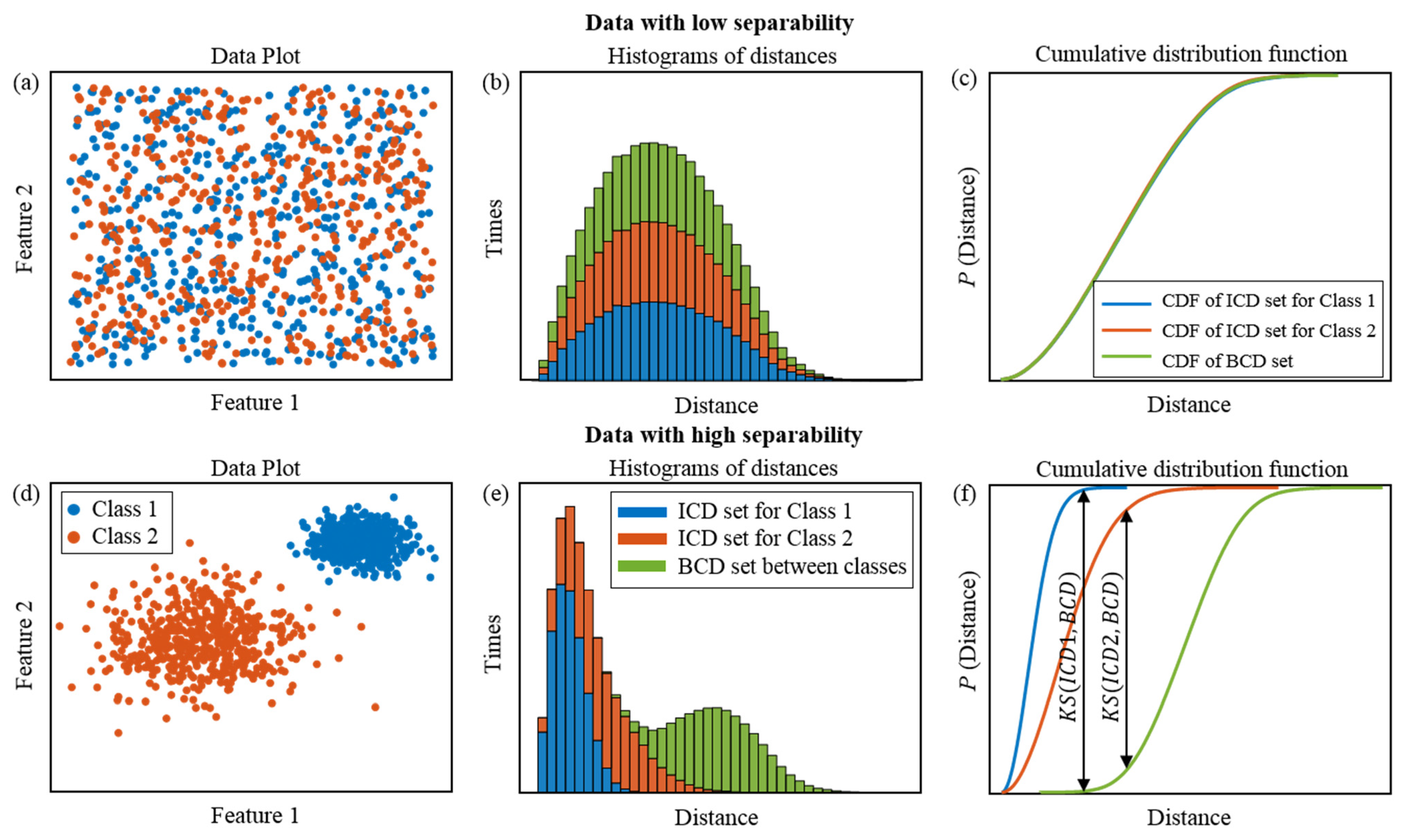
Separability can be defined as the similarity of data distributions. It is natural to understand that the data with the same distribution are hard to separate since it reaches the maximum entropy within any small regions in the space. An example was illustrated in Figure 2: the data in Class 1 and Class 2 in Figure 2a have a very similar distribution and the data points of the two classes are mixed. It is much more challenging to separate the two classes of data correctly. In contrast, the data in Class 1 and Class 2 in Figure 2d have a different distribution in the feature space (positions of the data clusters). It is intuitively much easier to separate the data in Figure 2d than separate the data in Figure 2a.
Guan et al. [33] proposed a distance-based separability index (DSI). It uses the Kolmogorov–Smirnov (KS) distance of the intra-class distance (ICD) sets and the between-class distance (BCD) sets to characterize how the two classes of data are mixed. As shown in Figure 2b,c, the ICD sets and the BCD sets of the low-separable dataset (shown in Figure 2a) have very similar histograms and empirical cumulative distribution functions. As shown in Figure 2e,f, the ICD sets and the BCD sets of the high-separable dataset (shown in Figure 2d) have different histograms and empirical cumulative distribution functions. The KS distance can measure the similarity of two empirical cumulative distribution functions, and its mathematic equation is shown below.
K S ( F 1 , F 2 ) = s u p x | F 1 ( x ) F 2 ( x ) |
where the F 1 ( x ) and F 2 ( x ) are two empirical cumulative distribution functions, and the s u p x | · | is the supremum operator. The KS distance is equal to the maximal vertical distance (see Figure 2f) between two empirical cumulative distribution functions, and its value is between 0 and 1. The closer it is to the unity, the more different the two empirical cumulative distribution functions are.
The DSI is defined as the average of the KS distances between the ICD sets and the BCD sets for each class of data in a dataset.
D S I ( C 1 , C 2 ) = K S ( F I C D 1 , F B C D 1 , 2 ) / 2 + K S ( F I C D 2 , F B C D 1 , 2 ) / 2
where C 1 and C 2 are two classes of dataset, the F I C D 1 , F I C D 2 , and the F B C D 1 , 2 are the empirical cumulative distribution functions of the ICD sets of Class 1 and Class 2, and the BCD sets of Class 1 and Class 2. The Euclidean distance is recommended since the DSI based on Euclidean distance has the best sensitivity to complexity [33]. The value of the DSI is between 0 and 1. The larger the DSI, the better the separability of data.
The DSI can be employed to evaluate the separability of initial features. Supposing the initial feature set contains N -classes, the DSI of the initial feature set can be calculated by following.
(1)
Calculate the N intra-class distance sets for each class: { I C D n } ,   n = 1 , 2 , , N .
(2)
Calculate the N between-class distance sets for each class: { B C D n } ,   n = 1 , 2 , , N . For the n-th class, the between-class distance set is the distances between any two samples in the n -th class and the class other than the n -th class.
(3)
Calculate the DSIs of N classes, and the DSI of the initial feature is the average of the DSIs of N classes.

2.2.2. Distance-Based Transferability Index

In the IFD under variable working conditions, it is well recognized that the feature representation distribution shift between the training dataset and the testing dataset usually leads to a decrease in the diagnosis performance of IFD models. Since the DSI can measure the separability of two empirical cumulative distribution functions, we proposed a data transferability index (DTI) to measure the transferability of initial features on working conditions. The DTI employs the DSI to quantify the separability of initial feature in the testing dataset to the training dataset. The DTI is defined as follows:
D T I ( C t , C s ) = D S I ( C 1 t , C n o t   1 s ) / ( D S I ( C 1 t , C 1 s ) + ε )
where the C t and C s are the training datasets and testing dataset. The C 1 t and C n o t   1 t are the Class 1 and the classes other than Class 1 in the testing dataset. The C 1 s and C n o t   1 s are the Class 1 and the classes other than Class 1 in the training dataset. The ε is a small non-negative number (i.e., 10 6 ) to avoid a denominator of zeros. The D S I ( C 1 t , C 1 s ) measure the separability of same class in the training dataset and the testing dataset. It can be regarded that the smaller the D S I ( C 1 t , C 1 s ) , the closer the feature representation distributions of the same class in the training dataset and the testing dataset are. The D S I ( C 1 t , C n o t   1 s ) measure the separability of different classes in the training dataset and the testing dataset. It can be regarded that the larger the D S I ( C 1 t , C n o t   1 s ) , the further the feature representation distributions of different classes in the training dataset and the testing dataset. Therefore, the larger the D T I ( C t , C s ) , the closer the same classes in the training dataset and the testing dataset and the further the different classes in the training dataset and the testing dataset.
The DTI of testing dataset and training dataset that have the same N classes can be calculated by following:
(1)
Calculate the N intra-class distance sets for each class in the testing dataset and the training dataset: { I C D n t } ,   n = 1 , 2 , , N , and { I C D n s } ,   n = 1 , 2 , , N .
(2)
Calculate the N between-class distance sets for each class in the testing dataset: { B C D n } ,   n = 1 , 2 , , N , For the n -th class, the between-class distance set is the distances between any two samples in the n -th class in testing dataset and the class other than the n -th class in training dataset.
(3)
Calculate the DSIs of each class according to Equation (5) and calculate the ratios of DSIs of each class according to Equation (6). At last, the DTI between the feature set is the average of the DTIs of N classes.

3. Experimental Verification on Gearbox Dataset

3.1. Gearbox Testing Rig and Data Description

The gearbox testing rig shown in Figure 3 consisted of an AC motor, a testing gearbox, a torque sensor, a reducer, and a magnetic brake. An accelerometer is mounted near the bearing house to collect the vibration signals. Five artificial damages (see Figure 3b), including two gear failures: the tooth root cracks of 2 mm in depth (G2) and 4 mm in depth (G4), and three bearing failures: the outer-race fault (OF), the inner-race fault (IF), and the rolling ball fault (BF) were fabricated in the testing gearbox. Together with the Normal condition (NC), six health conditions are contained in the dataset. Vibration signals were collected at 800 rpm (i.e. revolutions per minute), 1000 rpm, and 1200 rpm. The duration of vibration signals for each health condition and speed is 20 s, and the sampling rate is 24,000 Hz.
Fifty samples were made for each health condition and rotating speed, and therefore, 900 samples in total for six health conditions and three rotating speeds. Each sample has a time length of 0.4 s, corresponding to 9600 data points. The detailed information on the gearbox dataset is listed in Table 1.

3.2. MSFED Feature Analysis

An analytic frequency range of 0~12,000 Hz and an analytic scale of 1~6 were used to construct the MSFED-1 feature vector and the MSFED-2 feature map for vibration samples. Besides, four commonly used features, including the Statistical feature, the FFT spectrum feature, the STFT feature, and the OFSCoh feature, were also constructed for the comparison study. The parameter value used in feature construction is presented in Table 2.
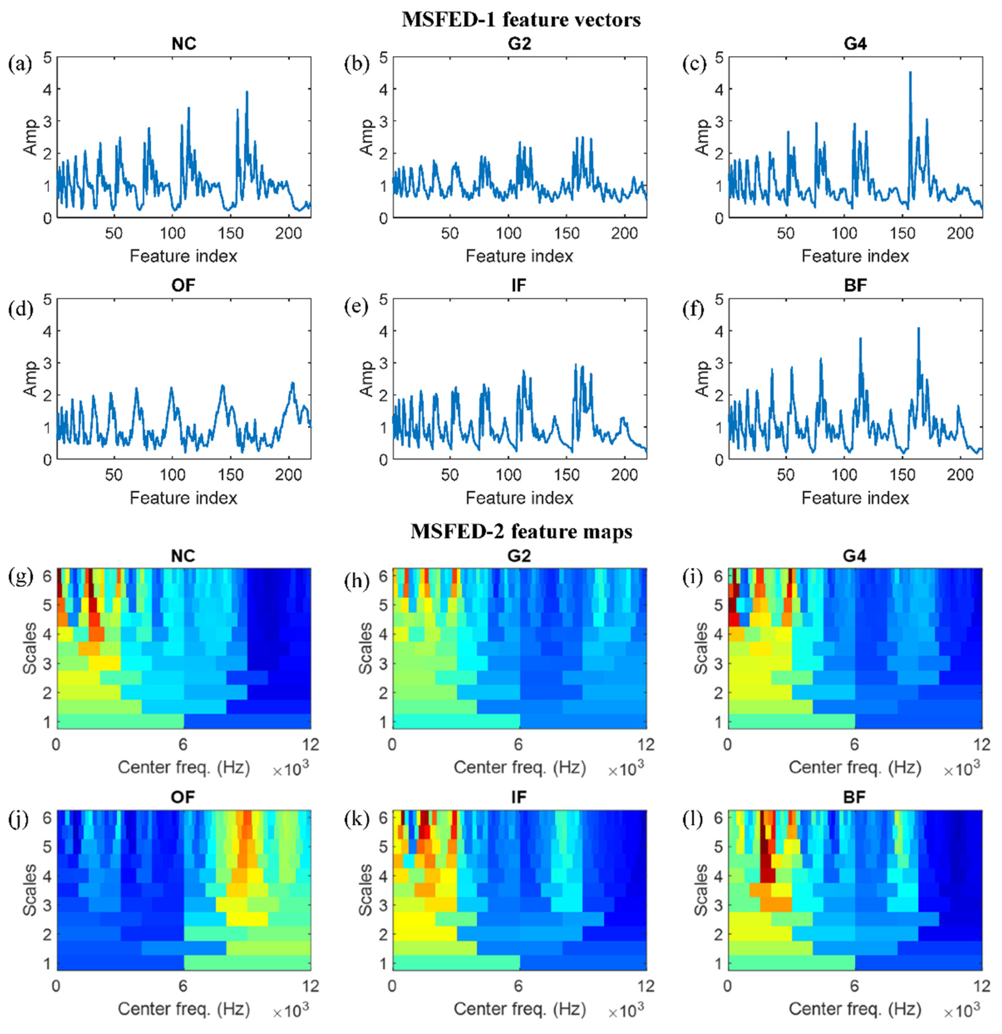
Figure 4 presents the MSFED-1 and MSFED-2 features of samples of six health conditions at the rotating speed of 1000 rpm. As shown in Figure 4a–f, the features on large scales (Scale 5 and 6) provided a more fine-grained characterization of the vibration energy distribution than those on the small scales (Scale 1 and 2). The G2, OF, and IF samples can be intuitively distinguished from the samples of the other three health conditions by observation, as the amplitude of the MSFED-1 feature vectors of the G2, OF, and IF samples are much smaller than the MSFED-1 feature vectors of samples of the other three health conditions. The MSFED-2 feature maps shown in Figure 4g–l appear more distinguishable. As can be observed, the energy density of OF samples is significant in the frequency range of 6000~12,000 Hz, while the energy density of samples in the other five health conditions is significant in the frequency range of 0~6000 Hz. The G2 sample is distinguished from NC, G4, IF, and BF samples, as the energy density of G2 samples is much greater than those of other samples in the frequency range of 9000~12,000 Hz. Even though the MSFED-2 feature maps of NC, G4, and BF samples look similar and are hard to distinguish by observation, they should be separable using some IFD models since these models usually have powerful feature-learning and pattern-recognition capabilities. The feature vectors and maps of the other four preprocessing methods are provided in Appendix A.

3.3. Fault Diagnosis Results Analysis

The superior performance of IFD models depends on a large amount of training data. However, it is often hard to collect a sufficient amount of fault data in practice, particularly for expensive critical machines. Therefore, fault diagnosis using limited training data is prevalent in real industrial applications. Moreover, fault data collected from machines in real industrial environments are often class-imbalanced due to the random occurrence of different faults. This fact appears as a class-imbalanced data problem [34], where the correct diagnosis is much more difficult due to the uneven data distribution of each health condition. Furthermore, machines in industrial applications often work in variable conditions (load and rotating speed), and the diagnosing data sometimes have different working conditions than those of the training data. The diagnosis in variable working conditions is much more complicated than the constant working conditions due to the training and testing data’s distribution divergence caused by the working condition shift. In addition, fault diagnosis in noisy environments has also caught much attention.
Four fault diagnosis tasks were designed using the gearbox dataset, as listed in Table 3. Task T1 is fault diagnosis using limited training samples, in which the training and testing data consist of the first five samples and the last 45 samples of the six health conditions and three rotating speeds. The ratio of training and testing data quantities is 10%, in line with the small sample size scenario. Task T2 is fault diagnosis using class-imbalanced data. The first 25 NC samples, the first 15 G2 and G4 samples, and the first 5 OF, IF, and BF samples are used in the training data. The testing data used the last 25 samples of six health conditions and three rotating speed conditions. Task T3 is fault diagnosis under variable working conditions. The training data consisted of samples in six health conditions at the rotating speed of 1000 rpm, and the testing data consisted of samples in six health conditions at rotating speeds of 800 rpm and 1200 rpm. Task T4 is fault diagnosis under low signal-to-noise ratio conditions. In this task, the white Gaussian noise with an SNR of 0 dB is added to the raw vibration signal to simulate the noisy signal in an industrial environment. The training and testing data consist of the first 25 samples and the last 25 samples of six health conditions and three rotating speed conditions, respectively.
Different IFD models perform differently on datasets and tasks. It is possible for an IFD model to perform well on one dataset or task but sub-optimally on another dataset or task. To thoroughly investigate the performance of the initial features, we test and evaluate the feature on a board set of IFD models. In this paper, seven machine learning algorithms, including the Softmax classifier (Softmax), the K-Nearest Neighbors (KNN), the Support Vector Machine (SVM), the Linear Discriminant Analysis (LDA), the Naive Bayes (NB), the Random Forest (RF), and the Artificial Neural Network (ANN), were used to learn and classify the six initial features. The Principal Component Analysis is used before machine learning algorithms to extract the critical features and reduce the dimensionality of the initial features (except the Statistical feature). The reduction dimensionality of Principal Component Analysis was set to 50 for all initial features, in which the contribution rates were larger than 85%. Moreover, three Convolutional Neural Networks in published papers, including the Yang CNN [35], Chen CNN [25], and Islam CNN [36], are employed to learn and classify the OFSCoh, STFT, and MSFED-2 features. The training and testing processes are repeated five times to reduce the influence of the randomness introduced by the IFD model’s initialization. The hyperparameter setting of IFD models has a significant influence on their diagnosis accuracy. To avoid the randomness caused by the hyperparameter setting of models in the initial feature diagnostic performance comparison, we set a board set of hyperparameter settings for each IFD model and chose the highest diagnostic accuracy to represent the diagnosis performance of the IFD model. Taking the KNN model in Table 4 as an example, the parameters “Nearest neighbor search method”, the “Standardize the features”, the “number of neighbors”, and the “distance metrics” usually have a significant influence on the KNN model’s diagnosis accuracy. We fixed the parameter “Nearest neighbor search method” to “exhaustive search algorithm” and the parameter “Standardize the features” to “True” and tuned the parameter “number of neighbors” in four settings (1, 5, 10, and 15) and tuned the parameter “distance metrics” in three settings (the “Cosine”, the “Euclidean”, and the “Mahalanobis”). There are twelve hyperparameter settings in total, and the highest diagnostic accuracy of the KNN model with these hyperparameter settings was chosen to represent the diagnosis performance of the KNN models. The hyperparameter settings of the ten IFD models are listed in Table 4.
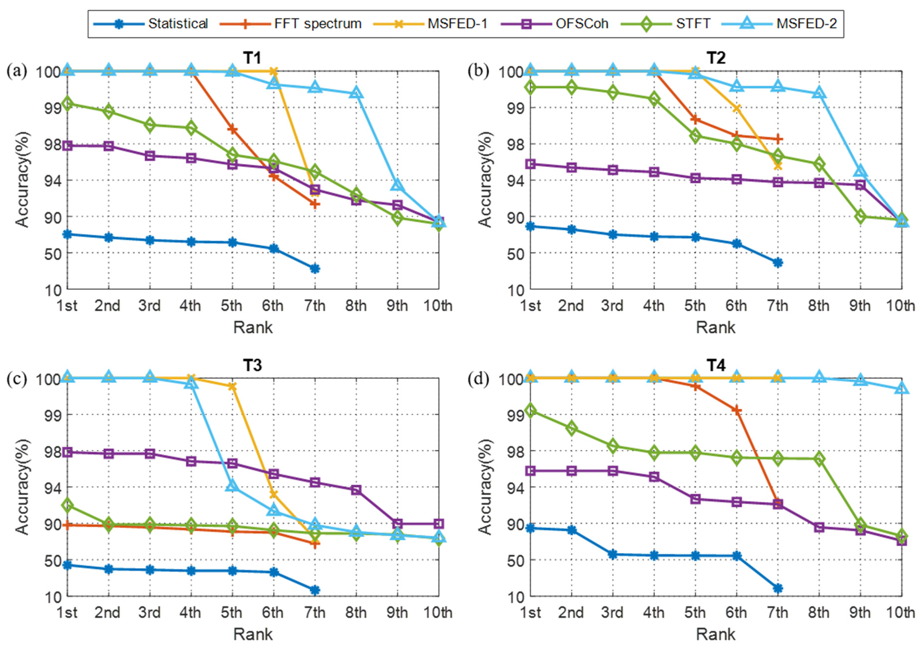
Figure 5 shows the diagnostic accuracies of six features on four diagnosis tasks (see Appendix B for the details of the average and the standard deviation of the diagnostic accuracies of ten IFD models and six features). Each one-dimensional initial feature (i.e., the statistical feature, the FFT spectrum feature, and the MSFED-1 features) has seven diagnostic accuracies. Each two-dimensional initial feature (i.e., the OFSCoh feature, the STFT feature, and the MSFED-2 feature) has ten diagnostic accuracies. These seven (for one-dimensional initial feature) or ten (for two-dimensional initial feature) diagnostic accuracies of each initial feature are arranged in descending order in Figure 5. The abscissa of Figure 5 is the ranking of diagnostic accuracy from the highest (First) to lowest (Seventh or Tenth). Note that the ordinates of the charts were designed to be non-uniform to make all diagnostic accuracy visible and distinguishable. More specifically, the whole range of the ordinate 10.00~100.00 is divided into three intervals: the Interval 10~90, the Interval 90~98, and the Interval 98~100. The Interval 98~100 has a finer resolution than the other two intervals.
As shown in Figure 5a, the FFT spectrum, MSFED-1, and MSFED-2 features achieved the highest diagnostic accuracy on Task T1. The highest diagnostic accuracies of these three features are 100%. In contrast, the STFT and OFSCoh features achieved a moderate diagnostic accuracy, with the highest diagnostic accuracy of 99.11% and 97.78%, respectively. The diagnostic accuracies of the Statistical feature were the lowest among the six features, and its highest diagnostic accuracy is only 70.37%. Similar results can be observed from Figure 5b,d: that the FFT spectrum, MSFED-1, and MSFED-2 features achieved higher diagnostic accuracy than the STFT feature, the OFSCoh feature, much higher than the Statistical feature. In Figure 5c, the MSFED-1 and MSFED-2 features achieved the best diagnostic accuracy among the six initial features. The highest diagnostic accuracies of the MSFED-1 and MSFED-2 features are 100%. In contrast, the FFT spectrum, which achieved high diagnostic accuracy on Tasks T1, T2, and T4, suffered significant performance degradation on Task T3.
The average value of the top-three accuracies of the six initial features is listed in Table 5. We used the average value of the top-three accuracies because we assume users have some expertise in the fault diagnosis and can choose the optimal or suboptimal models for the task at hand. As shown in Table 5, the MSFED-1 and MSFED-2 features achieved 100% diagnostic accuracy on four tasks, far better than the other four features. The FFT spectrum feature achieved 100% diagnostic accuracies on Tasks T1, T2, and T4, while achieving an 86.89% diagnostic accuracy on Task T3. The OFSCoh feature and the STFT feature achieved moderate diagnostic accuracies on those four tasks among the six features. The Statistical features achieved the last diagnostic accuracy among the six features. It can be summarized as follows: (1) The MSFED-1, MSFED-2, and FFT spectrum features performed better than the OFSCoh, STFT features and better than the Statistical features on Tasks T1, T2, and T3. (2) The MSFED-1 and MSFED-2 features performed better than the OFSCoh, STFT, and FFT spectrum features and better than the Statistical feature on Task T3.

3.4. Separability and Transferability Evaluation

The DSIs and DTIs of the six initial features of the gearbox dataset were calculated and listed in Table 6. As shown in Table 6, the DSIs of the MSFED-1, FFT spectrum, and MSFED-2 features are higher than the OFSCoh, STFT, and Statistical features, demonstrating that the MSFED-1, FFT spectrum, and MSFED-2 features have better separability than the OFSCoh, STFT, and Statistical feature. This result is consistent with the diagnostic performance of the six features in Section 3.4 in Tasks T1, T2, and T4. The better the separability of features is, the higher the diagnostic accuracy of features. The average of the DTIs of the OFSCoh is the highest among the six features, indicating that the feature representation distributions of the OFSCoh feature at different speeds have a good similarity. It can be observed from Table 5 that the OFSCoh feature achieved a diagnostic accuracy of 97.72% on Task T3. Although the diagnosis accuracy of the OFSCoh feature is lower than the MSFED-1 and MSFED-2 feature on Task T3, the OFSCoh feature is the only one whose diagnosis accuracy on Task T3 is higher than that on Tasks T1, T2, and T3. The DTIs of the STFT feature and the Statistical features are higher than that of the MSFED-1, and MSFED-2 features. However, due to the low separability of the STFT feature and the Statistical features, the diagnosis accuracies of the STFT feature and the Statistical features are lower than that of the MSFED-1 and MSFED-2 features.

4. Experimental Verification on Bearing Dataset

4.1. Bearing Testing Rig and Data Description

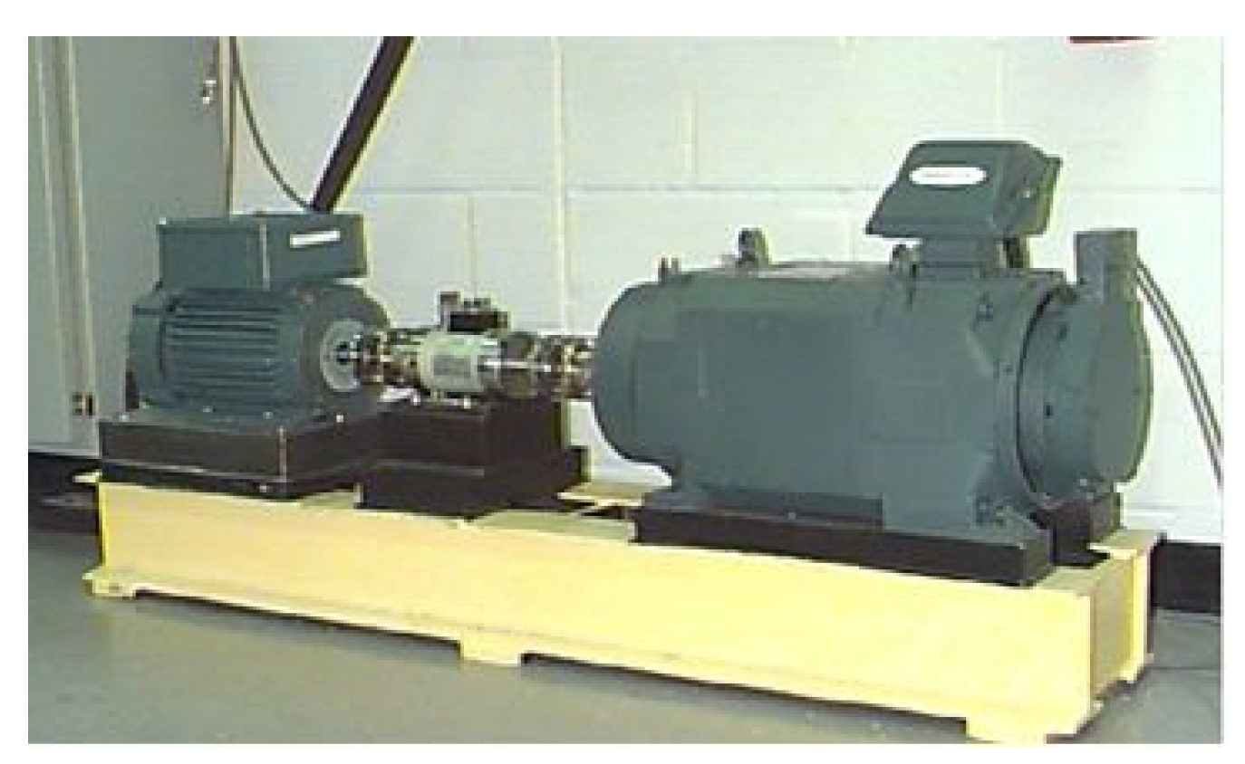
The bearing dataset provided by the Case Western Reserve University (CWRU) [37] was used to verify the effectiveness of the proposed MSFED features. The bearing testing rig in Figure 6 consists of a motor, a torque sensor/encoder, and a dynamometer. The testing bearings are installed at the motor’s driving and fan end. The vibration signal was collected at a sampling rate of 12,000 Hz. In addition to the Normal condition (NC), three failures, including the Outer-race fault (OF), the Inner-race fault (IF), and the Ball fault (BF), had been fabricated on the testing bearing. Each failure contains three severities with failure diameters of 7 mils, 14 mils, and 21 mils (1 mil = 0.001 inch). For each health condition, the vibration signals were collected under four working conditions with load and speed of 0 hp/1797 rpm, 1 hp/1772 rpm, 2 hp/1750 rpm, 3 hp/1730 rpm. Therefore, there are, in total, ten health conditions and four operating conditions in the bearing dataset.
The vibration signals collected at the driving end of the motor are used to make datasets. Fifty samples were made for each health condition with each load condition. As a result, 2000 samples were made for ten health conditions and four load conditions. The samples have a time length of 0.2 s, corresponding to 2400 data points. The details of bearing datasets are shown in Table 7.

4.2. MSFED Feature Analysis

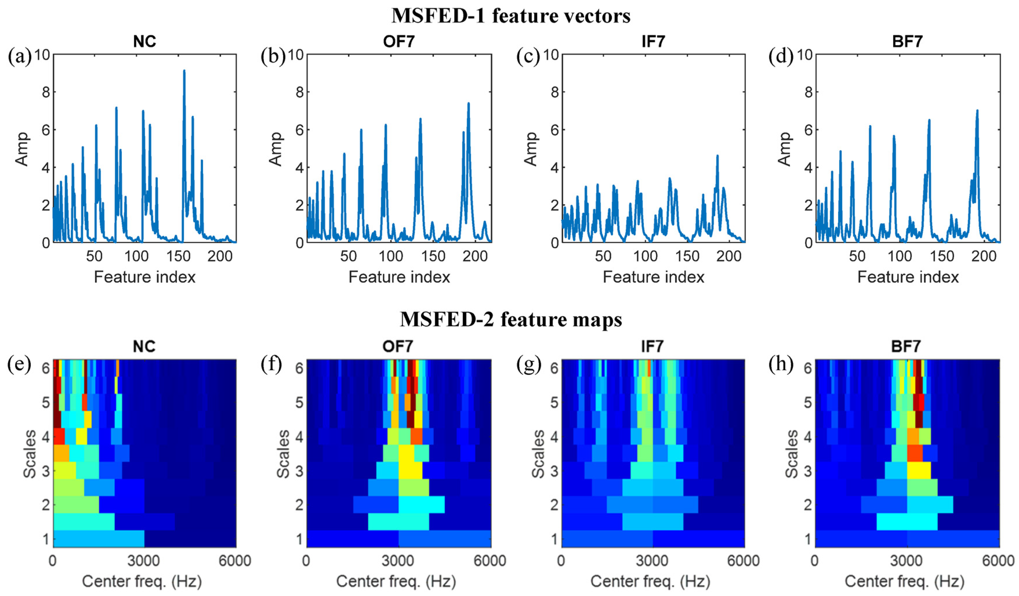
The MSFED-1 feature vectors and the MSFED-2 feature maps of the NC, OF7, IF7, and BF7 samples at 1 hp load are presented in Figure 7. The analytic frequency range is 0~6000 Hz, and the analytic scale is 1~6. As shown in Figure 7, the IF7 samples are easily distinguished from samples of the other three health conditions, as the amplitude of the MSFED-1 feature vector of the IF7 samples is much smaller than those of the other three health conditions. It is also observed from the MSFED feature maps in Figure 7g that the vibration energy of IF7 samples dispersed in a wider frequency range compared to that of samples of the other three health conditions. The NC sample distinguishes from the OF 7 and BF7 samples as its energy density in 0~3000 Hz is much greater. The feature vectors and maps of the other four preprocessing methods are provided in Appendix A.

4.3. Fault Diagnosis Results Analysis

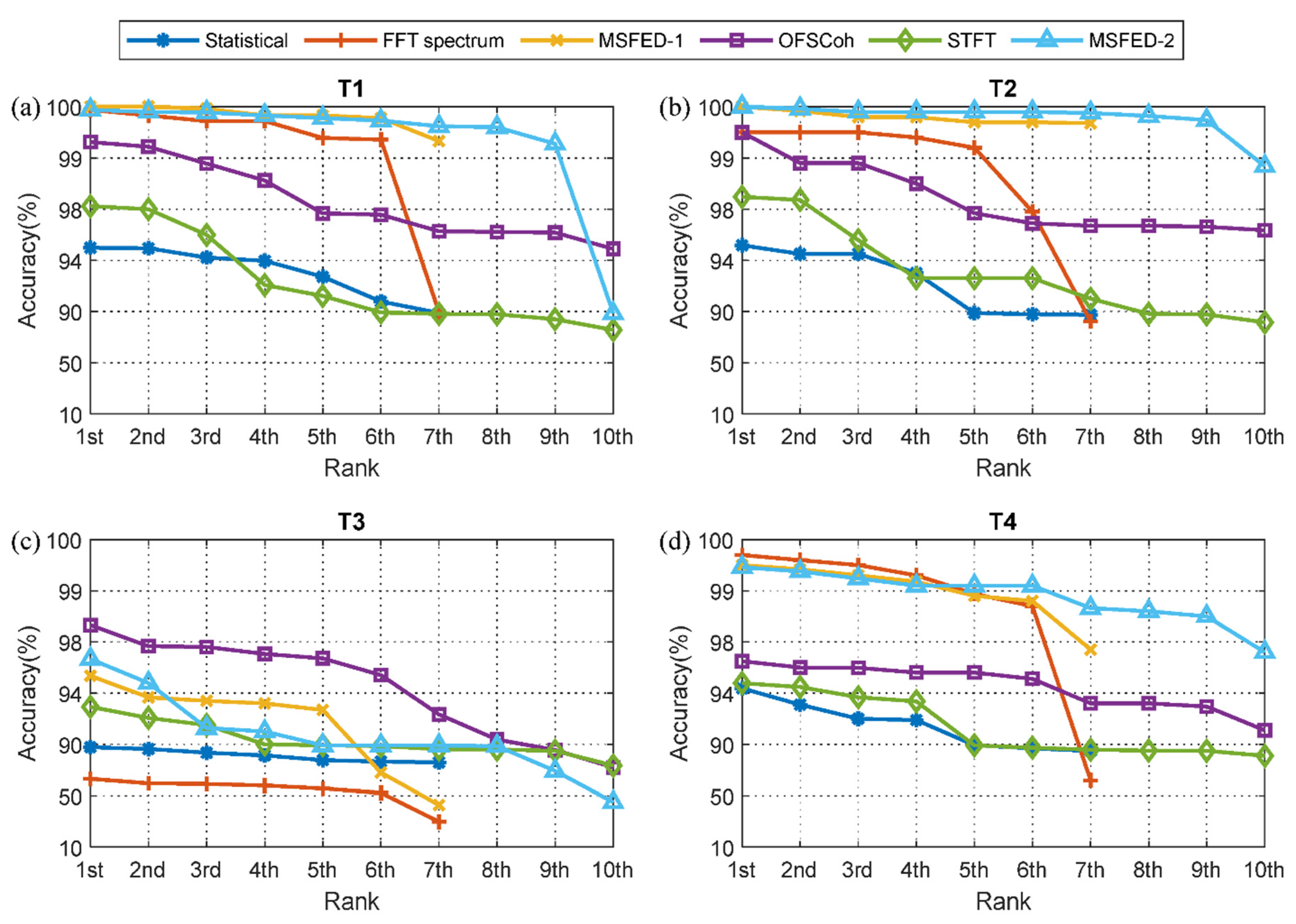
The fault diagnosis scenarios in Section 3.3 are used again in the bearing fault diagnosis. Four tasks were designed using the CWRU bearing dataset. As shown in Table 8, the training and testing data of Task T1 consist of the first five and the last 45 samples of ten health conditions and four load conditions. In Task T2, the training data consist of the first 25 NC samples, the first 15 OF7, OF14, and OF21 samples, the first 10 IF7, IF14, and IF21 samples, and the first 5 BF7 and BF14 and BF21 samples. The testing data consist of the last 25 samples of all health conditions. Task T3 is used to simulate a diagnosis in variable load conditions. The training data use all samples in the 0 hp load, and the testing data use all samples in the 1 hp, 2 hp, and 3 hp loads. Task T4 is used to simulate the diagnosis under low SNR conditions. The white Gaussian noise with 0 dB is added to the raw vibration samples, and the training data and testing data consist of the first 25 and the last 25 samples of all health conditions and load conditions. The IFD models and hyperparameter settings used in the gearbox case study in Section 3.3 are used for the bearing fault diagnosis.
Figure 8 shows the diagnostic accuracies of six features on four diagnosis tasks (see Appendix B for the details of the average and the standard deviation of the diagnostic accuracies of ten IFD models and six features). As can be observed from Figure 8a,b,d, the MSFED-1, MSFED-2, and the FFT spectrum features achieved higher diagnostic accuracies than the OFSCoh, STFT, and Statistical features on tasks T1, T2, and T3. It is inferred that the MSFED-1, MSFED-2, and FFT spectrum features are more easily classified by most IFD models than the OFSCoh, STFT, and Statistical features. In Task T3, the OFSCoh feature achieved the highest diagnostic accuracy among the six features, as depicted in Figure 8c. It can also be observed that the MSFED-1 and MSFED-2 features achieved the second-highest and the third-highest diagnostic accuracy on Task T3. In contrast, the FFT spectrum feature achieved the lowest diagnostic accuracy on Task T3.
The average value of the top-three accuracies of the six initial features is listed in Table 9. As shown in Table 9, the diagnostic accuracies of MSFED-1, MSFED-2, and FFT spectral features on tasks T1, T2, and T4 are all higher than 99.30%, which is superior to the other three features. In contrast, the OFSCoh achieved the highest diagnostic accuracy of 97.87% on Task 3, higher than the 94.24% and 94.14% diagnostic accuracies of the MSFED-2 and MSFED-1 features. The results can be summarized as follows: (1) The FFT spectrum, MSFED-1, and MSFED-2, and features performed better than the OFSCoh, STFT features, and better than the Statistical features on Tasks T1, T2, and T4. (2) The OFSCoh feature performed better than the MSFED-1 and MSFED-2 features, the STFT, FFT spectrum features, and the Statistical feature on Task T3.

4.4. Separability and Transferability Evaluation

The DSIs and DTIs of the six initial features of the bearing dataset were calculated and listed in Table 10. As shown in Table 6, the DSIs of the MSFED-1, FFT spectrum, and MSFED-2 features are higher than the OFSCoh feature and much higher than STFT and Statistical features, demonstrating that the separability of MSFED-1, FFT spectrum, and MSFED-2 features are better than that of the OFSCoh and far better than that of the STFT, and Statistical feature. The separability evaluation result is consistent with the diagnostic performance of the six features in Section 4.4 in Tasks T1, T2, and T4, and as can be seen from Table 9, the diagnosis accuracy of the MSFED-1, FFT spectrum, and MSFED-2 features are higher than that of the STFT feature, and higher than that of the STFT and Statistical features.
The DTIs of six features on 0→1 hp are higher than 0→2 hp and higher than 0→3 hp (except for the DTIs of the FFT spectrum feature), which indicates that the transferability of features on 0→1 hp is better than 0→2 hp and better than 0→3 hp. The results were in agreement with the intuitive understanding that the greater the variation between working conditions, the lower the data distribution similarity, as well as the data’s transferability. Meanwhile, the diagnostic accuracy results in the variable load conditions in papers [38,39,40] are consistent with the trend of DTIs evaluation results. In those papers, the diagnostic accuracy of 0→1 hp is higher than that of 0→2 hp and 0→3 hp, proving the effectiveness of the developed data transferability metric. It can also be observed that the MSFED-1 and MSFED-2 features have higher DTIs than the FFT spectrum feature on the bearing dataset. It is in agreement with the diagnosis result that the MSFED-1 and MSFED-2 features achieved much higher diagnostic accuracy than the FFT spectrum feature on Task T3. In addition, the DTIs of Statistical features, the OFSCoh feature, and the STFT features are higher than those of the other three features. However, the DTIs of features should not be wholly equated with their diagnostic performance on Task T3. It is because the diagnostic ability of features on the variable working condition scenarios not only relates to the transferability of the features on working conditions but also depends on the separability of features themselves.

5. Conclusions

This paper proposed a MSFED feature for vibration-based intelligent fault diagnosis of rotating machines. The MSFED feature revealed the vibration energy distribution pattern of rotating machines, and its one-dimensional format (MSFED-1) and two-dimensional format (MSFED-2) make it usable for most intelligent fault-diagnosis models. Experimental validation on the gearbox and bearing datasets verified the effectiveness of the MSFED feature. Furthermore, the separability and the transferability of the MSFED features were studied using a model-independent method for the first time. The key findings of this paper are listed as follows.
(1)
The MSFED feature revealed the vibration energy distribution pattern and generated discriminative feature vectors and maps for different fault types. In gearbox fault diagnosis, the MSFED features achieved accuracy (average accuracy of top three) of 100% in all four tasks, higher than the Statistics feature, FFT spectrum feature, STFT feature, and OFSCoh feature. In bearing fault diagnosis, the MSFED features achieved accuracies of 99.99% (MSFED-1) on the limited training data fault-diagnosis task, 99.95% (MSFED-2) on the class-imbalanced data fault-diagnosis task, 94.24% (MSFED-2) on the variable-load data fault-diagnosis task, and 99.41% (MSFED-1) on the low signal-to-noise ratio data fault-diagnosis task. The accuracy of the MSFED feature is higher than the other four features on the limited training data fault-diagnosis task and the class-imbalanced data fault-diagnosis task, while lower than the OFSCoh feature on the variable-load data fault-diagnosis task (97.87%), and a little lower than the FFT Spectrum feature on the low signal-to-noise ratio data fault-diagnosis task (99.60%).
(2)
The separability and transferability evaluation results of the initial features are in good agreement with the diagnostic performance of initial features. The data separability index s of the MSFED features are a little lower than that of the FFT spectrum feature, but higher than that of the Statistics feature, the OFSCoh feature, and the STFT feature, on the gearbox dataset and bearing dataset. The data transferability index s of the MSFED features is lower than the Statistics feature, the OFSCoh feature, and the STFT feature, but higher than the FFT spectrum feature.
The MSFED feature proposed in this paper provided a promising initial feature for intelligent fault diagnosis of rotating machines. In addition, the model-independent initial feature quality evaluation method offers a new means of quality evaluation in feature development without complex diagnosis-model construction and time-consuming model training.

Author Contributions

Conceptualization, C.W.; Data curation, Q.Z. and X.Z.; Formal analysis, X.Z.; Funding acquisition, C.W.; Investigation, Q.Z.; Methodology, C.W.; Project administration, C.W.; Software, X.Z.; Supervision, C.W.; Visualization, Q.Z.; Writing—original draft, Q.Z. All authors have read and agreed to the published version of the manuscript.

Funding

This research was funded by key research and development project of Hubei province, grant number 2020BAB033.

Institutional Review Board Statement

Not applicable.

Informed Consent Statement

Not applicable.

Data Availability Statement

The data sets generated and/or analyzed during the current study are available from the corresponding author on reasonable request.

Conflicts of Interest

The authors declare no conflict of interest.

Appendix A. Features of the Gearbox Dataset and Bearing Dataset
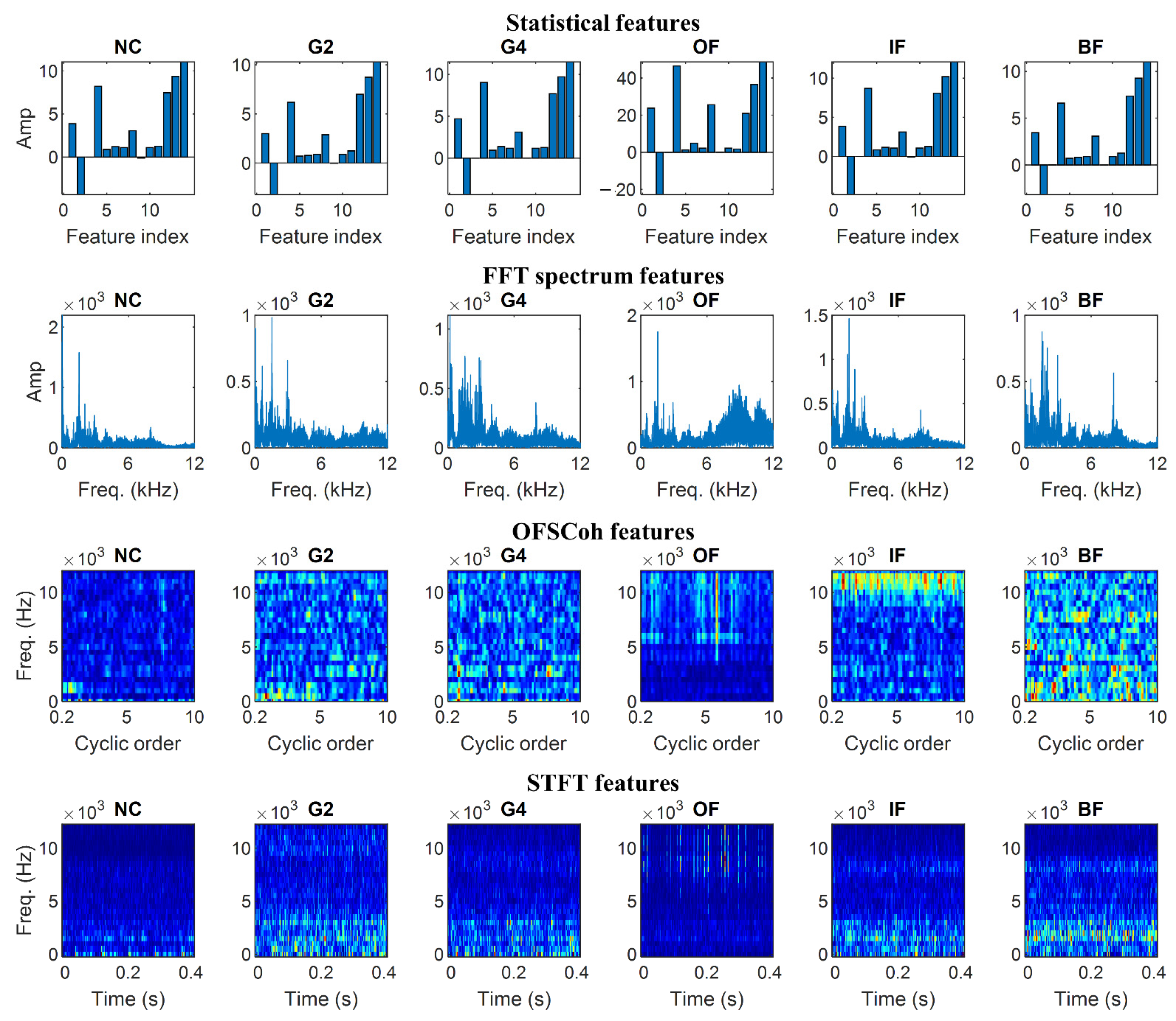
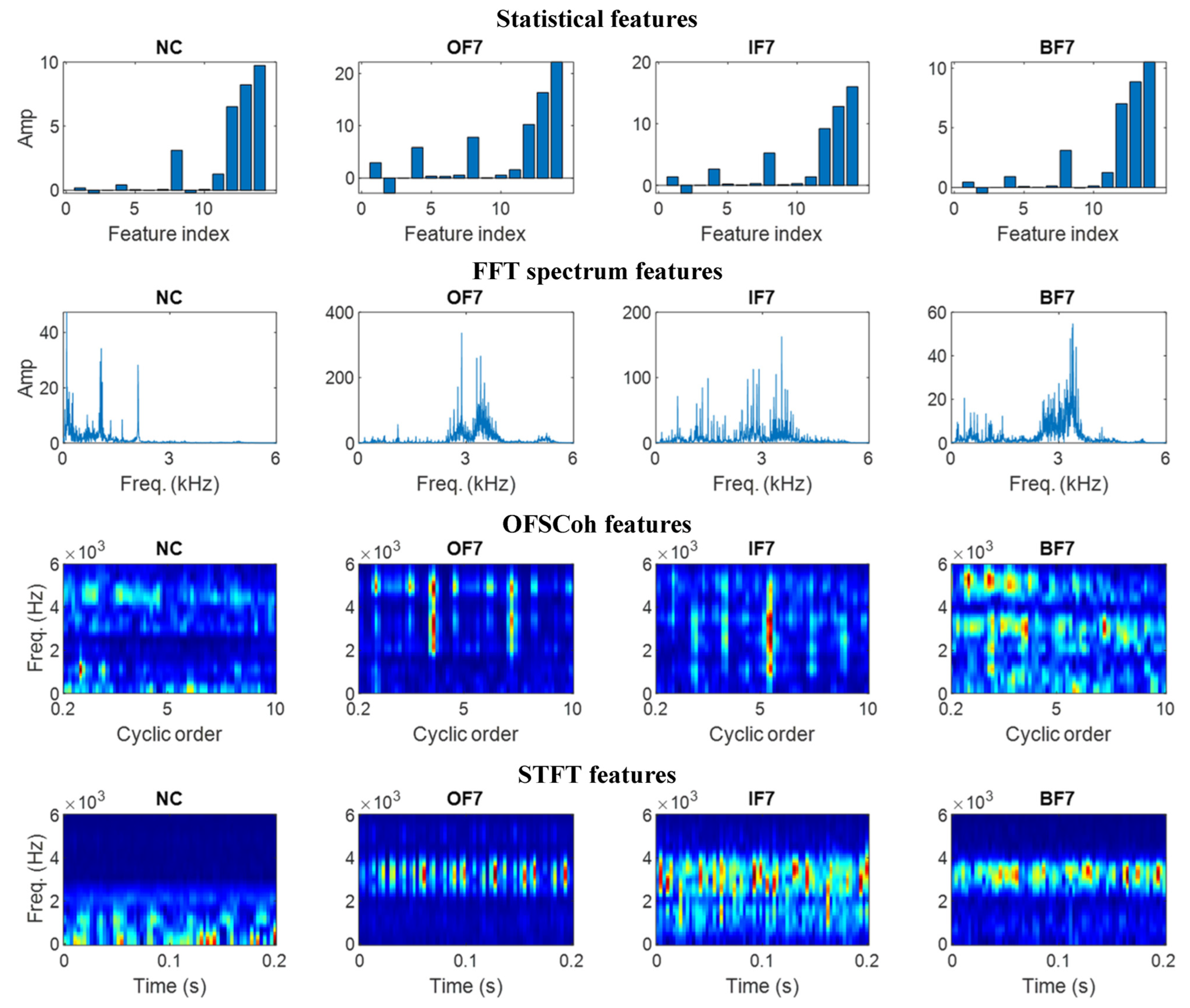
Figure A1. The Statistical, FFT spectrum, OFSCoh, and the STFT features of gearbox dataset at 1000 rpm.
Machines 10 00743 g0a1
Figure A2. The Statistical, FFT spectrum, OFSCoh, and the STFT features of bearing dataset at 1 hp.
Machines 10 00743 g0a2

Appendix B. Diagnostic Accuracies of the Six Features and the Ten IFD Models

Table A1. The diagnostic accuracies on gearbox dataset.
FeaturesIFD ModelsAccuracy (%)
T1T2T3T4
StatisticalSoftmax54.57 ± 0.0060.00 ± 0.0036.50 ± 0.0054.22 ± 0.00
KNN61.36 ± 0.0070.00 ± 0.0044.33 ± 0.0055.78 ± 0.00
SVM32.47 ± 0.0039.11 ± 0.0016.67 ± 0.0018.67 ± 0.00
LDA62.10 ± 0.0067.11 ± 0.0038.00 ± 0.0054.67 ± 0.00
NB63.83 ± 0.0067.78 ± 0.0038.00 ± 0.0054.44 ± 0.00
RF70.37 ± 1.4079.11 ± 0.4239.87 ± 0.3484.67 ± 0.37
ANN66.79 ± 3.0175.60 ± 1.7739.10 ± 11.2282.53 ± 1.84
FFT spectrumSoftmax100.00 ± 0.00100.00 ± 0.0085.50 ± 0.00100.00 ± 0.00
KNN98.40 ± 0.0098.22 ± 0.0088.00 ± 0.0099.78 ± 0.00
SVM94.44 ± 0.00100.00 ± 0.0079.83 ± 0.0092.22 ± 0.00
LDA100.00 ± 0.00100.00 ± 0.0083.33 ± 0.00100.00 ± 0.00
NB91.36 ± 0.0098.67 ± 0.0067.67 ± 0.0099.11 ± 0.00
RF100.00 ± 0.0098.13 ± 0.3980.87 ± 0.69100.00 ± 0.00
ANN100.00 ± 0.00100.00 ± 0.0087.17 ± 0.00100.00 ± 0.00
MSFED-1Softmax100.00 ± 0.00100.00 ± 0.00100.00 ± 0.00100.00 ± 0.00
KNN92.59 ± 0.0095.56 ± 0.0073.00 ± 0.00100.00 ± 0.00
SVM100.00 ± 0.00100.00 ± 0.00100.00 ± 0.00100.00 ± 0.00
LDA100.00 ± 0.00100.00 ± 0.00100.00 ± 0.00100.00 ± 0.00
NB100.00 ± 0.00100.00 ± 0.0093.17 ± 0.00100.00 ± 0.00
RF100.00 ± 0.0098.98 ± 0.2799.77 ± 0.20100.00 ± 0.00
ANN100.00 ± 0.00100.00 ± 0.00100.00 ± 0.00100.00 ± 0.00
OFSCohSoftmax97.78 ± 0.0095.78 ± 0.0097.83 ± 0.0095.11 ± 0.00
KNN92.96 ± 0.0094.22 ± 0.0093.67 ± 0.0092.67 ± 0.00
SVM96.67 ± 0.0093.78 ± 0.0097.67 ± 0.0095.78 ± 0.00
LDA96.42 ± 0.0094.89 ± 0.0096.83 ± 0.0095.78 ± 0.00
NB83.83 ± 0.0083.56 ± 0.0094.50 ± 0.0070.89 ± 0.00
RF95.73 ± 0.6293.69 ± 0.6196.60 ± 0.3192.09 ± 0.56
ANN97.75 ± 0.0595.11 ± 0.0097.67 ± 0.0095.78 ± 0.00
ChenCNN95.31 ± 0.6395.38 ± 1.2695.43 ± 2.1392.36 ± 1.38
YangCNN91.78 ± 1.1093.47 ± 1.6589.50 ± 4.4785.60 ± 2.06
IslamCNN91.26 ± 1.5894.09 ± 1.4089.47 ± 2.2682.27 ± 2.60
STFTSoftmax96.79 ± 0.0098.22 ± 0.0087.00 ± 0.0097.78 ± 0.00
KNN88.52 ± 0.0086.22 ± 0.0079.00 ± 0.0088.22 ± 0.00
SVM94.94 ± 0.0098.00 ± 0.0087.83 ± 0.0097.11 ± 0.00
LDA98.52 ± 0.0099.56 ± 0.0092.00 ± 0.0097.78 ± 0.00
NB81.73 ± 0.0090.00 ± 0.0078.83 ± 0.0076.00 ± 0.00
RF96.10 ± 0.6595.78 ± 0.6382.47 ± 6.0298.13 ± 0.30
ANN98.89 ± 0.0099.56 ± 0.0088.80 ± 0.1997.16 ± 0.09
ChenCNN99.11 ± 0.3299.42 ± 0.2388.70 ± 5.4198.62 ± 0.65
YangCNN92.40 ± 3.2096.67 ± 1.3677.63 ± 6.4097.24 ± 0.52
IslamCNN98.44 ± 0.7099.24 ± 0.4473.30 ± 3.6499.11 ± 0.54
MSFED-2Softmax100.00 ± 0.00100.00 ± 0.0099.83 ± 0.00100.00 ± 0.00
KNN93.33 ± 0.0094.89 ± 0.0074.17 ± 0.00100.00 ± 0.00
SVM83.33 ± 0.0083.33 ± 0.00100.00 ± 0.00100.00 ± 0.00
LDA100.00 ± 0.00100.00 ± 0.00100.00 ± 0.00100.00 ± 0.00
NB99.38 ± 0.00100.00 ± 0.0091.33 ± 0.00100.00 ± 0.00
RF100.00 ± 0.0099.38 ± 0.2987.97 ± 3.05100.00 ± 0.00
ANN100.00 ± 0.00100.00 ± 0.00100.00 ± 0.00100.00 ± 0.00
ChenCNN99.98 ± 0.0599.91 ± 0.1894.03 ± 3.52100.00 ± 0.00
YangCNN99.53 ± 0.3099.56 ± 0.2880.33 ± 5.1699.69 ± 0.23
IslamCNN99.63 ± 0.4199.56 ± 0.5876.83 ± 10.1399.91 ± 0.11
Table A2. The diagnostic accuracies on bearing dataset.
FeaturesIFD ModelsAccuracy (%)
T1T2T3T4
StatisticalSoftmax90.78 ± 0.0087.50 ± 0.0076.47 ± 0.0089.30 ± 0.00
KNN88.89 ± 0.0088.80 ± 0.0086.33 ± 0.0084.80 ± 0.00
SVM94.94 ± 0.0094.50 ± 0.0077.67 ± 0.0086.90 ± 0.00
LDA94.22 ± 0.0094.50 ± 0.0081.27 ± 0.0092.00 ± 0.00
NB92.72 ± 0.0093.00 ± 0.0075.93 ± 0.0093.10 ± 0.00
RF94.99 ± 0.0695.18 ± 0.0787.71 ± 0.6994.38 ± 0.28
ANN93.96 ± 0.4987.92 ± 0.5283.44 ± 0.3591.90 ± 0.11
FFT spectrumSoftmax99.83 ± 0.0099.50 ± 0.0055.53 ± 0.0099.60 ± 0.00
KNN99.39 ± 0.0099.40 ± 0.0057.87 ± 0.0098.70 ± 0.00
SVM89.61 ± 0.0082.30 ± 0.0052.20 ± 0.0061.90 ± 0.00
LDA99.72 ± 0.0099.20 ± 0.0059.07 ± 0.0099.30 ± 0.00
NB99.72 ± 0.0099.50 ± 0.0029.67 ± 0.0099.50 ± 0.00
RF99.36 ± 0.1597.80 ± 0.1163.11 ± 1.1298.94 ± 0.20
ANN99.94 ± 0.0099.50 ± 0.4759.57 ± 4.6899.70 ± 0.00
MSFED-1Softmax99.83 ± 0.0099.80 ± 0.0093.40 ± 0.0098.80 ± 0.00
KNN99.33 ± 0.0099.70 ± 0.0068.00 ± 0.0097.40 ± 0.00
SVM99.78 ± 0.0099.70 ± 0.0093.20 ± 0.0098.90 ± 0.00
LDA100.00 ± 0.00100.00 ± 0.0093.67 ± 0.0099.30 ± 0.00
NB100.00 ± 0.0099.80 ± 0.0042.80 ± 0.0099.50 ± 0.00
RF99.83 ± 0.0599.68 ± 0.0492.68 ± 0.8099.18 ± 0.25
ANN99.96 ± 0.0499.92 ± 0.0795.36 ± 0.7399.42 ± 0.10
OFSCohSoftmax98.89 ± 0.0098.90 ± 0.0097.07 ± 0.0095.60 ± 0.00
KNN96.22 ± 0.0096.70 ± 0.0092.33 ± 0.0091.10 ± 0.00
SVM98.56 ± 0.0098.50 ± 0.0097.67 ± 0.0096.50 ± 0.00
LDA99.22 ± 0.0098.90 ± 0.0098.33 ± 0.0096.00 ± 0.00
NB94.89 ± 0.0096.90 ± 0.0071.93 ± 0.0093.20 ± 0.00
RF97.57 ± 0.2396.62 ± 0.2696.72 ± 0.7395.12 ± 0.25
ANN99.31 ± 0.0499.50 ± 0.0097.61 ± 0.0395.98 ± 0.12
ChenCNN97.67 ± 0.3497.68 ± 0.3895.41 ± 0.8895.60 ± 0.30
YangCNN96.28 ± 0.5396.70 ± 0.4185.60 ± 1.6992.96 ± 0.59
IslamCNN96.17 ± 0.8596.36 ± 0.8590.37 ± 1.6993.20 ± 0.74
STFTSoftmax84.00 ± 0.0087.80 ± 0.0086.20 ± 0.0085.10 ± 0.00
KNN75.56 ± 0.0081.50 ± 0.0073.40 ± 0.0081.00 ± 0.00
SVM88.17 ± 0.0091.00 ± 0.0084.87 ± 0.0084.90 ± 0.00
LDA91.22 ± 0.0092.60 ± 0.0092.93 ± 0.0089.20 ± 0.00
NB87.94 ± 0.0092.60 ± 0.0085.93 ± 0.0087.40 ± 0.00
RF89.31 ± 0.6488.32 ± 1.2288.72 ± 0.4485.78 ± 0.72
ANN92.07 ± 0.0492.60 ± 0.2489.35 ± 0.9293.68 ± 0.27
ChenCNN98.00 ± 0.7398.18 ± 0.4491.51 ± 0.9594.48 ± 0.63
YangCNN95.99 ± 0.2495.58 ± 0.6589.92 ± 1.2793.36 ± 0.51
IslamCNN98.06 ± 0.9398.24 ± 0.5292.07 ± 2.2094.78 ± 0.64
MSFED-2Softmax99.89 ± 0.0099.90 ± 0.0091.27 ± 0.0098.50 ± 0.00
KNN99.28 ± 0.0099.90 ± 0.0069.27 ± 0.0097.20 ± 0.00
SVM88.56 ± 0.0099.90 ± 0.0089.13 ± 0.0098.60 ± 0.00
LDA99.94 ± 0.00100.00 ± 0.0096.67 ± 0.0099.10 ± 0.00
NB99.83 ± 0.0099.90 ± 0.0044.93 ± 0.0099.10 ± 0.00
RF99.90 ± 0.0499.96 ± 0.0594.79 ± 0.6099.10 ± 0.11
ANN100.00 ± 0.00100.00 ± 0.0095.07 ± 3.1999.64 ± 0.05
ChenCNN99.78 ± 0.0999.88 ± 0.0491.01 ± 1.3399.46 ± 0.12
YangCNN99.73 ± 0.0698.84 ± 0.7689.07 ± 2.7098.66 ± 0.32
IslamCNN99.60 ± 0.1999.82 ± 0.1289.19 ± 2.0299.24 ± 0.21

References

  1. Vishwakarma, M.; Purohit, R.; Harshlata, V.; Rajput, P. Vibration analysis & condition monitoring for rotating machines: A review. In Proceedings of the 5th International Conference on Materials Processing and Characterization (ICMPC), Gokaraju Rangaraju Institute of Engineering and Technology, Hyderabad, India, 12–13 March 2016; pp. 2659–2664. [Google Scholar]
  2. Guan, S.Y.; Huang, D.R.; Guo, S.H.; Zhao, L.; Chen, H.T. An Improved Fault Diagnosis Approach Using LSSVM for Complex Industrial Systems. Machines 2022, 10, 443. [Google Scholar] [CrossRef]
  3. Peng, Y.W.; Ma, X.H. A Fault Diagnosis Method of Rolling Bearings Based on Parameter Optimization and Adaptive Generalized S-Transform. Machines 2022, 10, 207. [Google Scholar] [CrossRef]
  4. Raouf, I.; Lee, H.; Kim, H.S. Mechanical fault detection based on machine learning for robotic RV reducer using electrical current signature analysis: A data-driven approach. J. Comput. Des. Eng. 2022, 9, 417–433. [Google Scholar] [CrossRef]
  5. Rohan, A.; Raouf, I.; Kim, H.S. Rotate Vector (RV) Reducer Fault Detection and Diagnosis System: Towards Component Level Prognostics and Health Management (PHM). Sensors 2020, 20, 6845. [Google Scholar] [CrossRef]
  6. Gültekin, Ö.; Cinar, E.; Özkan, K.; Yazıcı, A. Multisensory data fusion-based deep learning approach for fault diagnosis of an industrial autonomous transfer vehicle. Expert Syst. Appl. 2022, 200, 117055. [Google Scholar] [CrossRef]
  7. He, Q. Vibration signal classification by wavelet packet energy flow manifold learning. J. Sound Vib. 2013, 332, 1881–1894. [Google Scholar] [CrossRef]
  8. Chen, X.; Yang, Y.; Cui, Z.; Shen, J. Vibration fault diagnosis of wind turbines based on variational mode decomposition and energy entropy. Energy 2019, 174, 1100–1109. [Google Scholar] [CrossRef]
  9. Javorskyj, I.; Matsko, I.; Yuzefovych, R.; Lychak, O.; Lys, R. Methods of Hidden Periodicity Discovering for Gearbox Fault Detection. Sensors 2021, 21, 6138. [Google Scholar] [CrossRef]
  10. Aijun, H.; Jianfeng, L.; Shangfei, S.; Ling, X. A Novel Approach of Impulsive Signal Extraction for Early Fault Detection of Rolling Element Bearing. Shock Vib. 2017, 2017, 9375491. [Google Scholar] [CrossRef]
  11. Peng, C.; Bo, L. Vibration Signal Analysis of Journal Bearing Supported Rotor System by Cyclostationarity. Shock Vib. 2014, 2014, 952958. [Google Scholar] [CrossRef] [Green Version]
  12. Prasad, A.; Dantreliya, C.; Chande, M.; Chauhan, V.; Rai, A. An intelligent fault diagnosis framework based on piecewise aggregate approximation, statistical moments, and sparse autoencoder. Proc. Inst. Mech. Eng. Part O-J. Risk Reliab. 2022. [Google Scholar] [CrossRef]
  13. Li, Y.; Wang, X.; Liu, Z.; Liang, X.; Si, S. The Entropy Algorithm and Its Variants in the Fault Diagnosis of Rotating Machinery: A Review. IEEE Access 2018, 6, 66723–66741. [Google Scholar] [CrossRef]
  14. Zhang, X.; Cong, Y.; Yuan, Z.; Zhang, T.; Bai, X.; Rosso, C. Early Fault Detection Method of Rolling Bearing Based on MCNN and GRU Network with an Attention Mechanism. Shock Vib. 2021, 2021, 6660243. [Google Scholar] [CrossRef]
  15. Nguyen, V.H.; Cheng, J.S.; Yu, Y.; Thai, V.T. An architecture of deep learning network based on ensemble empirical mode decomposition in precise identification of bearing vibration signal. J. Mech. Sci. Technol. 2019, 33, 41–50. [Google Scholar] [CrossRef]
  16. Xu, Y.H.; Li, S.F.; Jiang, W.; Liu, W.; Zhao, K.J. A progressive fault diagnosis method for rolling bearings based on VMD energy entropy and a deep adversarial transfer network. Meas. Sci. Technol. 2022, 33, 095003. [Google Scholar] [CrossRef]
  17. Kumar, A.; Tang, H.S.; Vashishtha, G.; Xiang, J.W. Noise subtraction and marginal enhanced square envelope spectrum (MESES) for the identification of bearing defects in centrifugal and axial pump. Mech. Syst. Signal Process. 2022, 165, 108366. [Google Scholar] [CrossRef]
  18. Puche-Panadero, R.; Martinez-Roman, J.; Sapena-Bano, A.; Burriel-Valencia, J.; Pineda-Sanchez, M.; Perez-Cruz, J.; Riera-Guasp, M. New method for spectral leakage reduction in the FFT of stator currents: Application to the diagnosis of bar breakages in cage motors working at very low slip. IEEE Trans. Instrum. Meas. 2021, 70, 1–11. [Google Scholar] [CrossRef]
  19. Tao, H.F.; Wang, P.; Chen, Y.Y.; Stojanovic, V.; Yang, H.Z. An unsupervised fault diagnosis method for rolling bearing using STFT and generative neural networks. J. Frankl. Inst.-Eng. Appl. Math. 2020, 357, 7286–7307. [Google Scholar] [CrossRef]
  20. Xi, W.K.; Li, Z.X.; Tian, Z.; Duan, Z.H. A feature extraction and visualization method for fault detection of marine diesel engines. Measurement 2018, 116, 429–437. [Google Scholar] [CrossRef]
  21. Hu, M.T.; Wang, G.F.; Ma, K.L.; Cao, Z.H.; Yang, S. Bearing performance degradation assessment based on optimized EWT and CNN. Measurement 2021, 172, 108868. [Google Scholar] [CrossRef]
  22. Wang, X.L.; Zheng, J.D.; Pan, H.Y.; Liu, Q.Y.; Wang, C.J. Maximum envelope-based Autogram and symplectic geometry mode decomposition based gear fault diagnosis method. Measurement 2021, 174, 108575. [Google Scholar] [CrossRef]
  23. Cheng, Y.; Chen, B.Y.; Zhang, W.H. Enhanced spectral coherence and its application to bearing fault diagnosis. Measurement 2022, 188, 110418. [Google Scholar] [CrossRef]
  24. Schmidt, S.; Heyns, P.S.; Gryllias, K.C. A methodology using the spectral coherence and healthy historical data to perform gearbox fault diagnosis under varying operating conditions. Appl. Acoust. 2020, 158, 107038. [Google Scholar] [CrossRef]
  25. Chen, Z.; Mauricio, A.; Li, W.; Gryllias, K. A deep learning method for bearing fault diagnosis based on Cyclic Spectral Coherence and Convolutional Neural Networks. Mech. Syst. Signal Process. 2020, 140, 106683. [Google Scholar] [CrossRef]
  26. Yu, H.; Wei, H.; Li, J.; Zhou, D.; Wei, L.; Liu, H.; Concli, F. Lubrication state recognition based on energy characteristics of friction vibration with EEMD and SVM. Shock Vib. 2021, 2021, 9972119. [Google Scholar] [CrossRef]
  27. Wang, Y.; He, Z.; Xiang, J.; Zi, Y. Application of local mean decomposition to the surveillance and diagnostics of low-speed helical gearbox. Mech. Mach. Theory 2012, 47, 62–73. [Google Scholar] [CrossRef]
  28. Cheng, G.; Cheng, Y.-l.; Shen, L.-h.; Qiu, J.-b.; Zhang, S. Gear fault identification based on Hilbert–Huang transform and SOM neural network. Measurement 2013, 46, 1137–1146. [Google Scholar] [CrossRef]
  29. Feng, G.-H.; Pan, Y.-L. Establishing a cost-effective sensing system and signal processing method to diagnose preload levels of ball screws. Mech. Syst. Signal Process. 2012, 28, 78–88. [Google Scholar] [CrossRef]
  30. Randall, R.B.; Antoni, J. Rolling element bearing diagnostics-A tutorial. Mech. Syst. Signal Process. 2011, 25, 485–520. [Google Scholar] [CrossRef]
  31. Wen, H.; Dai, H.; Teng, Z.; Yang, Y.; Li, F. Performance comparison of windowed interpolation FFT and Quasisynchronous Sampling Algorithm for frequency estimation. Math. Probl. Eng. 2014, 2014, 745830. [Google Scholar] [CrossRef] [Green Version]
  32. Antoni, J. Fast computation of the kurtogram for the detection of transient faults. Mech. Syst. Signal Process. 2007, 21, 108–124. [Google Scholar] [CrossRef]
  33. Guan, S.; Loew, M. A novel intrinsic measure of data separability. Appl. Intell. 2022, 1–17. [Google Scholar] [CrossRef]
  34. Zheng, M.L.; Chang, Q.; Man, J.F.; Liu, Y.; Shen, Y.P. Two-Stage Multi-Scale Fault Diagnosis Method for Rolling Bearings with Imbalanced Data. Machines 2022, 10, 336. [Google Scholar] [CrossRef]
  35. Yang, Y.; Zheng, H.; Li, Y.; Xu, M.; Chen, Y. A fault diagnosis scheme for rotating machinery using hierarchical symbolic analysis and convolutional neural network. ISA Trans. 2019, 91, 235–252. [Google Scholar] [CrossRef] [PubMed]
  36. Islam, M.M.M.; Kim, J.-M. Automated bearing fault diagnosis scheme using 2D representation of wavelet packet transform and deep convolutional neural network. Comput. Ind. 2019, 106, 142–153. [Google Scholar] [CrossRef]
  37. Loparo, K. Bearings Vibration Data Set; Case Western Reserve University: Cleveland, OH, USA, 2003. [Google Scholar]
  38. Du, Y.; Wang, A.M.; Wang, S.; He, B.M.; Meng, G.Y. Fault Diagnosis under Variable Working Conditions Based on STFT and Transfer Deep Residual Network. Shock Vib. 2020, 2020, 1274380. [Google Scholar] [CrossRef]
  39. Ma, S.J.; Liu, W.K.; Cai, W.; Shang, Z.W.; Liu, G. Lightweight Deep Residual CNN for Fault Diagnosis of Rotating Machinery Based on Depthwise Separable Convolutions. IEEE Access 2019, 7, 57023–57036. [Google Scholar] [CrossRef]
  40. Wang, X.D.; Liu, F. Triplet Loss Guided Adversarial Domain Adaptation for Bearing Fault Diagnosis. Sensors 2020, 20, 320. [Google Scholar] [CrossRef] [Green Version]
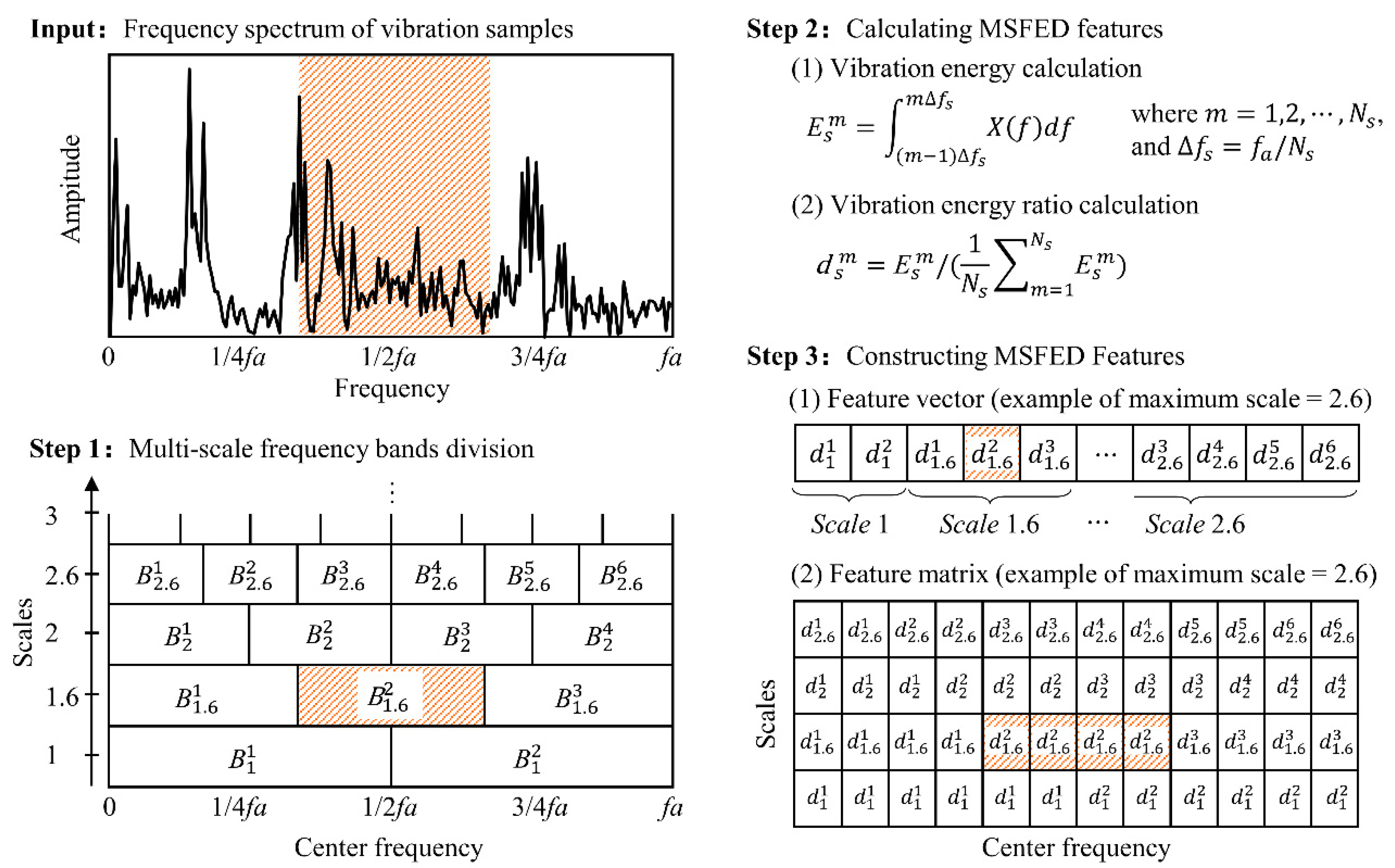
Figure 1. Scheme of the construction of the MSFED feature.
Machines 10 00743 g001
Figure 2. The two-class dataset and their ICD and BCD set distribution: (ac) the data plot, the histograms of distances and empirical cumulative distribution functions of low separability dataset, (df) the data plot, the histograms of distances and empirical cumulative distribution functions of high separability dataset.
Machines 10 00743 g002
Figure 3. Experiment setup: (a) the gearbox testing rig, (b) artificial damages (arrows were used to point out the position of damages).
Machines 10 00743 g003
Figure 4. The MSFED-1 feature vectors and MSFED-2 feature maps of vibration samples at 1000 rpm: (af), The MSFED-1 features of NC, G2, G4, OF, IF, and BF samples, (gl), The MSFED-2 features of NC, G2, G4, OF, IF and BF samples.
Machines 10 00743 g004
Figure 5. Diagnostic accuracy of different features and models on four tasks: (a) T1, (b) T2, (c) T3, and (d) T4.
Machines 10 00743 g005
Figure 6. The CWRU bearing testing rig: the motor (left), the torque sensor/encoder (middle) and the dynamometer (right).
Machines 10 00743 g006
Figure 7. The MSFED-1 and MSFED-2 features of vibration samples at 1 hp: (ad) MSFED-1 features of NC, OF7, IF7, and BF7 samples, (eh) MSFED-2 features of NC, OF7, IF7, and BF7 samples.
Machines 10 00743 g007
Figure 8. Diagnostic accuracy of different features and models on four tasks: (a) T1, (b) T2, (c) T3, and (d) T4.
Machines 10 00743 g008
Table 1. Description of the gearbox dataset.
Rotating Speed (rpm)Fault TypesNumber of SamplesClass Label
800 & 1000 & 1200NC50 & 50 & 500
800 & 1000 & 1200G250 & 50 & 501
800 & 1000 & 1200G450 & 50 & 502
800 & 1000 & 1200OF50 & 50 & 503
800 & 1000 & 1200IF50 & 50 & 504
800 & 1000 & 1200BF50 & 50 & 505
Table 2. The parameter value used in features construction.
FeaturesParametersSize
StatisticalMax, Min, Mean, Peak to peak, ARV, Var, Std, Kurtosis, Skewness, rms, Form factor, Crest factor, Impulse factor, Clearance factor1 × 14
FFT spectrumnone1 × 4800
STFTAnalytic frequency range: 0~12,000 Hz, window length: 0.002 s, Overlap rate: 0.564 × 64
OFSCohAnalytic frequency range: 0~12,000 Hz, analytic cyclic order: 0~1064 × 64
MSFED-1Analytic frequency range: 0~12,000 Hz, scales: 1~61 × 219
MSFED-2Analytic frequency range: 0~12,000 Hz, scales: 1~664 × 64
Table 3. Dataset information of four fault diagnosis tasks.
TasksSNRTraining DataTesting Data
Rotating Speed (rpm)Number of SamplesRotating Speed (rpm)Number of Samples
T1No noise800 & 1000 & 12005 × 6 × 3800 & 1000 & 120045 × 6 × 3
T2No noise800 & 1000 & 1200(25 & 15 & 15 & 5 & 5 & 5) × 3800 & 1000 & 120025 × 6 × 3
T3No noise100050 × 6 × 1800 & 120050 × 6 × 2
T40 dB800 & 1000 & 120025 × 6 × 3800 & 1000 & 120025 × 6 × 3
Table 4. Hyperparameter settings of the ten models.
ModelsFixed ParametersTunable ParametersNumber of HSs
Softmax//1
KNN
Nearest neighbor search method: the exhaustive search algorithm
Standardize the features: True
The number of neighbors: 1, 5, 10, 15
The distance metrics 1: Cosine, Euclidean, Mahalanobis 2
12
SVM
Coding design: one-vs-one
Optimization routine: the Iterative Single Data Algorithm
The box constraint: 0.01, 0.1, 1.0, 10, 100
The kernel function: gaussian, linear, polynomial3
The kernel scale: 0.01, 1.0, 100
Standardize the features: True, False
90
LDA
The discriminant type: Linear
The Linear coefficient threshold: 0
The Amount of regularization: 0, 0.2, 0.5, and 1.0
4
NB/
The data distributions: Kernel density estimation, the Multinomial distribution, the Multivariate multinomial distribution, and the normal distribution
Kernel type: box, epanechnikov, normal, triangle
16
RF
Tree: the standard CART
Number of trees: 100
The maximal number of decision splits: 5, 10, 40
The minimum number of leaf node observations: 5, 10, 40
The number of features to select at random for each split: 5, 10, 40
The split criterion: the Gini’s diversity index, the maximum deviance reduction
54
ANN
Structure: FC×2-Softmax
Training Solver: the LBFGS
Sizes of the fully connected layers: 50-10, and 50-25
The activation functions: ReLu, Sigmoid
The L2 regularization term strength: 0.001, 0.01, 0.1, 1.0
Standardize the features: True, False
32
Chen CNN
Structure: (Conv-GN-Pooling-ReLu)×2-(FC-GN-Dropout)×2-Softmax
Convolution kernel size: 3 × 3
Size of the FC layers: 120-84, and 60-42
Size of GN: 4, 8, 16
Dropout rate: 0.2, 0.5
12
Yang CNN
Structure: (Conv -Pooling-BN-ReLu-Dropout)×3-FC-Softmax
Convolution kernel size: 3 × 3
Pooling kernel size: 2 × 2
The number of kernels in convolutional blocks: 4-8-16, and 8-16-32
Size of the FC layer: 100, 200
Dropout rate: 0.2, 0.5
8
Islam CNN
Structure: (Conv-Pooling-ReLu)×3-FC-Softmax
Convolution kernel size: 3 × 3
Pooling kernel size: 2 × 2
The number of kernels in convolutional blocks: 64-64-64, 32-32-32
Size of the FC layer: 1024, 512, 256
6
1 The text in regular style is the parameter names, and the text in italic style is the parameter settings. 2 Number of HSs = Number of hyperparameters settings.
Table 5. The average accuracy of the top-three accuracies.
FeaturesAverage Accuracy of Top 3 (%)
T1T2T3T4
Statistical67.0074.9041.1074.33
FFT spectrum100.00100.0086.89100.00
MSFED-1100.00100.00100.00100.00
OFSCoh97.4095.4297.7295.78
STFT98.8499.5189.8398.62
MSFED-2100.00100.00100.00100.00
Table 6. The DSIs of six initial features on the gearbox dataset and the bearing dataset.
FeaturesDSIsDTIs
800 rpm1000 rpm1200 rpmAverage1000→800 rpm1000→1200 rpmAverage
SI0.450.430.440.4401.370.921.145
FFT spectrum0.700.690.710.7000.890.960.925
MSFED-10.680.700.710.6971.120.870.995
OFSCoh0.490.440.450.4602.571.772.170
STFT0.420.470.440.4431.702.101.900
MSFED-20.660.690.720.6901.120.901.010
Table 7. Description of the CWRU bearing dataset.
Load (hp)Fault TypesSeverity (mils)Number of SamplesLabel
0 & 1 & 2 & 3NC/50 & 50 & 50 & 500
0 & 1 & 2 & 3OF750 & 50 & 50 & 501
0 & 1 & 2 & 3OF1450 & 50 & 50 & 502
0 & 1 & 2 & 3OF2150 & 50 & 50 & 503
0 & 1 & 2 & 3IF750 & 50 & 50 & 504
0 & 1 & 2 & 3IF1450 & 50 & 50 & 505
0 & 1 & 2 & 3IF2150 & 50 & 50 & 506
0 & 1 & 2 & 3BF750 & 50 & 50 & 507
0 & 1 & 2 & 3BF1450 & 50 & 50 & 508
0 & 1 & 2 & 3BF2150 & 50 & 50 & 509
Table 8. Dataset information of four fault diagnosis tasks.
TasksSNRTraining DataTesting Data
Load (hp)Number of SamplesLoad (hp)Number of Samples
T1No noise0 & 1 & 2 & 35 × 10 × 40 & 1 & 2 & 345 × 10 × 4
T2No noise0 & 1 & 2 & 3(25 & 15 & 15 & 15 & 10 & 10 & 10 & 5 & 5 & 5) × 40 & 1 & 2 & 325 × 10 × 4
T3No noise050 × 10 × 11 & 2 & 350 × 10 × 3
T40 dB0 & 1 & 2 & 325 × 10 × 40 & 1 & 2 & 325 × 10 × 4
Table 9. The average accuracy of the top-three models.
FeaturesAverage Accuracy of Top 3 (%)
T1T2T3T4
Statistical94.7294.73 85.8393.16
FFT Spectrum99.8399.5060.5899.60
MSFED-199.9999.9194.1499.41
OFSCoh99.1499.1097.8796.16
STFT97.3597.3392.1794.31
MSFED-299.9199.9594.2499.36
Table 10. The DTIs of six features on the gearbox dataset and the bearing dataset.
FeaturesDSIsDTIs
0 hp1 hp2 hp3 hpAverage0→1 hp0→2 hp0→3 hpAverage
SI0.490.490.510.470.4906.674.773.214.883
FFT spectrum0.670.670.680.690.6780.830.860.800.830
MSFED-10.620.640.650.650.6401.030.930.790.917
OFSCoh0.510.530.540.550.5331.461.341.171.323
STFT0.440.440.460.450.4483.783.332.433.180
MSFED-20.620.630.650.650.6381.210.990.871.023
Publisher’s Note: MDPI stays neutral with regard to jurisdictional claims in published maps and institutional affiliations.