Abstract
The manufacture, maintenance and inspection of a ship involve a series of works on the ship shell plate, which were always seen as harmful for human operators and time-consuming work. The shipping industry is looking to replace manual work with automation equipment. A magnetic climbing robot that can omnidirectionally move on ship shell plate was presented in this paper. This article summarized the mechanical structure, control system, kinematic model, and autonomy of robot. The mechanical structure of the robot was inspired by bionics and adopted a wheel-leg hybrid locomotion system. In the control system of this robot, industrial control computer (IPC) was adopted as the core controller and brushless direct current servomotor was chosen as the actuating station. Finally, the motion analysis of the designed robot was performed. The results of the analysis show that the magnetic climbing robot adapted to the ship curved shell plate and crossed obstacles.
1. Introduction
Under the background of economic globalization, the shipping industry has been developing rapidly. The manufacture, maintenance, inspection and other operations of large ships, due to the large, curved shape, long length and complex operating environment, are mostly completed by manual operations. Manual operations have disadvantages, such as high cost and low efficiency, and the trend of applying automation equipment to replace manual operations is becoming stronger and stronger. Therefore, the design of magnetic climbing robots that can replace manual work is very important in the shipping industry.
To solve the problem how the magnetic climbing robot adsorbs on the ship shell plate, researchers have completed a lot of research [1,2,3,4,5,6,7,8]. Generally speaking, the metal materials used in the ship shell plate are all magnetically conductive materials, the non-contact magnetic adsorption scheme has two characteristics of strong adsorption capacity and low movement resistance, which can make the robot move smoothly on the ship shell plate. This scheme is the most valuable option.
Wheeled locomotion, tracked locomotion and legged locomotion are the three common locomotion methods of magnetic climbing robots. When the magnetic climbing robot is moving on a smooth ship shell plate, the wheels can simply and effectively achieve high-speed and energy-efficient locomotion. However, when there are obstacles on the ship shell plate, wheeled locomotion cannot safely and smoothly cross. The tracked locomotion has a certain ability to overcome obstacles, the contact surface with the wall is much larger than that of the wheeled locomotion. They usually move slower and with lower energy efficiency. In addition, they cannot move on ship curved shell plate.
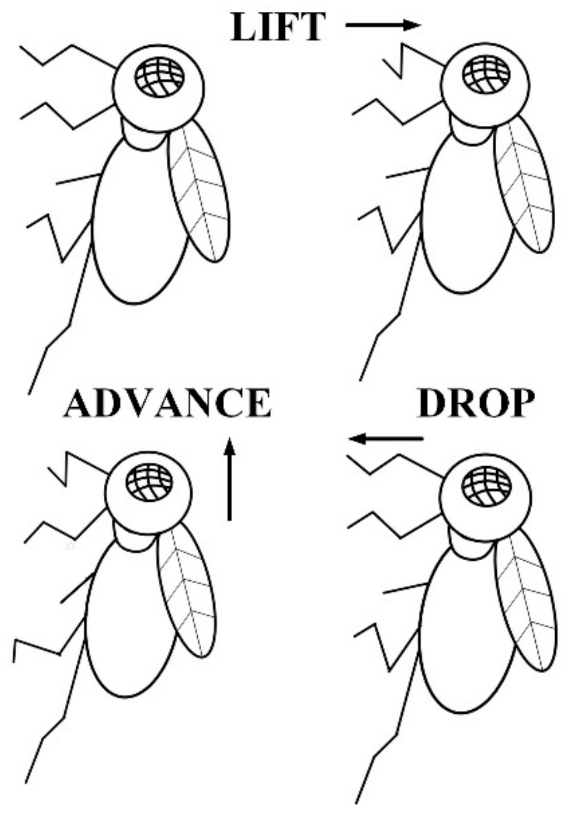
Unlike wheeled locomotion and tracked locomotion, legged locomotion is biologically inspired. Legged locomotion is the most effective solution when dealing with complex wall environments and obstacles. However, legged locomotion also has the disadvantage that it moves slower and with lower energy efficiency. In addition, legged locomotion is expensive and complex to control. To overcome the disadvantages of legged locomotion, its complex structure should be simplified, by observing the locomotion of flies, as shown in Figure 1. It was found that the legged locomotion can be divided into three actions: lifting, advancing, and dropping the leg. The advancing action can be replaced by wheel rolling, which can combine the advantages of wheeled and legged locomotion. The surface of ship shell plate is smooth and has slat barriers, and the hybrid wheel-leg design can better meet the work requirements.

Figure 1.
Locomotion of flies.
At present, the research of wheel-legged hybrid magnetic climbing robot is still relatively scarce. However, there has been a lot of reference research on wheel-leg hybrid robots applied to ground locomotion. Nagano et al. designed a wheel-leg hybrid robot that has four legs, each with two shock-absorbing devices and two joints, and feet with wheels [9]. Although the robot can adapt to many types of rough and uneven ground, when the application environment was changed to the ship shell plate, the installation and stability of the adsorption device became a problem. Li et al. designed a six wheel-legged robot [10]. The six legs were evenly distributed around the circular platform on which they support. If the robot was applied to ship shell plate, adsorption device can be added to its abdomen position, and the robot can also remain stable when one leg was lifted. The motion control of this kind of robot is more complicated.
The above studies showed that the six-wheeled-legged hybrid robot was more stable than the four-wheeled-legged hybrid robot during motion. Motion stability was an important requirement for designing magnetic climbing robots. The six wheeled-legged hybrid robot was designed by Ernesto Christian Orozco-Magdaleno. It has three legs installed on the left and right sides, each leg has joints and the wheels are installed on the feet [11]. If the robot is installed on a suction device and works on the ship shell plate, the flexion of the joints can affect its load capacity. Replacing the bending function with the lifting function can better adapt to the environment of the ship shell plate. In this paper, a six wheel-legged hybrid robot applied to ship shell plate was proposed. The mechanical structure and working principle of the magnetic climbing robot were explained. The control system of the magnetic climbing robot was introduced. The kinematics model of the magnetic climbing robot was established and analyzed. The path tracking approach of the magnetic climbing robot was described. Finally, the motion of the magnetic climbing robot was simulated and analyzed.
2. Design of Mechanical Structure and Control System
2.1. Mechanical Structure and Working Principle
The starting point of the mechanical structure design of the magnetic climbing robot is the goal of combining the advantages of wheeled locomotion and legged locomotion. We were inspired by observing the locomotion of flies, as discussed in the previous section. Then combined some examples of wheel-legged hybrid robots working on the ground, drawing on the advantages of different designs. We propose a reasonable and efficient mechanical structure of a magnetic climbing robot, as shown in Figure 2. The mechanical structure was composed of the following designs:
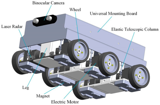
Figure 2.
Mechanical structure of magnetic climbing robot.
- (1)
- Three legs that can complete telescopic motion were installed in the middle of the abdomen of robot.
- (2)
- A wheel was installed on each side of the foot position of each leg, and the wheel was driven by brushless DC servomotor on the inside.
- (3)
- The magnet was installed under the brushless DC servomotor, which can move up and down with the lifting and dropping of the leg to achieve the adjustment of the magnetic force.
- (4)
- Elastic telescopic columns connect the wheels to the robot body, and they allow the magnetic climbing robot to cope with the curvature of ship shell plate.
- (5)
- The universal mounting board was supported on the top of the magnetic climbing robot by small columns.
The motor driver and the lower computer were placed inside the magnetic climbing robot. The laser radar was on the front of the magnetic climbing robot. The binocular camera was installed at the front of the universal mounting board. Additional sensors were placed inside the robot as required by the work. The working principle of this mechanical structure was the following:
- (1)
- The magnet keeps a distance from ship shell plate, which can not only reduce the resistance during work but also make the magnetic climbing robot easy to adapt to the curved surface.
- (2)
- The wheel speed of each wheel can be controlled individually, and the direction of the magnetic climbing robot can be controlled by adjusting the speed difference between the wheels on both sides.
- (3)
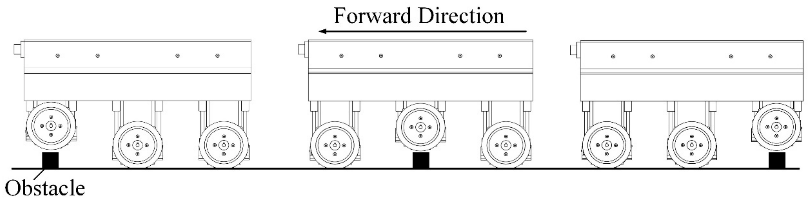
- When the laser radar detects that there was an obstacle in front of the robot, the first leg, the second leg and the third leg of the robot will be lifted in turn. After crossing the obstacle, the three legs will drop in turn, so that the robot can cross the obstacle as a whole, as shown in Figure 3.
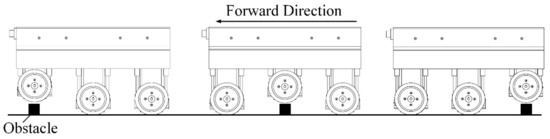 Figure 3. Over obstacles.
 - (4)
- The leg and wheel of the magnetic climbing robot were not in direct contact, but they were connected to the splint above. When ship shell plate has curvature, the wheel can adapt to the curved surface due to the characteristics of the elastic telescopic column, and the elastic telescopic column can be compressed when the leg is lifted, thereby driving the wheel to rise.
- (5)
- Various work equipment can be installed on the universal mounting board to increase the function of the magnetic climbing robot.
Since the working environment of the magnetic climbing robot was on the ship shell plate, considering the safety of its work, the magnetic climbing robot did not load batteries. Each component was mounted with enough gaps to make sure there was no conflict of signal interference that creates sensor error.
2.2. Design of Control System
The control system of the magnetic climbing robot adopts a distributed system in which the industrial personal computer (IPC) controls the driving node through controller area network (CAN). This technology was relatively mature and had many research applications [12,13,14]. Compared with the general bus technology, CAN has the characteristics of high transmission rate, better error mechanism and high resistance to electromagnetic interference [15]. CAN can be configured with up to 128 nodes. In this control system, the IPC was used as the master node, and other devices were used as slave nodes.
2.2.1. Hardware Design of Control System
As shown in Figure 4, the hardware of this control system was mainly composed of IPC, USB-CAN communication module, Motor driver, STM32, etc. The computer realizes the communication on the CAN bus through USB-CAN communication module. The magnetic climbing robot had six sets of motor drivers, which need to control the operation of six brushless direct current motors at the same time and receive feedback from six encoders at the same time. STM32 was used as the lower computer to process the control information of the robot obstacle avoidance module. The obstacle avoidance module consisted of lifting motors and sensors. Lifting motor was controlled by relay. Sensors had binocular cameras and laser radar. Binocular camera was used to obtain macroscopic information of working environment. Laser radar was used for obstacle identification and distance measurement.
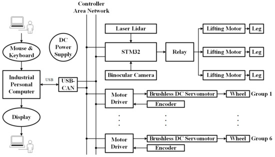
Figure 4.
Schematic diagram of the hardware structure of the control system.
2.2.2. Software Design of Control System
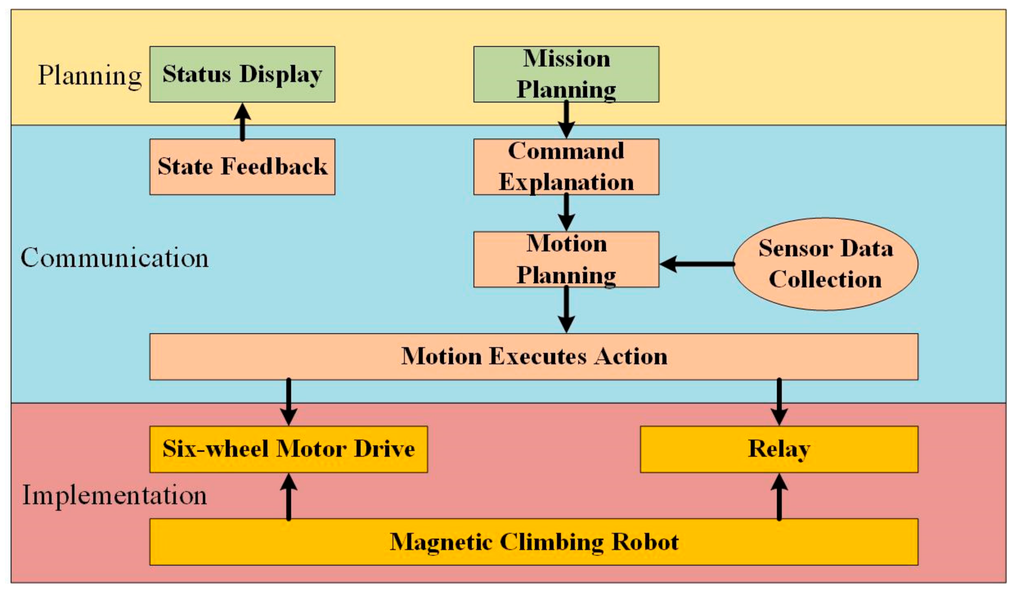
The structure of the magnetic climbing robot control software was shown in Figure 5, which was divided into three layers. The planning layer at the top was responsible for the planning of robot motion, the communication layer was responsible for communication and command interpretation and the execution layer was responsible for completing the execution operation. According to the basic motion type of the robot, it was divided into barrier-free motion module and obstacle-avoidance motion module. The planning results were sent to each actuator of the robot through USB-CAN communication module. The USB-CAN communication module “translated” the communication protocol into the tasks to be performed and controlled each actuator. The actuator included wheel mechanism and leg mechanism. The control of the leg mechanism was performed by issuing commands to the relays. The motor control program module of the wheel adopted profile velocity mode and profile position mode. According to the research in part 3 of this paper, the linear velocity and angular velocity of the robot were converted into the control quantities of six motors.
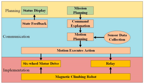
Figure 5.
Schematic diagram of robot software architecture.
3. Motion Analysis
3.1. Kinematic Analysis
The kinematic analysis of the magnetic climbing robot can be divided into two parts, the first part was to analyze the motion of the legs, and the second part was to analyze the chassis motion. Providing a theoretical basis for the motion control of magnetic climbing robots.
3.1.1. Kinematic Analysis of Leg Motion
The obstacle crossing and adsorption force adjustment of the magnetic climbing robot were realized by the motion of leg. The motion state of leg was different when dealing with different ship shell plate. Three motion states of the legs of the magnetic climbing robot were introduced when working on the ship flat shell plate, the ship curved shell plate and the ship shell plate with obstacles.
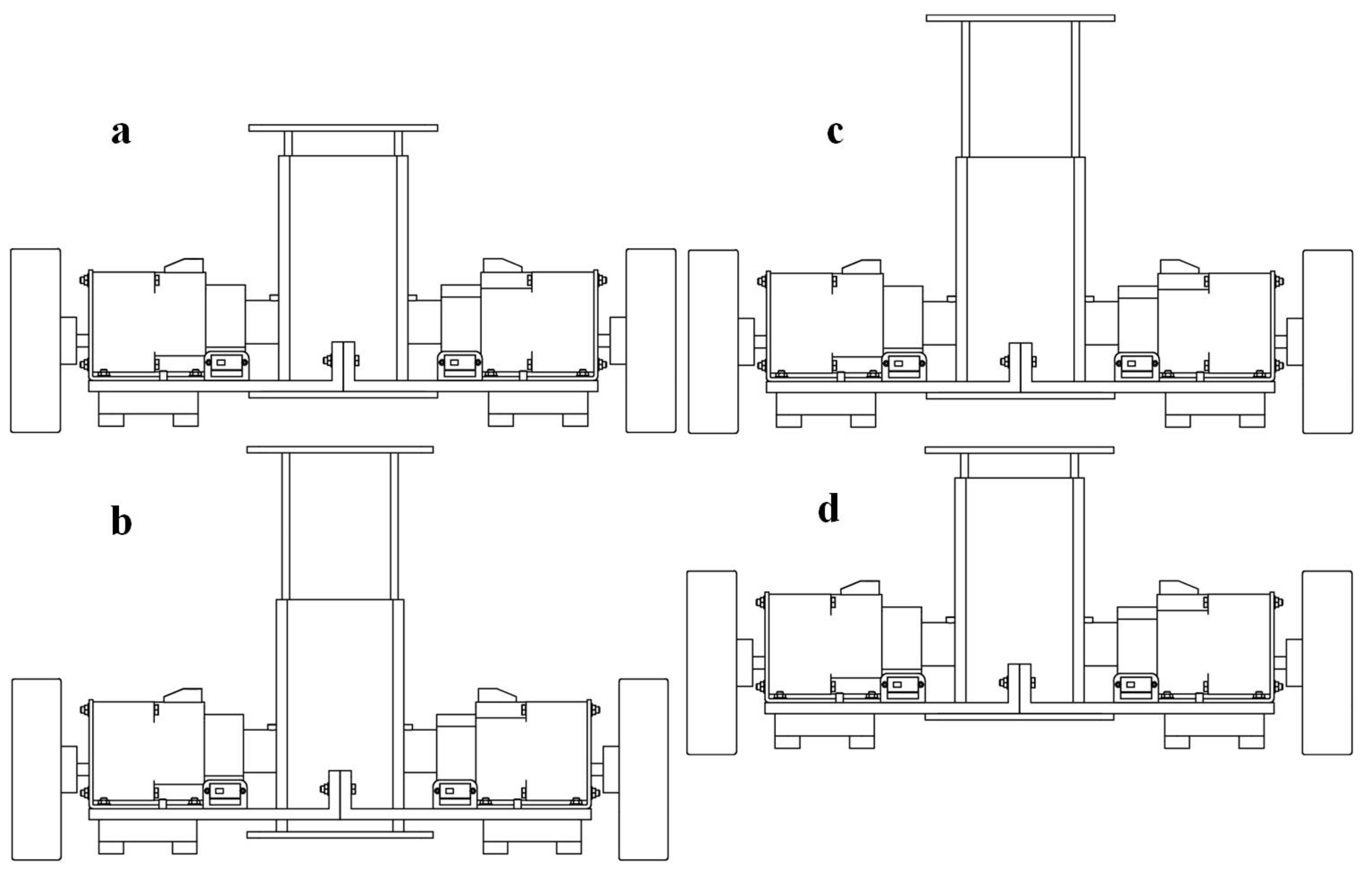
When the magnetic climbing robot worked on the ship flat shell plate, the bottoms of the six wheels of the robot were all on the same plane. It can be achieved by directly retracting the legs to the shortest length, as shown Figure 6a. At this time, the gap between the magnet and the wall was the shortest, and the height of the robot was the lowest.
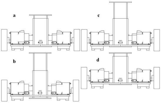
Figure 6.
Obstacle crossing state: (a) shortest length, (b) longest length, (c) contact, (d) lift.
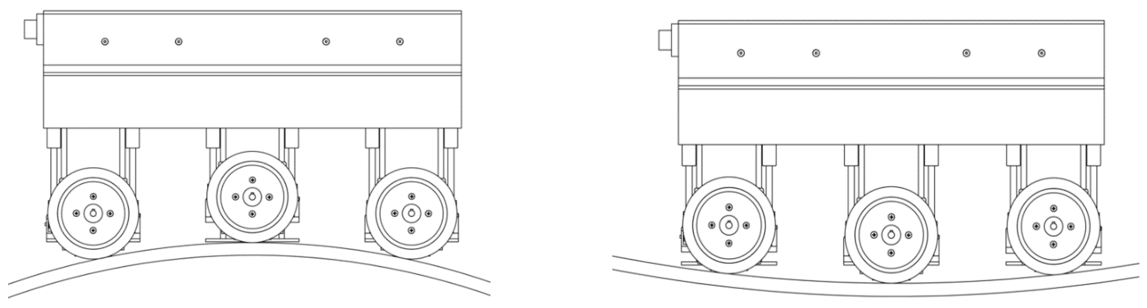
When the magnetic climbing robot worked on the ship curved shell plate, as shown in Figure 7, the bottoms of the six wheels of the robot were all on the different plane. At this time, the height of each wheel needs to be inconsistent, and it can be achieved by extending the length of the legs to the longest, as shown Figure 6b. In this state, the gap between the magnet and the wall was still the shortest, but the height of the robot was the highest.
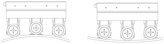
Figure 7.
Movement on the ship curved shell plate.
As previously mentioned, the magnetic climbing robot needed to lift its three legs when it was working to overcome obstacles. Assuming that the robot can lift 10 units, the magnet can lift 10 units and the legs can lift 12 units. The motion process of leg was shown in Figure 6. When the laser radar detected an obstacle, three legs were first adjusted from (a) to (b). Both (a) and (b) have been carefully introduced in the previous section. (c) represents the movement of the leg to a position where the height of the magnet can be controlled, at which time the height of the magnet remains unchanged, but the leg has risen. (d) Indicates that the leg has lifted the magnet to the highest position, and the wheel has reached a height that can cross the obstacle. After the wheel passed the obstacle, the leg moved from (d) back to (b).
The height control curve of each component during leg locomotion was shown in Figure 8.
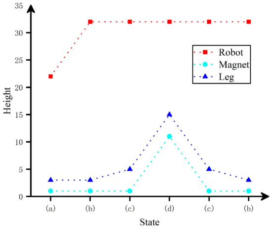
Figure 8.
Height control curve.
3.1.2. Kinematic Analysis of Chassis Motion
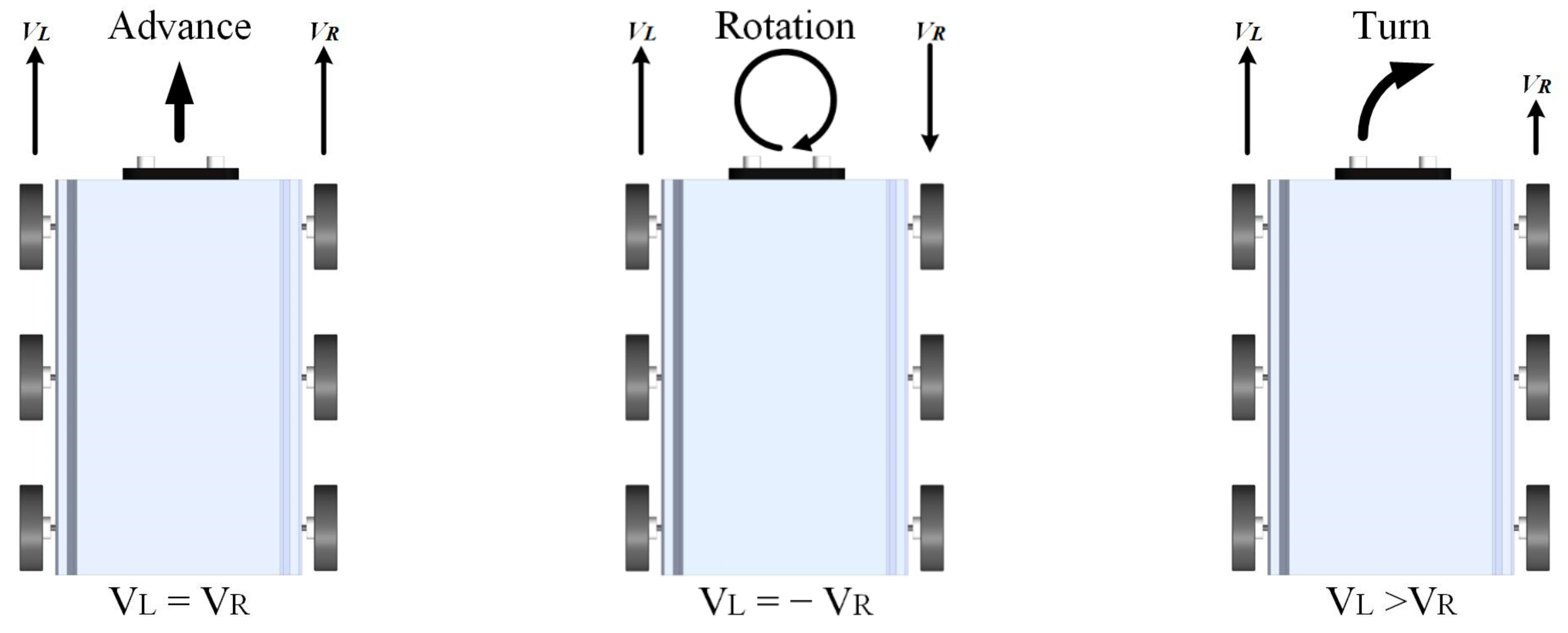
According to the literature [16,17], differential steering can be used in the design of a six-wheeled robot. The magnetic climbing robot can be moved in all directions on the ship shell plate by using the differential steering model. As depicted in Figure 9, the difference in the speed of the wheels on both sides determines the driving direction of the magnetic climbing robot.
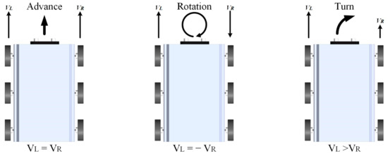
Figure 9.
The principle of differential steering.
To realize the differential steering motion of the robot, it is necessary to establish the kinematics model of the chassis to find the relationship between the pose, speed and wheel speed of robot when moving on ship shell plate. The speed of the wheels was determined by the motor brushless DC servomotor. During the actual motion, the model may differ from the ideal situation due to acceleration, deceleration or steering. To find the relationship of the chassis motion parameters, several conditions need to be assumed:
- (1)
- Six drive wheels were symmetrically distributed on the same plane.
- (2)
- The deformation of the wheel was negligible, and the contact with the ship shell plate was a point. The radius of the wheel was r.
- (3)
- The geometric center point C of the chassis coincided with the projection of the center of mass on the ship shell plate.
- (4)
- The wheels simply rolled on the ship shell plate, and there was no slippage.
- (5)
- Assuming that the ship shell plate was a rigid body, the deformation of the ship shell plate was ignored.
- (6)
- Longitudinal slip was not considered when turning.
- (7)
- The robot was in a state of steady motion.
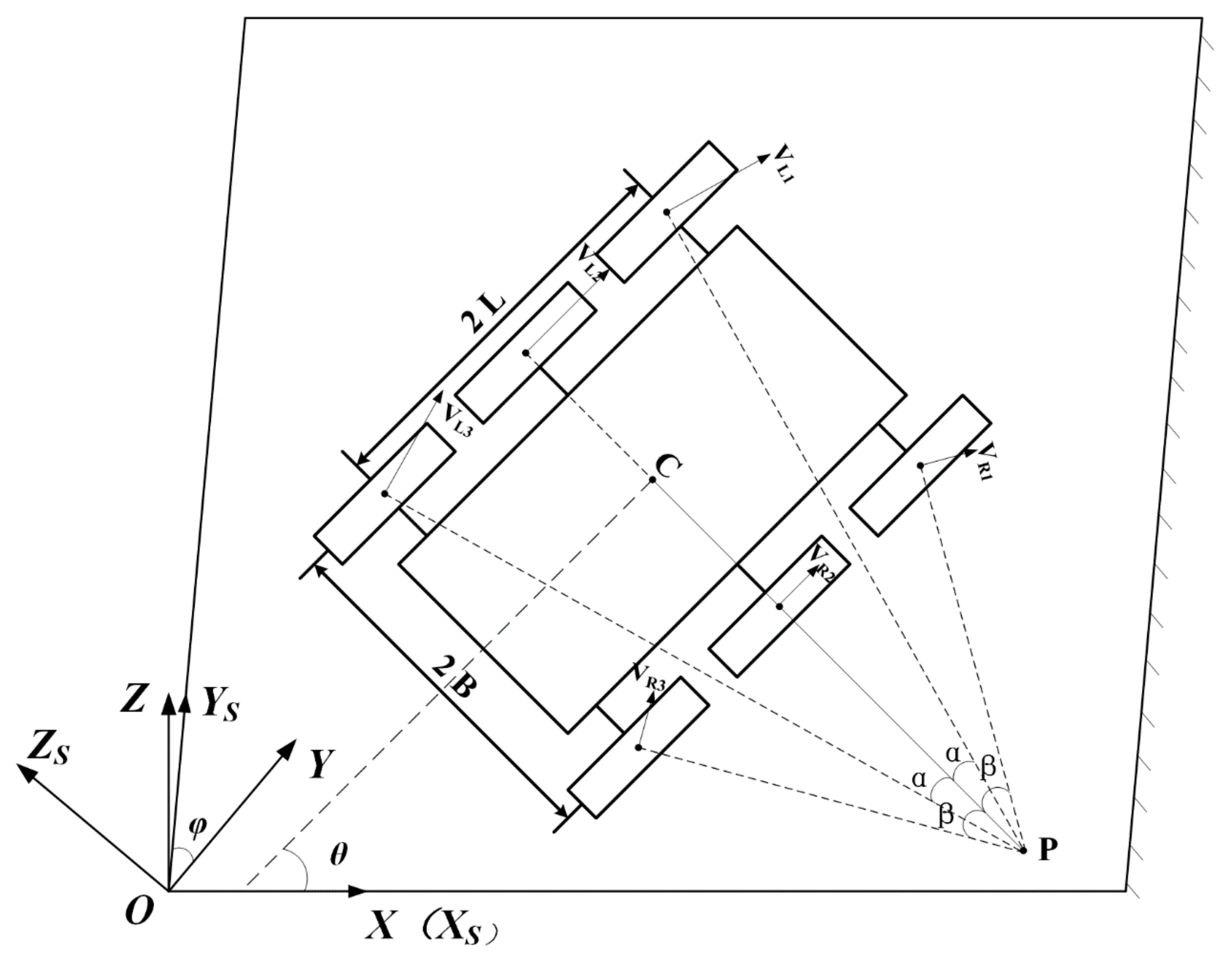
During the movement of the magnetic climbing robot. It needs to continuously acquire its pose changes, that is, its position and orientation on the plane that are constantly changing. Considering that the chassis moves on a two-dimensional plane, first establish a two-dimensional coordinate system in the world coordinate system, and mark the parameters of the chassis model, as shown in Figure 10.
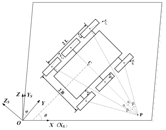
Figure 10.
Schematic diagram of chassis motion model.
Figure 10 shows the chassis motion model of the magnetic climbing robot. The symbols and model parameters in the Figure 10 were shown in Table 1.

Table 1.
Parameter symbol description table.
The actual linear velocity direction of the wheel can be decomposed into the front wheel speed Vijf and the side speed Vijs:
If the magnetic climbing robot was controlled to rotate in place, for the wheels on both sides, the speed was the same and the direction was opposite, the speed Vijf in front of the wheel was 0, and the speed in the side direction was . At this time, the instantaneous rotation center point P of the chassis was located at the geometric center point C, and the chassis was in a circular motion with C as the center and L as the radius.
The relationship between the angular velocity of the chassis and the linear velocity of the left and right wheels was as follows:
When the magnetic climbing robot performs a steering motion, the wheels on both sides have different speeds and the same direction. When the speed of the left wheel was greater than that of the right, the robot turns to the right, and when the speed of the right wheel was greater than the left, the robot turns to the left.
The relationship between the motion of the geometric center point C of the chassis and the linear speed of the driving wheels on both sides defined as:
Establish the kinematics model of the chassis geometric center point C:
The relationship between the steering angular velocity ω and the steering radius R of the chassis and the linear velocity of the left and right wheels was expressed as:
Combine the two formulas to get:
When the magnetic climbing robot moves forward, that is, when X tends to infinity the wheels on both sides have the same speed and the same direction, and the linear speed of the wheels is the forward speed of the robot.
According to the above analysis, the kinematic laws of pose and velocity changes were obtained. It provided a theoretical basis for the path tracking of the magnetic climbing robot.
3.2. Path Tracking
Path tracking is one of the key problems of motion control for magnetic climbing robots, which is denoted as tracking a predetermined path by controlling the lateral and yaw movement of the vehicle [18]. Thus, it can be defined as minimizing the lateral offset and heading errors [19]. The predetermined path of the magnetic climbing robot when working on the outer panel of the ship is generally planned in advance according to the work needs.
Academia had proposed many different path tracking methods in the past many years, which could be mainly divided into two types: based on classical control theory and based on geometric solution. This paper was based on pure pursuit algorithm, a typical representative of the latter, which was widely used in low-speed scenarios. The working scene of the magnetic climbing robot on the ship shell plate was a low-speed scene.
Figure 11 explains the principle of pure pursuit. In the robot coordinate system, the robot obtained a target point on the reference path through the look-ahead distance l. Then, the robot reached the target point through an arc trajectory. The turning radius was r. Δx was the horizontal distance of O to the target point. We set the coordinates of the target point to be (x,y).
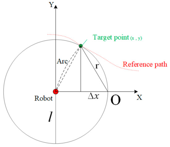
Figure 11.
The principle of pure pursuit.
Formulas (9)–(11) can be obtained from the geometric relationships in Figure 11. Simultaneous formulas obtain the relationship between look-ahead distance and turning radius.
The process of pure pursuit can be summarized by the following steps:
- (1)
- Defined the initial position of the robot in the wall coordinate system.
- (2)
- Calculated the Euclidean distance between all points on the reference path and the robot and took the point with the smallest Euclidean distance.
- (3)
- Determined the look-ahead distance l, start from the point with the smallest Euclidean distance and look for the target point with a distance l from the robot in the forward direction of the path.
- (4)
- The position of the target point in the wall coordinate system was transformed into the robot coordinate system.
- (5)
- The turning radius r was calculated according to Formula (12).
- (6)
- The turning radius was calculated as the linear speed of the wheels on both sides, and the position of the robot was continuously updated.
- (7)
- The robot chased the advancing target point and keep driving on the predetermined path.
From Formula (12), the key to path tracking was to determine the look-ahead distance l. The traditional pure pursuit algorithm set a fixed look-ahead distance l according to the working environment in real use. However, there were also some problems with this.
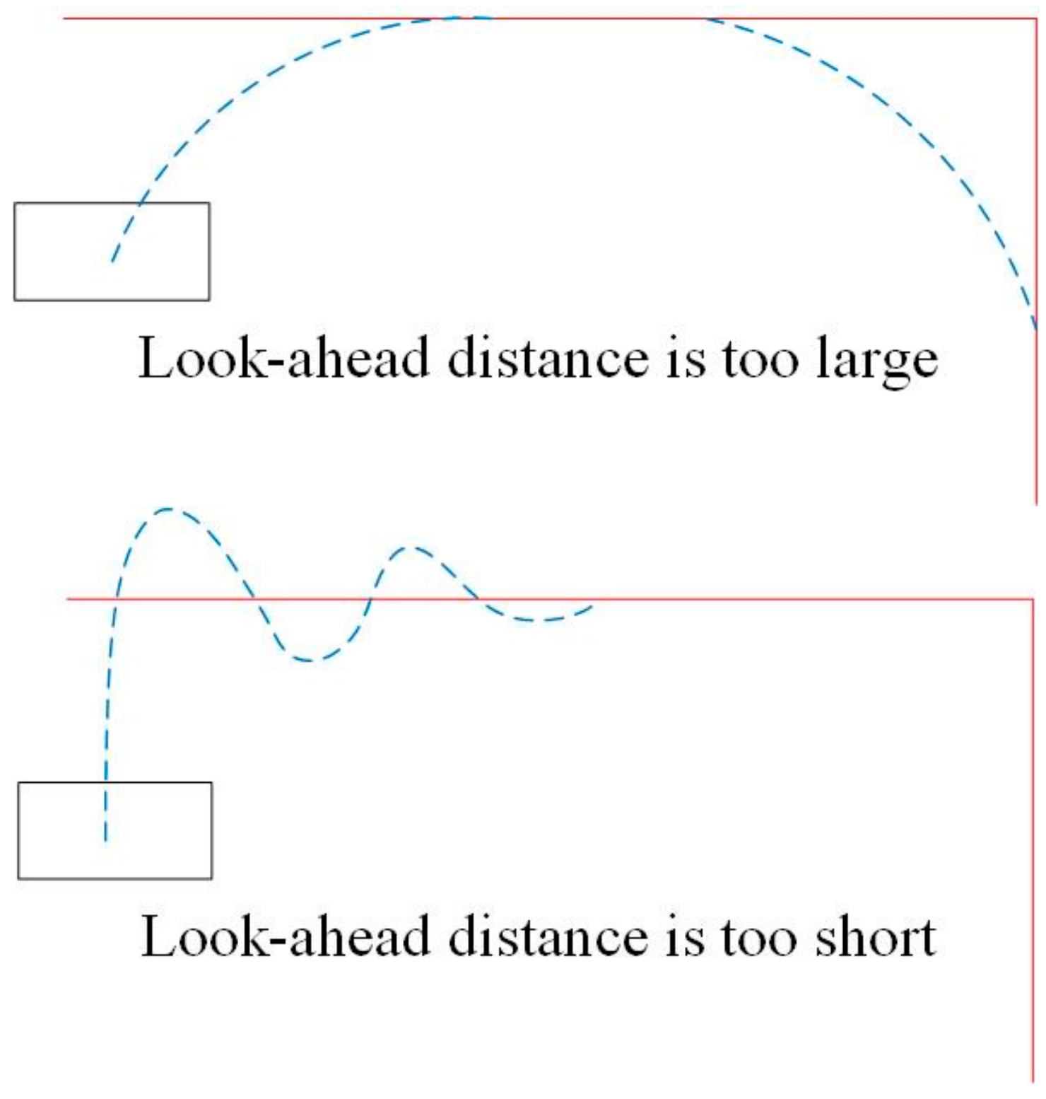
As shown in Figure 12, too large a look-ahead distance caused the robot to ignore the local path, while too short a look-ahead distance caused the robot to oscillate on the path. For the choice of recommended look-ahead distance, Kuwata et al. provided that speed was one of the key factors affecting look-ahead distance [20]. They proposed a linear model that was able to derive a recommended look-ahead distance based on the current speed of robot. As shown in Formula (13):
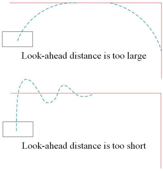
Figure 12.
The problems of pure pursuit when look-ahead distance is too large or too small.
Recommended look-ahead distances do not represent reasonableness. For the choice of look-ahead distance, there are two goals to be achieved: fit the track and run smoothly. If these two goals conflict, try to satisfy the second goal. For safety reasons, it is necessary to prevent the robot from rolling over. Figure 13 is a schematic diagram of an imminent rollover of the robot. Adding a new constraint rlimit, the magnetic climbing robot cannot operate on a path with a turning radius exceeding rlimit under any circumstances. Formula (14) is the moment equation when a rollover is imminent. Combined with the centripetal force formula, the value of rlimit can be calculated, as shown in Formula (15).
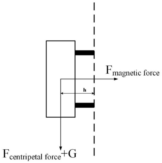
Figure 13.
The robot is about to overturn.
The recommended look-ahead distance was obtained by Formula (13), and then rrecommend was obtained by lrecommend. If rrecommend ≥ rlimit, it meant that lrecommend was reasonable and the robot can pass smoothly.
3.3. Simulation and Analysis
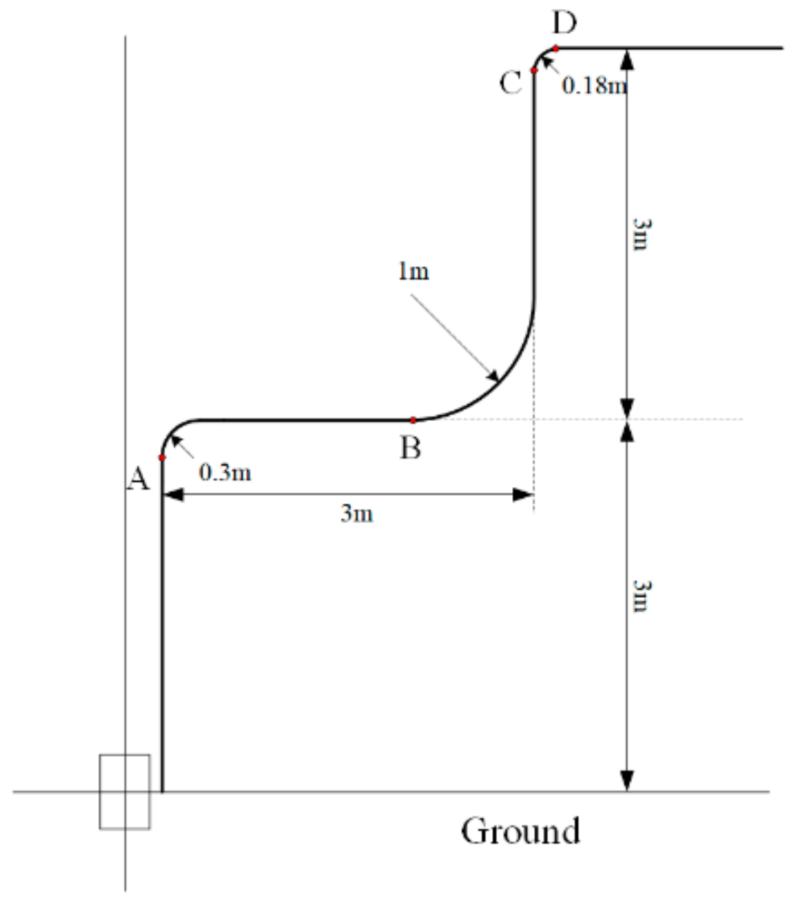
In order to verify the correctness of the kinematic model and path tracking method proposed above, simulation analysis was carried out in this section. A reference path was designed to simulate the robot moving upward from the bottom of the ship. This reference path consists of three arc paths and four straight paths, as shown in Figure 14, points A, B, and C were the initial points of the three arcs, point D was the end of the third arc.
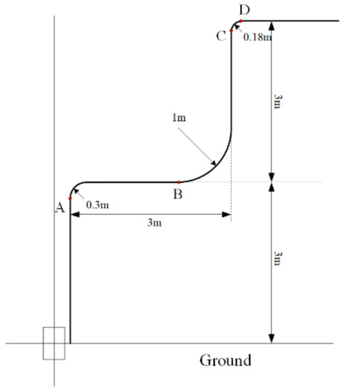
Figure 14.
Reference path.
The three arcs the robot passes through the reference path correspond to three different situations. When the robot travelled on the reference path, it passed through three arcs. When the robot passed through the first arc, the arc radius was between rrecommend and rlimit. When the robot passed the second arc, the arc radius was longer than rrecommend. When the robot passed the arc of the third segment, the arc radius was shorter than rlimit. The simulation parameter conditions that meet the appeal requirements were set as follows, as shown in Table 2.
Table 2.
Simulation parameters.
When the robot was driving on an arc, due to the kinematics model mentioned above, the wheels on both sides need different speeds to turn the robot. For example, when the robot passed the second arc of the reference path with the parameters in Table 2, the required speeds of the wheels on both sides can be obtained according to Formulas (6) and (7), , .
The linear model of look-ahead distance l and velocity is shown in Formula (16). The rrecommend is shown in Formula (17). The rlimit is shown in Formula (18).
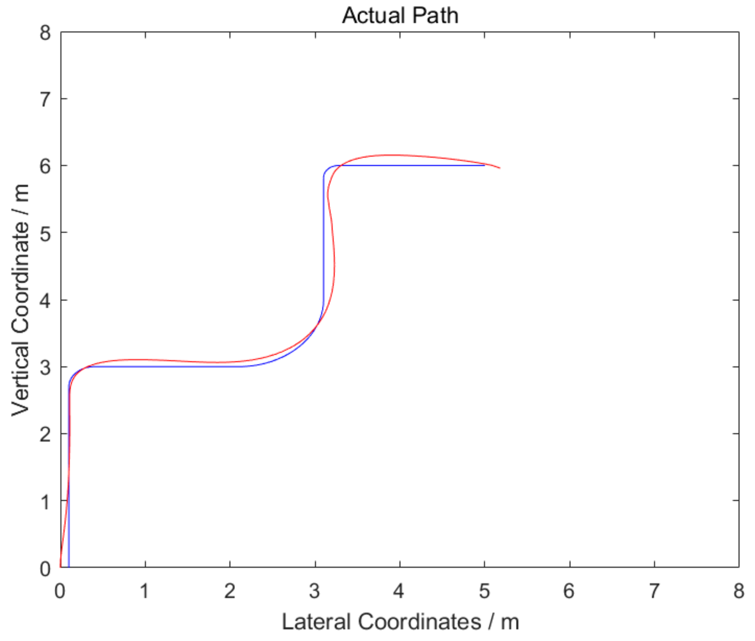
The simulation results are shown in Figure 15 and Figure 16. Figure 15 was the distribution diagram of target points, and Figure 16 was the actual travel path of the robot. The state of the robot at each position of the path was analyzed through these two figures.
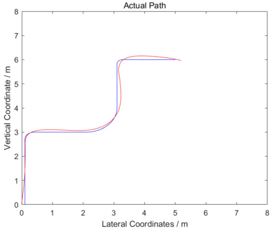
Figure 15.
Actual path.
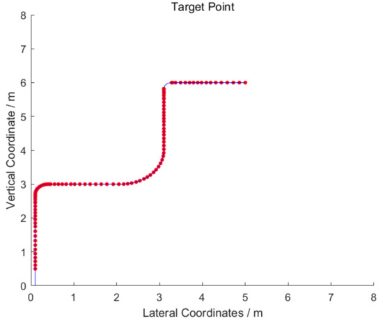
Figure 16.
Distribution map of target points.
The initial speed of the robot was 0.5 m/s, and it accelerated to 1 m/s on the first straight line path. According to Formula (16), look-ahead distance l increased from 0.5 m to 1 m. When the target point reached point A, the arc radius was between rrecommend and rlimit, the robot can pass smoothly. However, a longer look-ahead distance l can lead to a larger deviation. Therefore, the speed was reduced to 0.3 m/s, and look-ahead distance l was also reduced to 0.3 m. When the target point reached point B, the arc radius was greater than rrecommend, the robot can pass smoothly and the deviation cannot be too large, so it can pass without deceleration. When the target point reached point C, the arc radius was less than rlimit, and the robot was in danger of rolling over and cannot pass smoothly. Therefore, the target point was adjusted to point D at the end of the arc, and the speed was reduced to 0.3 m/s. Although this can cause a large deviation, smooth passage was the first consideration, and the resulting deviation can be accepted.
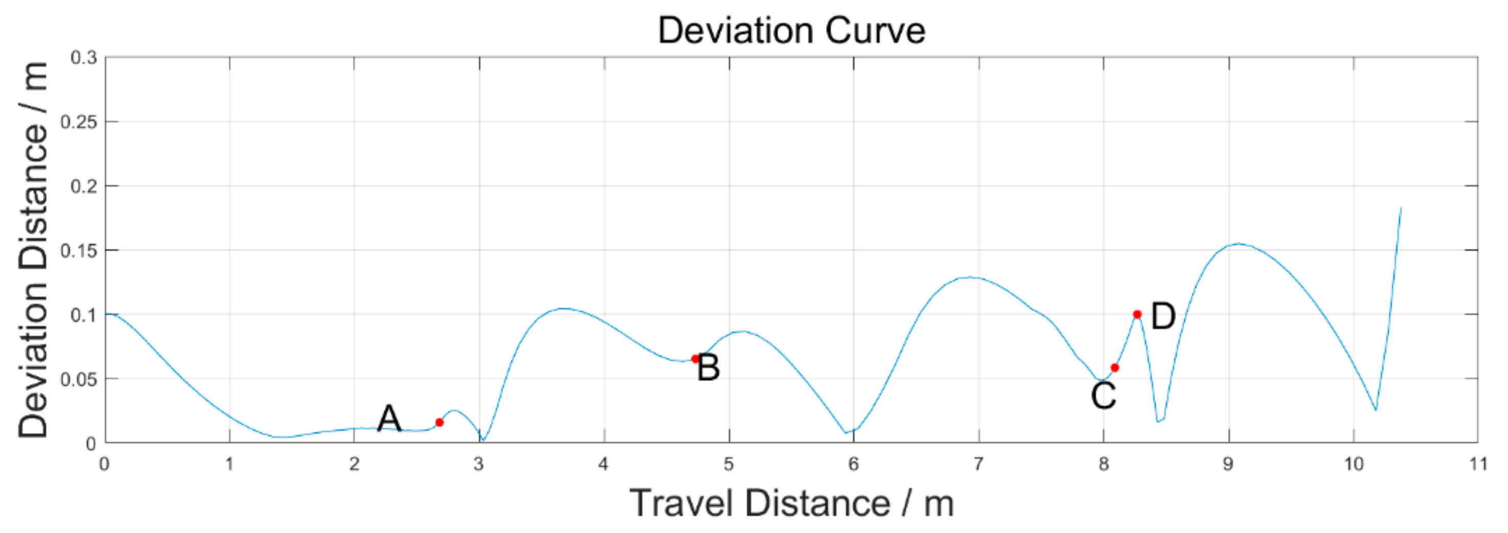
Figure 17 shows the distance deviation between the reference path and the actual path when the robot was traveling. From the figure, it can be seen that the deviation distance of the robot was controlled at about 0.1 m, from which it can be concluded that the path tracking proposed in this paper can keep the deviation distance at a low level under the premise that the robot can maintain stability. The reference path proposed in the simulation in this paper had extreme conditions. In the actual operation of the robot, the robot was prevented from passing through small arcs, thereby further reducing the distance deviation of the actual path of the robot.
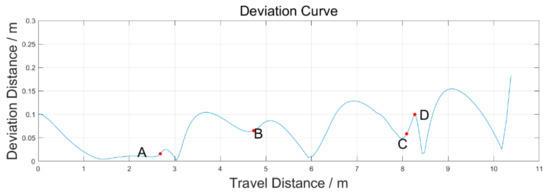
Figure 17.
Deviation distance between the actual path and the reference path.
4. Conclusions
Based on the concept of bionics and wheel-leg hybrid robots applied to ground locomotion design, a magnetic climbing robot was designed. The mechanical structure of the magnetic climbing robot and the working principle of the wheel-leg hybrid motion were briefly described. The distributed control network of the robot CAN bus communication was designed. The kinematic model of the magnetic climbing robot was studied, and its path tracking method was introduced. The simulation and analysis results show that the magnetic climbing robot can travel on the ship shell plate according to the reference path.
Author Contributions
Conceptualization, S.C. and X.P.; methodology, X.P.; software, X.P.; validation, X.P.; formal analysis, X.P.; investigation, H.S.; resources, S.C.; data curation, X.P.; writing—original draft preparation, X.P.; writing—review and editing, S.C.; visualization, P.D.; supervision, Shuwan Cui; project administration, S.C.; funding acquisition, S.C. All authors have read and agreed to the published version of the manuscript.
Funding
This research was funded by [China Postdoctoral Science Foundation] grant number [2021MD703809] and [Science and Technology Base and Talent Special Project of Guangxi Province] grant number [AD19245150] and [Guangxi University of Science and Technology Doctoral Fund] grant number [19Z27] and [Innovation Project of Guangxi Graduate Education] grant number [YCSW2022435]. And The APC was funded by [Guangxi University of Science and Technology Doctoral Fund].
Institutional Review Board Statement
Not applicable.
Informed Consent Statement
Not applicable.
Data Availability Statement
Not applicable.
Acknowledgments
All individuals agree to acknowledge.
Conflicts of Interest
The authors declare no conflict of interest.
References
- Feng, X.; Tian, W.; Wei, R.; Pan, B.; Chen, Y.; Chen, S. Application of a Wall-Climbing, Welding Robot in Ship Automatic Welding. J. Coast. Res. 2020, 106, 609–613. [Google Scholar] [CrossRef]
- Abdulkader, R.E.; Veerajagadheswar, P.; Lin, N.H.; Kumaran, S.; Vishaal, S.R.; Mohan, R.E. Sparrow: A Magnetic Climbing Robot for Autonomous Thickness Measurement in Ship Hull Maintenance. J. Mar. Sci. Eng. 2020, 8, 469. [Google Scholar] [CrossRef]
- Alkalla, M.G.; Fanni, M.A.; Mohamed, A.M.; Hashimoto, S. Tele-operated propeller-type climbing robot for inspection of petrochemical vessels. Ind. Robot 2017, 44, 166–177. [Google Scholar] [CrossRef]
- Huang, H.; Li, D.; Xue, Z.; Chen, X.; Liu, S.; Leng, J.; Wei, Y. Design and performance analysis of a tracked wall-climbing robot for ship inspection in shipbuilding. Ocean Eng. 2017, 131, 224–230. [Google Scholar] [CrossRef]
- Ravindra, S.B.; Pushparaj, M.P.; Saroj, K.P. Experimental investigations on permanent magnet based wheel mechanism for safe navigation of climbing robot. Procedia Comput. Sci. 2018, 133, 377–384. [Google Scholar]
- Jiao, S.; Zhang, X.; Zhang, X.; Jia, J.; Zhang, M. Magnetic, Circuit Analysis of Halbach, Array and Improvement of Permanent, Magnetic Adsorption, Device for Wall-Climbing, Robot. Symmetry 2022, 14, 429. [Google Scholar] [CrossRef]
- Olivier, K. A magnetic climbing robot to perform autonomous welding in the shipbuilding industry. Robot. Comput. Integr. Manuf. 2018, 53, 178–186. [Google Scholar]
- Zhong, Z.; Xu, M.; Xiao, J.; Lu, H. Design and Control of an Omnidirectional Mobile Wall-Climbing Robot. Appl. Sci. 2021, 11, 11065. [Google Scholar] [CrossRef]
- Nagano, K.; Fujimoto, Y. Simplification of Motion, Generation in the Singular, Configuration of a Wheel-Legged, Mobile Robot. IEEJ J. Ind. Appl. 2019, 8, 745–755. [Google Scholar]
- Li, J.; Wang, J.; Wang, S.; Peng, H.; Wang, B.; Qi, W.; Zhang, L.; Su, H. Parallel structure of six wheel-legged robot trajectory tracking control with heavy payload under uncertain physical interaction. Assem. Autom. 2020, 40, 675–687. [Google Scholar] [CrossRef]
- Orozco-Magdaleno, E.C.; Cafolla, D.; Castillo-Castaneda, E.; Carbone, G. Static Balancing of Wheeled-legged Hexapod Robots. Robotics 2020, 9, 23. [Google Scholar] [CrossRef] [Green Version]
- Lee, F.-S.; Lin, C.-I.; Chen, Z.-Y.; Yang, R.-X. Development of a control architecture for a parallel three-axis robotic arm mechanism using CANopen communication protocol. Concurr. Eng. 2021, 29, 197–207. [Google Scholar] [CrossRef]
- Yu, L.; Xiangdong, J.; Canfeng, Z.; Jiaqing, C.; Suxin, H. Welding robot system applied in sub-sea pipeline-installation. Ind. Robot 2015, 42, 83–92. [Google Scholar] [CrossRef]
- Hung, C.-W.; Lee, R.C.; Huang, B.-K.; Yu, S.-T. Multi-Motor Synchronous Control with CANopen. J. Robot. Netw. Artif. Life 2019, 5, 236–240. [Google Scholar] [CrossRef] [Green Version]
- Forsyth, D.; Ponce, J. Computer Vision: A Modern Approach; Prentice Hall: Hoboken, NJ, USA, 2011. [Google Scholar]
- Du, P.; Ma, Z.; Chen, H.; Xu, D.; Wang, Y.; Jiang, Y.; Lian, X. Speed-adaptive motion control algorithm for differential steering vehicle. Proc. Inst. Mech. Eng. Part D J. Automob. Eng. 2020, 235, 672–685. [Google Scholar] [CrossRef]
- Tian, J.; Tong, J.; Luo, S. Differential Steering Control of Four-Wheel Independent-Drive Electric Vehicles. Energies 2018, 11, 2892. [Google Scholar] [CrossRef] [Green Version]
- Hang, P.; Chen, X. Path tracking control of 4-wheel-steering autonomous ground vehicles based on linear parameter-varying system with experimental verification. Proc. Inst. Mech. Eng. Part I J. Syst. Control. Eng. 2020, 235, 411–423. [Google Scholar] [CrossRef]
- Cui, Q.; Ding, R.; Wei, C.; Zhou, B. Path-tracking and lateral stabilisation for autonomous vehicles by using the steering angle envelope. Veh. Syst. Dyn. 2020, 59, 1672–1696. [Google Scholar] [CrossRef]
- Kuwata, Y.; Teo, J.; Karaman, S.; Fiore, G.; Frazzoli, E.; How, J. Motion, Planning in Complex, Environments Using, Closed-loop Prediction. Guid. Navig. Control Conf. Exhib. 2008, 7166. [Google Scholar]


Publisher’s Note: MDPI stays neutral with regard to jurisdictional claims in published maps and institutional affiliations. |
© 2022 by the authors. Licensee MDPI, Basel, Switzerland. This article is an open access article distributed under the terms and conditions of the Creative Commons Attribution (CC BY) license (https://creativecommons.org/licenses/by/4.0/).