Abstract
Intelligent fault diagnosis of rotors always requires a large amount of labeled samples, but insufficient vibration signals can be obtained in operational rotor systems for detecting the fault modes. To solve this problem, a domain-adaptive transfer learning model based on a small number of samples is proposed. Time-domain vibration signals are collected by overlapping sampling and converted into time-frequency diagrams by using short-time Fourier transform (STFT) and characteristics in the time domain and frequency domain of vibration signals are reserved. The features of source domain and target domain are projected into the same feature space through a domain-adversarial neural network (DANN). This method is verified by a simulated gas generator rotor and experimental rig of rotor. Both the transfer in the identical machine (TIM) and transfer across different machines (TDM) are realized. The results show that this method has high diagnosis accuracy and good robustness for different types of faults. By training a large number of simulation samples and a small number of experimental samples in TDM, high fault diagnosis accuracy is achieved, avoiding collecting a large amount of experimental data as the source domain to train the fault diagnosis model. Then, the problem of insufficient rotor fault samples can be solved.
1. Introduction
Rotating machinery is among the most common mechanical equipment in engineering, and the rotor system is the critical component in steam turbines, aeroengines and other industries. With high rotating speed and complex operational conditions, rotor systems inevitably suffer from faults, and the fault categories are difficult to identify. Using vibration signals to predict the operational state of the rotor system has become a hot issue. Accurate identification of rotor faults is very helpful for improving reliability and safety.
Fault diagnosis using signal processing is mainly focused on feature extraction of vibration signals, aiming at finding the feature that can reflect the type of fault. For nonlinear and nonstationary vibration signals of operational rotor systems, using time-frequency analysis to obtain the information of time domain and frequency domain for diagnosing is popular in this field [1]. Ren et al. [2] proposed a three-dimensional waterfall spectrum combined with redistribution wavelet scaling to analyze the time-frequency characteristics of crack faults. Unal et al. [3] used Hilbert–Huang transform and Fourier transform (FFT) to extract fault features. Ji et al. [4] proposed an improved Hilbert–Huang transform, overcoming the drawbacks of the process of empirical mode decomposition. Yan et al. [5]. proposed an improved adaptive variational mode decomposition (VMD) time-frequency analysis algorithm for rotor fault diagnosis. Yan et al. [6] proposed an improved variational mode decomposition method based on a cuckoo search algorithm, which improved the problem of manual parameter setting in advance when VMD was dealing with nonstationary signals. Through parameter optimization, the multicomponent signals were decomposed adaptively into superposition of subsignals of intrinsic mode function. However, the above methods need manual extraction and certain prior knowledge. At the same time, it is difficult to extract fault features insensitive to noise and working conditions. Fault diagnosis is divided into three isolated stages: signal preprocessing, feature extraction, and fault classification, which destroys the coupling relation of each stage and causes the loss of some fault information.
Fault signal feature extraction combined with machine learning has received extensive attention. For example, Pang et al. [7] proposed feature frequency band energy entropy to extract rotor defect features, and used support vector machine (SVM) to automatically identify rotor fault types. Lee et al. [8] proposed a rotor fault diagnosis model for induction motors based on local mean decomposition and wavelet packet decomposition, and feature selection based on multi-layer signal analysis and hybrid genetic binary chicken flock optimization, and the accuracy of the diagnostic model was limited due to the lack of learning depth. Kavitha et al. [9] proposed a giant magnetoelectric blocking rotor method to diagnose the early faults of induction motor rotor rod from the external magnetic flux generated by the giant magnetoresistance. Zhao et al. [10] proposed a fault diagnosis method of a multichannel motor rotor system based on multimanifold deep extreme learning algorithm to achieve fast fusion and intelligent diagnosis of multichannel data. The accuracy of traditional machine learning methods not only depends on the extracted signal features but also lacks the adaptive extraction of fault feature.
An end-to-end fault diagnosis method based on deep learning has been proposed, which can adaptively extract fault features and directly process original fault signals. Tamilselvan et al. [11] proposed a fault diagnosis method based on a deep confidence network (DBN), which verified the advantages and feasibility of the deep learning method in fault pattern recognition. The operation mechanism of deep learning determines that it can process a large amount of data information at the same time, and has strong robustness and fault tolerance, which can make up for the deficiency of traditional fault diagnosis system and provide a new idea for fault diagnosis technology. In the aspect of fault data feature processing, the nonlinear operation characteristic of deep learning makes the network have strong adaptive ability, and the fault data feature can be automatically extracted through the learning feedback mechanism of the network. The application of a convolutional neural network (CNN) [12,13,14] in vibration fault diagnosis has become a hotspot in recent years. For example, a vibration fault identification model based on 1D–CNN is proposed [15,16]. Zhu et al. [17] proposed a rotor vibration fault diagnosis method by converting multiple vibration signals into symmetric point mode images. Lu et al. [18] applied CNN to the fault diagnosis of rolling bearings and verified the robustness of this method in the noise environment. Then, CNN is used to identify the SDP graphic features of different vibration states. Yan et al. [19] proposed a new deep learning model, for intelligent fault diagnosis of rotor-bearing systems. However, these deep learning algorithms need to train a large number of samples to obtain better fault diagnosis results, and the trained models cannot be directly applied to new fault diagnosis scenarios.
The method of training intelligent models in the case of differences between training dataset and testing dataset is called transfer learning [20]. Wu et al. [21] proposed an adaptive deep transfer learning method for bearing fault diagnosis by combining maximum mean difference, CNN, and long short-term memory network for bearing fault diagnosis, and achieved good classification results in cross-domain fault diagnosis. Lu et al. [22] proposed a deep neural network model with domain adaptation for fault diagnosis, with the vibration data distribution variance problem solved by using maximum mean variance. Wen et al. [23] used a three-layer sparse autoencoder to achieve cross-domain transfer learning with maximum mean difference. In these transfer learning methods, the experimental data are used as the source domain, which is difficult to obtain.
On the one hand, traditional rotor fault diagnosis technologies need to select appropriate detection algorithms for new faults, and both machine learning and deep learning technologies need to collect samples at huge cost to label samples. On the other hand, some machines may not run to the fault state, and cannot get enough fault signals. Through simulation that has high efficiency and low cost, a large number of fault samples can be obtained. Making full use of simulation data is an effective way to deal with the scarcity of fault signals. This paper proposes an intelligent fault diagnosis method of rotor system based on DANN with a time-frequency diagram by STFT. The time-frequency diagram effectively combines the features of the time domain and frequency domain and amplifies the characteristic differences between different fault signals. By training the DANN fault diagnosis model through the source domain with sufficient samples, the fault modes in the target domain can be predicted.
Transfer learning can predict the fault label of the target domain samples by training the source domain samples, which are divided into TIM and TDM according to application scenarios [24]. Firstly, the simulated gas generator rotor is established. Three typical rotor coupling faults are selected and divided into different fault severity degrees. Different node signals were selected as source domain and target domain to verify the proposed method, which is TIM. Then, the diagnosis accuracy of the proposed method is verified by different rotor fault signals obtained by experimental rig of rotor, which is TIM. Finally, the simulation dataset is used as the source domain and the experimental dataset as the target domain to verify the fault diagnosis accuracy of cross-domain transfer learning, which is TDM. During the TDM, a large amount of simulation data and a small amount of target domain data are trained, and the obtained fault diagnosis model is used to predict the fault type of the unlabeled samples in the target domain [25].
2. Methodology
2.1. Basic Theory
STFT is a time-frequency analysis method for time-varying and nonstationary signals, which can transform one-dimensional fault vibration signals into two-dimensional matrices and combine the time domain features with the frequency domain features. The basic idea of STFT is to intercept the time-domain signal with a fixed-length window function, and then perform FFT on the intercepted signal to obtain the local spectrum of the time period near time t. Through the translation of the window function on the whole-time axis, the final transformation can obtain the set of local spectra at each time period. Therefore, STFT is a two-dimensional function about time and frequency. The basic formula is as follows
where f(t) is the time domain signal and g(t − τ) the time window centered at τ time. Thus, STFT is FFT of the signal f(t) multiplied by a window function g(t − τ) centered at τ.
Transfer learning [26,27] can recognize target domain samples by training source domain samples. As the main idea to solve problems in the transfer learning domain, domain adversarial mainly includes two datasets: one is the source domain dataset and the other is the target domain dataset. The source domain dataset has labeled samples, while the target domain dataset has unlabeled samples. There must be some distribution similarity between the samples with the same label in the source domain and the target domain. Therefore, DANN [28] can learn the overall distribution and characteristics of the labeled samples in the source domain dataset and predict the labels corresponding to the given target domain samples.
Suppose the input fault vibration signal is x and the corresponding fault type is y. The structure of DANN is mainly composed of three parts: feature generator Gf, label classifier Gy, and domain classifier Gd, as shown in Figure 1. The feature generator Gf consists of a convolution layer, batch standardization layer, maximum pooling layer and dropout layer, and parameter vectors in Gf are denoted by θf. The input fault vibration signal x is mapped to a d-dimensional feature vector f ∊ ℝD through the feature generator Gf and the features of the fault vibration signal are extracted and expressed as f = Gf (x; θf). The label classifier Gy is composed of the full connection layer. The fault type y corresponding to the fault vibration signal is obtained by input feature vector f, and the parameter vector in Gy is denoted by θy. The third part of the domain classifier Gd is composed of a gradient reversal layer (GRL) and a full connection layer. The input characteristic vector f is mapped into domain label d to distinguish whether the signal belongs to the source domain or the target domain.
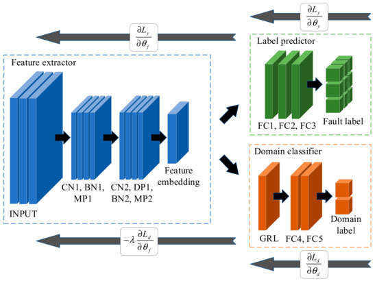
Figure 1.
The structure of DANN.
The specific network structural parameters of DANN are shown in Table 1. Sample features are extracted through the convolution layer, followed by batch standardization and maximum pooling layers, and a dropout layer is added after the second convolution operation to improve the robustness of the network. Gy label classifier is composed of three full connection layers. The number of neurons in the first two full connection layers is 100, and the number of neurons in the last full connection layer is 9, because there are 9 fault types. The domain classifier Gd is composed of a GRL and two full connection layers to perform domain classification on the generated features and determine whether the samples belong to the source domain or the target domain. Therefore, the last full connection layer has two neurons.

Table 1.
Network structural parameters of DANN.
During training, DANN optimizes the parameters θf and θy of feature extractor Gf and classifier Gy by minimizing the loss of tag classifier and feature extractor:
Meanwhile, DANN optimizes its parameter θd by maximizing the loss of Gd domain classifier:
Like the generative adversarial networks, the two steps alternately train the network parameters.
GRL is to facilitate the realization of the above minimum and maximum game process. In the forward-propagation process, GRL is an identity mapping:
In the back-propagation process, the gradient is reversed by multiplying by a negative identity matrix I:
Thus, the above two training processes can be combined into one objective function:
Among them, the Ly(∙,∙) is the loss of the label classifier, Ld(∙,∙) is the loss of the domain classifier, Lyi, and Ldi is the i—the corresponding training sample losses.
2.2. Fault Diagnosis Based on DANN
It is difficult to collect fault signals in operational rotor, and network training of deep learning requires many datasets. Therefore, the time domain signal is resampled to expand the existing dataset. Sample resampling is shown in Figure 2. Sample resampling is to divide a time domain signal into several small samples in chronological order, and there is some signal overlap between each sample, so that the correlation between small samples of time domain signal can be retained. After resampling the samples, the time domain signal is mapped on a time-frequency diagram by STFT.
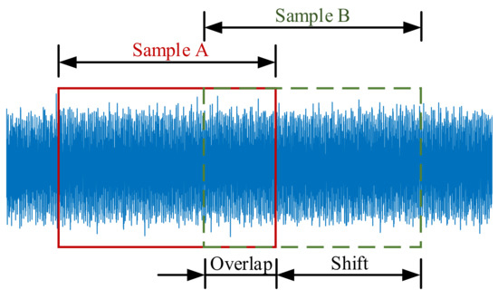
Figure 2.
Overlapping sampling diagram.
The DANN fault diagnosis process proposed in this paper is shown in Figure 3. The original source domain fault vibration signals and target domain fault vibration signals were overlapping sampling and STFT to obtain the dataset required for DANN training. The source domain dataset is divided into training and validating datasets, the target domain dataset is divided into training and testing datasets, the samples in the training and validating datasets are labeled, while the testing dataset is unlabeled. The obtained time-frequency diagram is decoded into a 256 × 256 × 3 vector and standardized for feature generation. Data standardization helps to reduce the training time of the data model and improve the accuracy of the network. The calculation formula is x* = (x − μ)/σ. Where μ is the mean value of sample RGB three-channel. σ is the standard deviation of sample RGB three-channel.
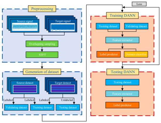
Figure 3.
Diagnostic flow chart.
The preprocessed time-frequency diagrams from training and validating datasets were input to the feature generator to extract the features. The label predictor discriminates the labels of the samples according to the generated features, and the domain classifier is used to distinguish whether the samples come from the source domain or the target domain. The network parameters θf, θy and θd were modified according to the loss of label predictor and domain classifier. After the training, the unlabeled samples in the testing dataset were predicted to evaluate the accuracy of fault diagnosis.
3. Case I: Simulated Gas Generator Rotor
In this section, a simulated gas generator rotor model is established. Vibration signals under different coupling faults are obtained through simulation, and they are divided into source domain and target domain according to different nodes to verify the proposed method.
3.1. Modeling of Gas Generator Rotor
The simulated gas generator rotor is shown in Figure 4a, which is mainly composed of a five-stage wheel and a center rod. Externally, from left to right, the compressor one-level disk, two-level disk, three-level disk, centrifugal impeller, and gas turbine disk are pressed and fixed by the internal central rod. The support is a rolling bearing located at both ends of the rotor.
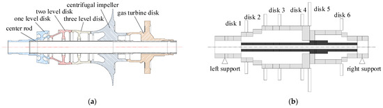
Figure 4.
The simulated gas generator rotor: (a) structural diagram; (b) finite element model.
The node division of the finite element model of the simulated gas generator rotor is shown in Figure 4b, in which the plates of the compressor one-level, two-level, and three-level disks are simplified into disks 1–3, respectively. The gas turbine disk is simplified to disk 6. Considering the large size of the centrifugal impeller disk, the axial distribution distance is long and uneven, so it is simplified into two disks, namely disk 4 and disk 5. Considering the moment of inertia and gyro effect of disks 1–6, it is simplified as concentrated mass point. Which is applied to nodes 6, 9, 11, 13, 14 and 18 of the beam elements, respectively. The center rod (dark) is divided into 15 axis segments with 16 nodes. According to the actual mating relationship of the gas generator rotor, nodes 5, 14, 15, and 20 of the five-stage disk beam model are rigidly connected with nodes 1, 9, 10, and 16 of the center rod, respectively. To sum up, the established finite element model of gas generator simulation rotor has 36 axis segments and 38 nodes.
The finite element model of gas generator simulation rotor is established by a Timoshenko beam element. The basic step is to obtain the element matrix of shaft segment and disk by energy method combined with Lagrange equation, and then assemble the element matrix obtained. Refer to Appendix A for detailed modeling process. Under the rotation speed of 12,000 rpm, the responses of rotor under different coupling faults are obtained by simulation: imbalanced and misaligned coupling faults, imbalanced and static eccentric coupling faults, imbalance and rubbing coupling faults. Set different values of imbalance at disk 1: 20 × 10−5 kg·m, 100 × 10−5 kg·m and 200 × 10−5 kg·m. The imbalance size indicates the severity of the fault, and apply the resulting imbalance force to the node of disk 1. Node 1 of simulated gas generator rotor is connected to the coupling, and the resulting misalignment force is applied to node 1. In practical engineering, due to the influence of machining accuracy, assembly error, and gravity, there is a certain degree of static eccentricity between the support and the rotor, which produces static eccentric force at the support. When assembling the rotor system, when the vibration amplitude of the rotor exceeds the clearance, rubbing fault will occur between the rotor and stator. A gap is added at disk 5, and when the response of disk 5 reaches the rubbing gap, a rubbing force is applied to it. Where F ∊ {Fe, Frub, Fmis, Fse} represents the external forces under different faults, Fe represents the imbalanced excitation force, Frub represents the rubbing force, Fmis represents the misalignment force, Fse represents the static eccentricity oil-film force, Fb represents the rolling bearing force, q represents the generalized displacement, and the rotor dynamic equation is obtained:
The Newmark-β method was used to solve the motion differential equations of rotor system Equation (7). The algorithm has the characteristics of easy convergence and fast computing speed. Since SFD oil-film force and rolling bearing force both introduce nonlinear terms, other loads on the rotor system often also have nonlinear characteristics, so the Newton–Raphson method should be combined to solve iteratively.
3.2. Generation and Expansion of Dataset
The total duration of each fault signal is 5 s, the sampling frequency is 200,000 and the displacement response length is 1,000,000 points. Due to the influence of various nonlinear external excitation during the calculation of each fault, the initial rotor is in an unstable state. It enters stable simple string vibration about 0.2 s later. Therefore, resampling-starting position is taken 1s, and a small sample is taken every 0.1 s, with the length of each small sample being 20,000 points; 5000 points overlap between the two adjacent small samples, as shown in Figure 2. Each fault is resampled to 100 small samples and the obtained time domain signals of the left support are shown in Figure 5, Figure 6 and Figure 7.
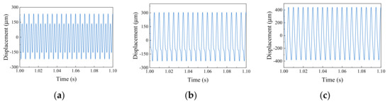
Figure 5.
Imbalanced and misaligned coupling faults: (a) value of imbalance 20 × 10−5 kg·m; (b) value of imbalance 100 × 10−5 kg·m; (c) value of imbalance 200 × 10−5 kg·m.
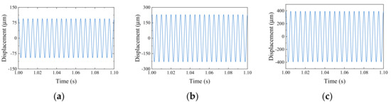
Figure 6.
Imbalanced and static eccentric coupling faults: (a) value of imbalance 20 × 10−5 kg·m; (b) value of imbalance 100 × 10−5 kg·m; (c) value of imbalance 200 × 10−5 kg·m.
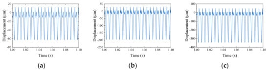
Figure 7.
Imbalance and rubbing coupling faults: (a) value of imbalance 20 × 10−5 kg·m; (b) value of imbalance 100 × 10−5 kg·m; (c) value of imbalance 200 × 10−5 kg·m.
The time-frequency diagram of samples obtained after overlapping sampling were processed by STFT. The hamming window size is 5999, the sample signals are divided into 5 parts, and the overlap points of resampling are 187. The frequency range of the drawing was in the symmetric interval [−1000, 1000]. The time-frequency diagrams of node 2 and node 22 obtained by STFT are shown in Figure 8, Figure 9 and Figure 10. For the 9 coupling faults of the simulated gas generator rotor, the signals supported on the left side (node 2) are used as the source domain dataset, and the signals supported on the right side (node 22) are used as the target domain dataset. There are some differences between the time-frequency diagrams of the same fault samples in the source domain and the target domain, and some similarities between the time-frequency diagrams of different fault samples in the source domain and the target domain. The source and target domains contain 9 fault types, and each fault type contains 100 samples. The 80% samples in source are taken as training dataset, the remaining 20% as validation dataset, and the 20% in target domain are taken as training dataset, and remaining 80% as testing dataset. The training dataset consists of 80% source domain and 20% target domain. By training a large number of source domain samples and a small number of target domain samples, the fault diagnosis effect of the testing dataset of target domain is evaluated.
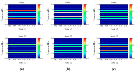
Figure 8.
Time-frequency diagram of imbalanced and misaligned coupling faults: (a) value of imbalance 20 × 10−5 kg·m. (b) value of imbalance 100 × 10−5 kg·m. (c) value of imbalance 200 × 10−5 kg·m.
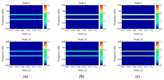
Figure 9.
Time-frequency diagram of imbalanced and static eccentric coupling faults: (a) value of imbalance 20 × 10−5 kg·m; (b) value of imbalance 100 × 10−5 kg·m; (c) value of imbalance 200 × 10−5 kg·m.
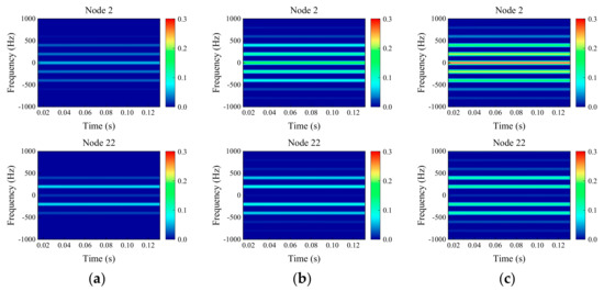
Figure 10.
Time-frequency diagram of imbalanced and rubbing coupling faults: (a) value of imbalance 20 × 10−5 kg·m; (b) value of imbalance 100 × 10−5 kg·m; (c) value of imbalance 200 × 10−5 kg·m.
3.3. Results and Analysis
Figure 11 shows a comparison of the same fault signal plotted in time domain diagram, frequency domain diagram by FFT, and time-frequency diagram by STFT. Nine kinds of fault signals are processed into three sample graphs in Figure 11, which are respectively used as datasets to train the DANN model. Stochastic gradient descent (SGD) optimizer has been selected as the optimizer of DANN, and initial learning rate is 0.0001, batch size is 32, maximum number of training iterations (epochs) is 1000, and the iteration of each epoch is 45. This experiment is implemented on the computer with one Nvidia GeForce GTX 3060Ti GPU, one AMD Ryzen 5 5600X of 3.7 GHz, and 16 GB memory.
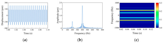
Figure 11.
Comparison of fault signal processing results: (a) time domain diagram; (b) frequency domain diagram; (c) time-frequency diagram.
Accuracy, precision, recall, and F1 score were selected as model-measurement standards. The training results of different diagrams are shown in Table 2. It can be seen from the results that the time-frequency diagram has the best fault diagnosis accuracy of 100%. Other model-measurement standards, such as precision, recall, and F1 score are also 100%. The time-frequency diagram combines time domain information with frequency domain information to amplify the characteristics of different fault samples, then achieving better training results.
Table 2.
The training results of different diagrams.
As shown in Figure 12, the results of the target dataset are displayed in a confusion matrix. The accuracy of fault label prediction of the time domain diagram is the lowest, and the accuracy of fault label prediction of the time-frequency diagram is 100%.
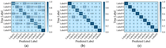
Figure 12.
Confusion matrix of the target dataset: (a) time domain diagram; (b) frequency domain diagram; (c) time-frequency diagram.
The training process of the time-frequency diagram is shown in Figure 13. With the increase in epochs, the accuracy of the training and validating datasets of fault label classifiers keeps rising, and gradually approaches 100% and becomes stable in 200 epochs, indicating that the fault diagnosis model gradually learns the signal characteristics of 9 types of fault labels and can correctly judge fault labels according to the characteristics. The values of precision, recall, and F1 score also gradually approach 100%. Under the action of GRL, the higher the accuracy of domain discriminator, the more difficult the model finds it to distinguish data from source domain or target domain, which proves that the fault diagnosis model successfully projects the features of source domain and target domain into the same feature space. As can be seen from the loss diagram, the loss decreases gradually with the increase in epochs, and the model keeps updating parameters in the direction of reducing the difference between source domain and target domain.
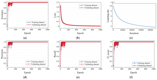
Figure 13.
The training process of time−frequency diagram: (a) accuracy of training process; (b) loss of training process; (c) learning rate of training process; (d) precision of training process; (e) recall of training process; (f) F1 score of training process.
When the number of target domain samples in the training dataset increases, for example, 50% of the training dataset is source domain samples and the remaining 50% is target domain samples, the hyperparameter training is still adopted. The training results are shown in Table 3. By comparing Table 2 and Table 3, it can be seen that with the increase in the target domain samples in the training dataset, the accuracy, precision, recall, and F1 scores all increased.
Table 3.
Types of faults.
As shown in Figure 14, the results of the target dataset are displayed in a confusion matrix. It can be seen from Figure 14c that the identification accuracy of the fault diagnosis model for 9 types of fault time-frequency diagrams is 100%, which is significantly better than the other two diagrams and has good fault identification accuracy. By comparing Figure 12 and Figure 14, it can be seen that with the increase of the target domain samples in the training dataset, the accuracy, precision, recall, and F1 scores all increased.
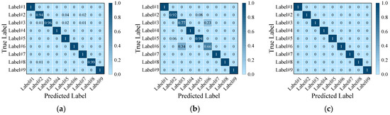
Figure 14.
Confusion matrix of the target dataset, when 50% of the training dataset is target domain samples: (a) time domain diagram; (b) frequency domain diagram; (c) time-frequency diagram.
The feature embedding of source and target domain from DANN with t-SNE [29] for both two datasets are visualized in Figure 15, and different fault types are indicated by different color symbols. T-SNE can visualize the high-dimensional data by mapping samples from the original feature space to two-dimensional space. Compared with the results of source domain Figure 15a,c and target domain Figure 15b,d, it shows obvious clustering and separability between source domain and target domain, which is sufficient to show that the proposed network can reliably perform cross-domain fault diagnosis when there are fewer available samples. The same fault labels of the source and target domains that do not pass feature mapping and those that pass feature mapping are projected to the same region, indicating that the same fault labels of the source and target domains are similar to some extent.
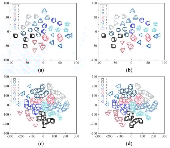
Figure 15.
T−SNE visualization of fault features: (a) time-frequency signal of the source domain; (b) time-frequency signal of the target domain; (c) feature embedding of the source domain derived from DANN; (d) feature embedding of the target domain derived from DANN.
3.4. Verification of Method Robustness
In order to simulate the rotor vibration signal under actual working conditions, appropriate noise was added to the response, and the formula of SNR was as follows [30]
where Noise(t) is a Gaussian noise function. A is the amplitude of noise signal and the value of A is the standard deviation of q. Then the response signal after adding noise is
The imbalanced and misaligned coupling faults are taken as an example. When the SNR is 50 dB, 20 dB, and 10 dB, the response obtained is shown in Figure 16. The setting of hyperparameters is consistent with the noiseless time-frequency diagram of training. The epoch is 500, iteration is 45, and batch size is 32. The SGD optimizer with an initial learning rate of 0.0001 is adopted. The training process of different SNR is shown in Figure 17. The smaller the SNR value, the slower the accuracy increases and the slower the loss decreases, but the accuracy of signals with different SNR all approach 100%. It can be seen that the method used in this paper has high fault diagnosis accuracy and high robustness for TIM on the simulated gas generator rotor.
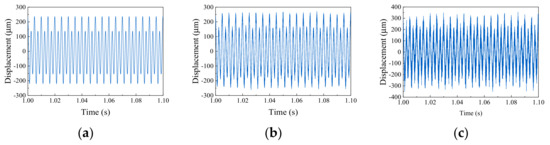
Figure 16.
Responses of different SNR: (a) time domain diagram (SNR = 50 dB); (b) time domain diagram (SNR = 20 dB); (c) time domain diagram (SNR = 10 dB).
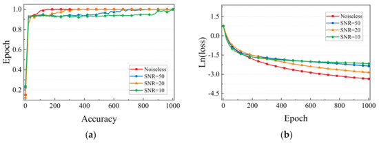
Figure 17.
The training process of different SNR: (a) the accuracy of different SNR; (b) the ln(loss) of different SNR.
4. Case II: Experimental Rig of Rotor
4.1. Arrangement of Experiment
The rotor experimental data under different faults were collected by the experimental rig of rotor (as shown in Figure 18). The vibration signals of rotor were collected by data acquisition and analysis system. Using two eddy current sensors, respectively arranged on the left side and right side of A shaft, and measuring the horizontal displacement of rotor, the signal through the signal cable into the rotor machine controller, the signal disposal controller sends signals to dynamic signal analyzer within the data collection device to realize analogue signal resistance to mix the steps, such as filtering and A/D conversion. Then, the digital signal is converted into on that can be processed by the upper analysis software. Finally, the digital signal is uploaded to the computer analysis software and the vibration signal is processed.
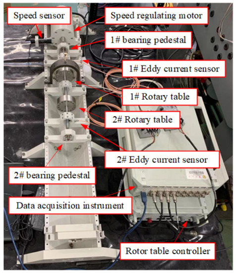
Figure 18.
Experimental rig of rotor.
4.2. Generation and Expansion of Dataset
The parameters of the rotor fault experiment are shown in Table 3. The fault types of rotor are mainly divided into imbalance, rubbing, and misalignment, and are further subdivided into three fault types with different degrees of eccentric mass blocks.
In this experiment, a screw was screwed at the left disk, and 0.2 g, 1 g, and 2 g screws were used to represent different fault types at different degrees. The rotation speed was 2000 rpm, and the sampling frequency was 1000 Hz. Thus, imbalanced fault signals were collected.
In high-speed and high-pressure centrifugal compressor rotating machinery, in order to improve unit efficiency, the shaft seal, interstage seal, oil-seal clearance, and blade-top clearance are often designed to be small to reduce gas leakage. However, too small a clearance will not only cause hydrodynamic excitation but also cause friction between rotor and stationary parts. The rubbing fault in this experiment is to add a bolt at the bracket above the disk, and the gap is controlled between 1 mm and 2 mm. Set the speed to 1800 rpm and sampling frequency to 1000 Hz.
The main cause of misalignment fault of rotor is the thermal deformation of large rotor due to heavy load, self-load, and long-term high-temperature environment. The misalignment of the simulated rotor in the experiment means that the journal is misaligned in the deflection bearing, that is, the other end of the rotor is added under the support position, so that the rotating shaft has a certain inclination. Set the speed to 2500 rpm and sampling frequency to 25,600 Hz.
Due to the limited number of samples of 9 kinds of time domain signals collected by the two sensors, time domain signals are taken as a sample every 50 revolutions. According to the relationship between sampling frequency and speed, the length of each sample for each fault can be obtained, as shown in Table 4; 100 samples were taken for each fault type. In order to expand the dataset and solve the problem of insufficient training dataset, resampling fault signals in the time domain was carried out. For measured vibration data, each sample was sampled from the last quarter of the previous sample, so that there was a quarter overlapping between samples. The dataset obtained after overlapping sampling is shown in Figure 19, Figure 20 and Figure 21.
Table 4.
Length of sampling faults signal.
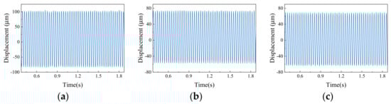
Figure 19.
Imbalanced faults: (a) value of imbalance 2.5 × 10⁻⁵ kg·m; (b) value of imbalance 5 × 10⁻⁵ kg·m; (c) value of imbalance 10 × 10−5 kg·m.
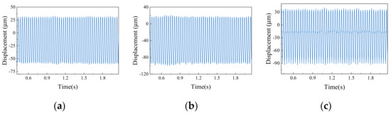
Figure 20.
Rubbing faults: (a) value of imbalance 2.5 × 10⁻⁵ kg·m; (b) value of imbalance 5 × 10⁻⁵ kg·m; (c) value of imbalance 10 × 10−5 kg·m.
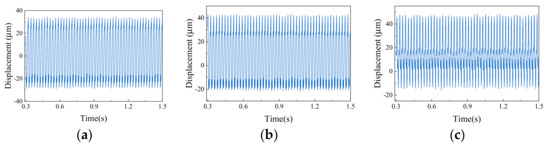
Figure 21.
Misaligned faults: (a) value of imbalance 2.5 × 10⁻⁵ kg·m; (b) value of imbalance 5 × 10⁻⁵ kg·m; (c) value of imbalance 10 × 10−5 kg·m.
The resampled time domain signal is processed by STFT, and the window function is a Hamming window. The sample signal is divided into 5 parts. Therefore, the size of the Hamming window is 300, 330, and 6140 respectively, and the corresponding overlapping points are 9, 10, and 191. The frequency range of the graph is symmetric [−200, 200], so that the characteristics between different fault types are more distinct. The frequency range with small- or even zero-power spectrum value is removed. The time-frequency diagrams of the left sensor and the right sensor obtained by STFT and the STFT results of 9 kinds of fault signals are shown in Figure 22, Figure 23 and Figure 24.
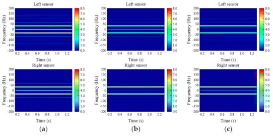
Figure 22.
Time-frequency diagram of imbalanced faults: (a) value of imbalance 2.5 × 10⁻⁵ kg·m; (b) value of imbalance 5 × 10⁻⁵ kg·m; (c) value of imbalance 10 × 10−5 kg·m.
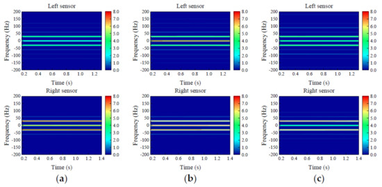
Figure 23.
Time-frequency diagram of rubbing faults: (a) value of imbalance 2.5 × 10⁻⁵ kg·m; (b) value of imbalance 5 × 10⁻⁵ kg·m; (c) value of imbalance 10 × 10−5 kg·m.
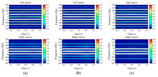
Figure 24.
Time-frequency diagram of misaligned faults: (a) value of imbalance 2.5 × 10⁻⁵ kg·m; (b) value of imbalance 5 × 10⁻⁵ kg·m; (c) value of imbalance 10 × 10−5 kg·m.
4.3. Results and Analysis
In this experiment, there are 9 kinds of faults of two sensors with 100 samples for each fault. The 80% of the 900 samples at the left sensor are used as the source domain training dataset, and the remaining 20% samples are used as the validation dataset. Similarly, 900 samples at the right sensor are taken as the training dataset of the target domain. The 20% samples at the right sensor as the target domains were taken as training dataset, the remaining 80% samples as testing dataset. SGD optimizer has been selected, and initial learning rate is 0.0001, batch size is 32, epochs is 500, the iteration of each epoch is 45. The comparison of fault signal processing results is shown in Figure 25.
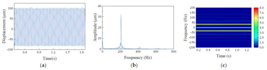
Figure 25.
Comparison of fault signal processing results: (a) time domain diagram; (b) frequency domain diagram; (c) time−frequency diagram.
It can be seen from Table 5 that the accuracy of the three diagrams is above 90%, while the precision, recall, and F1 scores of the time-frequency diagram are the highest, followed by the time-domain diagram and the frequency domain diagram. It can be seen that the time-frequency diagram can obtain better fault diagnosis results.
Table 5.
Results of different diagrams.
4.4. Transfer Learning between Experimental Dataset and Simulation Dataset
The fault data obtained from the actual rotor structure are limited, and sometimes the fault data are not easy to measure. The previous examples are TIM, and this section will verify the feasibility of TDM. The simulation dataset of the simulated gas generator rotor is taken as the source domain and the experimental dataset measured by the experimental rig of rotor is taken as the target domain. Both the samples of source domain and target domain are time-frequency diagrams. The source domain and target domain are divided into training dataset, validating dataset and testing dataset. The training dataset consists of 80% simulation dataset and 20% experimental dataset. The remaining 20% of the simulation dataset is the validating dataset. The remaining 20% of the experimental dataset is the testing dataset. The training dataset consisted of 900 samples, 720 simulation samples and 180 experimental samples. The validation dataset contains 180 simulation samples. The testing dataset consisted of 720 experimental samples. The hyperparameters of network remain constant. The training results can be seen from Figure 26. that the accuracy, precision, recall and F1 score has approached at 100% after about 200 epochs and fluctuated in a small range.
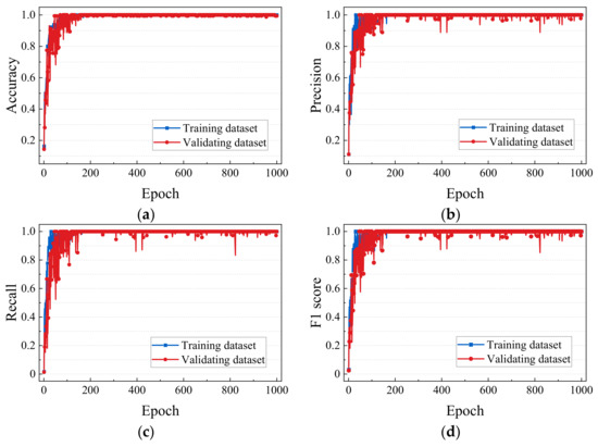
Figure 26.
The process of training: (a) the results of accuracy; (b) the results of precision; (c) the results of recall; (d) the results of F1 score.
The fault diagnosis results of source domain and target domain are displayed in the confusion matrix, as shown in Figure 27. The accuracy of source domain is 100%. Then the accuracy of the target domain is 100%, except for Label#8 which is 99%. T−SNE results of source domain and target domain are shown in Figure 28. Some original samples of source domain overlap that of target domain. Through feature embedding derived from DANN, different faults are distinguished, and the same faults of source domain and target domain are mapped to the same region.
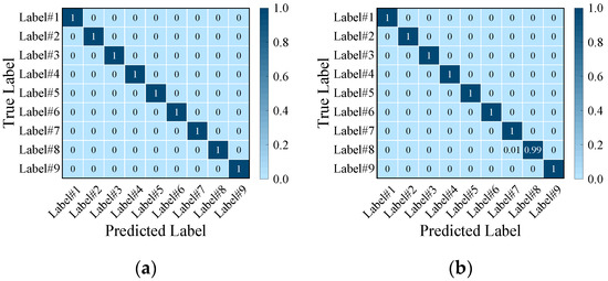
Figure 27.
Confusion matrix: (a) source domain; (b) target domain.
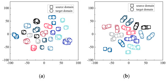
Figure 28.
T−SNE visualization of fault features: (a) original signal; (b) feature embedding derived from DANN. Squares represent the source domain and circles represent the target domain. Color represents different fault labels.
5. Conclusions
In this paper, the fault diagnosis method of rotor based on DANN with time-frequency diagram by STFT is proposed, one-dimensional fault vibration signal feature extraction and fault type of discriminant together, the fault diagnosis model is obtained by the source domain sample, and the target domain of failure types of samples, the knowledge of the source domain transfer to the target domain for the aim of rotor fault diagnosis. According to different types of rotor fault signals, appropriate sample length, window function type, window function width and sample overlap points corresponding to STFT are selected. In order to improve the robustness and accuracy of fault diagnosis, the method of overlapping sampling is adopted to expand the dataset. The influence of different values of SNR on the diagnosis results was compared according to the noise signals in actual working conditions. According to the experimental rig of rotor and simulated gas generator rotor, the following conclusions are drawn:
- (1)
- STFT can well combine information of the time domain with information of the frequency domain, distinguish the characteristics of different fault signals, and effectively improve the accuracy of DANN fault diagnosis model.
- (2)
- The DANN fault diagnosis methods proposed in this paper can obtain good fault diagnosis for simulated gas generator rotor and experimental investigations. This method can transfer the limited information of source domain to the target domain, and diagnose the fault in the target domain which lacks training knowledge. Both TIM and TDM have been implemented in this paper.
- (3)
- The method presented in this paper can still obtain good fault diagnosis accuracy for the signals disturbed by noise and has high robustness.
- (4)
- The simulation data of the simulated gas generator rotor dataset is used as the source domain, and the experimental dataset measured by the experimental rig of rotor is used as the target domain. The network of the training simulation dataset is effectively transferred to the experimental dataset, which is TDM, and the problem of insufficient fault samples in the actual rotor structure is solved.
Author Contributions
Conceptualization, D.J.; funding acquisition, D.J.; methodology, J.L. and Z.W.; resources, J.L.; software, Y.X.; validation, Y.X. and Z.W.; writing—original draft, Y.X.; writing—review & editing, J.L., Z.W., D.Z. and D.J. All authors have read and agreed to the published version of the manuscript.
Funding
This research was funded by the National Natural Science Foundation of China (No. 11602112), Natural Science Research Project of Higher Education in Jiangsu Province (20KJB460003), the QingLan Project, National Natural Science Foundation of China (52005100), Natural Science Foundation of Jiangsu Province (BK20190324), Jiangsu Association for Science and Technology Young Talents Lifting Project (TJ-2022-043), the Fundamental Research Funds for the Central Universities and Zhishan Youth Scholar Program of SEU (2242021R41169).
Institutional Review Board Statement
Not applicable.
Informed Consent Statement
Not applicable.
Data Availability Statement
Not applicable.
Conflicts of Interest
The authors declare that there are no conflict of interest regarding the publication of this paper.
Appendix A. Modeling of the Simulated Gas Generator Rotor
The support is a rolling bearing, and assuming that the ball bearings are evenly distributed and roll at the same speed, ignoring the centrifugal force, the supporting force of the rolling bearing can be expressed as [31]
where α is the contact angle of the rolling bearing, θi is the angular position of the i-th ball bearing of the rolling bearing, ωcage is the angular velocity of the ball revolution, satisfying
where Ri and Ro are the radius of inner and outer rings respectively, Cb is the Hertz contact stiffness between ball and inner and outer rings, n is the number of ball bearings, μ is the clearance of rolling bearing, H(·) represents Heaviside function: when the value in brackets is greater than 0, the function value is 1. This function returns to zero when the value in parentheses is less than or equal to zero.
The imbalance of rotor is described by the magnitude of imbalance mass m and its position (eccentricity distance e and phase φ). Satisfaction of imbalance
The rotor imbalanced excitation force is proportional to the square of the angular velocity
When the imbalance of the i-th rotor node appears (i = 1,2…), the imbalanced excitation vector at this node is [32]
The imbalanced excitation matrix vector Fe can be obtained by assembling the imbalanced excitation matrix at each node.
The left end of the rotor is connected with the coupling, corresponding to node 1 of the finite element model.
Figure A1a shows the misaligned deflection angle of the coupling relative to node 1 of the rotor finite element model. The center distance between node 1 and the other node of the coupling is Z3 and the deviation angle is θ3. The force and torque exerted by the coupling on node 1 have been indicated in the figure, where Mz2 = −Mz1 = −Tq, and Tq is the torque transmitted by the coupling. Since the flexible coupling mainly transmits torque, its axial force can be ignored, so Fz2 = −FZ1 = 0. The remaining load on node 1 is [33]
where kb is the torsional stiffness of the coupling.
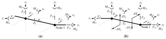
Figure A1.
Analysis of misalignment geometry and force: (a) deflection angle of misalignment; (b) parallel of misalignment.
For the parallel of misalignment, as is show in Figure A1b, the center line of the coupling and the center line of the rotor are parallel to each other, but offset by a certain distance in the plane perpendicular to the axial direction. The force and torque on node 1 are
where θ1, θ2, φ1 and φ2 are coupling misalignments, which can be expressed as
When misalignment failure occurs, the generalized load fmis of node 1 is
Since misalignment failure occurs only at node 1 of the finite element model, the misalignment term corresponding to other nodes is zero, and the misalignment force Fmis received by the rotor system can be obtained.
Circumferential rub means that the rotor may contact the stator at any position within one rotation. Its mechanical model is shown in Figure A2. Assuming that the radial deformation of the stator is linear, and the friction between the rotor and the stator conforms to Coulomb’s friction law, then the rubbing force is
where kc is the radial stiffness of the stator, f is the Coulomb friction coefficient between the rotor and stator, and δ0 is the rotor clearance. The tangential friction PT is proportional to the positive pressure PN between the rubbing contact surfaces. e is the radial displacement of the rotor. The rubbing force occurs only when e exceeds the stator gap. Convert the rubbing force to the Cartesian coordinate system
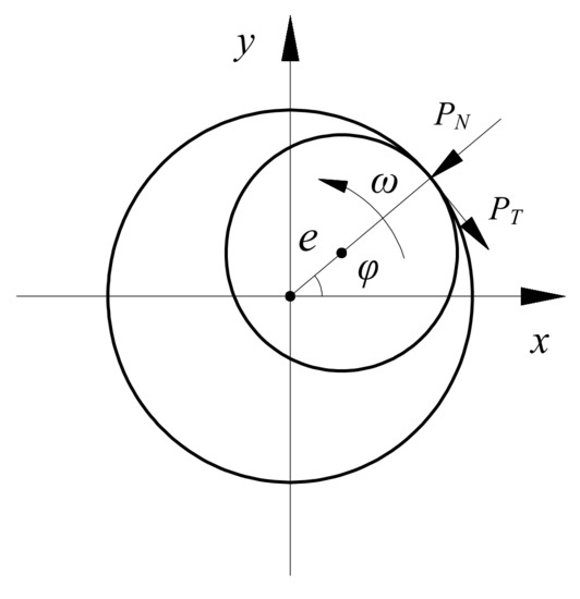
Figure A2.
Mechanical model of rubbing.
Then, sinφ = y/e, cosφ = x/e, and substitute Equation (A10) into Equation (A11), can be obtained
The rubbing force vector frub was applied to the nodes with rubbing in the finite element model, and the position of the nodes without rubbing was replaced by the zero vector to obtain the rubbing force matrix Frub of the system.
The characterization formula of SFD oil-film force was derived under static eccentricity, and the calculation model was established first [34], as shown in Figure A3. In order to represent the position of static eccentricity, a rectangular coordinate system was established with the center of the outer ring Ob as the origin, and the axial direction was denoted as z, the horizontal direction perpendicular to the axis was denoted as x, and the vertical direction was denoted as y. For convenience, static eccentricity is assumed to occur in the positive direction of the X-axis, and the initial position of the inner ring center Oj0 is offset from the distance es relative to the origin Ob, and its coordinates are assumed to be (xe, ye). In the working condition of this section, the coordinate is (xe, 0), but the former is still used as the coordinate of the static eccentric position in order to make the derived characterization formula more applicable.
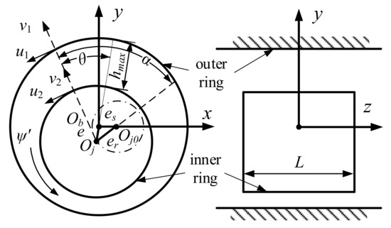
Figure A3.
Calculation model of static eccentric SFD.
Assuming that the fluid is incompressible and the dynamic viscosity is constant, according to the generalized Reynolds equation of SFD, the Reynolds equation of SFD in the state of static eccentricity is
where p(θ, z) represents the pressure distribution in SFD, θ is the oil-film starting angle, calculated from the maximum oil film thickness. μ is the viscosity of lubricating oil; h is the local oil-film thickness. c is the oil-film gap, and the actual eccentricity is ε = e/c. Since Oj precession around Oj0, ψ is the precession angle. α is the included angle between the oil-film starting angle and the relative dynamic eccentricity line, α and θ have the following relationship
The short bearing hypothesis solution Equation (A13). Then integrated along the axial direction and the circumferential direction, the radial force and tangential force of oil film are obtained
where I1, I2 and I3 are Sommerfeld integrals
μ is the viscosity of lubricating oil. h is the local oil-film thickness. R is the SFD radius. Since the oil-film gap is minimal relative to the inner and outer rings, R = Rb = Rj.
It is assumed that the static eccentricity occurs at the left and right supporting nodes, and the static eccentricity oil-film force of the system is denoted as Fse, and the position of other nodes is replaced by the zero vector.
References
- Yang, C.Y.; Wu, T.Y. Diagnostics of gear deterioration using EEMD approach and PCA process. Measurement 2015, 61, 75–87. [Google Scholar] [CrossRef]
- Ren, Z.; Zhou, S.; Chunhui, E.; Gong, M.; Li, B.; Wen, B. Crack fault diagnosis of rotor systems using wavelet transforms. Comput. Electr. Eng. 2015, 45, 33–41. [Google Scholar] [CrossRef]
- Unal, M.; Onat, M.; Demetgul, M.; Kucuk, H. Fault diagnosis of rolling bearings using a genetic algorithm optimized neural network. Measurement 2014, 58, 187–196. [Google Scholar] [CrossRef]
- Ji, Y.; Wang, H. A Revised Hilbert–Huang Transform and Its Application to Fault Diagnosis in a Rotor System. Sensors 2018, 18, 4329. [Google Scholar]
- Yan, X.; Liu, Y.; Zhang, W.; Jia, M.; Wang, X. Research on a Novel Improved Adaptive Variational Mode Decomposition Method in Rotor Fault Diagnosis. Appl. Sci. 2020, 10, 1696. [Google Scholar] [CrossRef]
- Yan, X.; Jia, M. Application of CSA-VMD and optimal scale morphological slice bispectrum in enhancing outer race fault detection of rolling element bearings. Mech. Syst. Signal Process. 2019, 122, 56–86. [Google Scholar] [CrossRef]
- Pang, B.; Tang, G.; Zhou, C.; Tian, T. Rotor Fault Diagnosis Based on Characteristic Frequency Band Energy Entropy and Support Vector Machine. Entropy 2018, 20, 932. [Google Scholar] [CrossRef]
- Lee, C.-Y.; Zhuo, G.-L. Effective Rotor Fault Diagnosis Model Using Multilayer Signal Analysis and Hybrid Genetic Binary Chicken Swarm Optimization. Symmetry 2021, 13, 487. [Google Scholar] [CrossRef]
- Kavitha, S.; Bhuvaneswari, N.S.; Senthilkumar, R.; Shanker, N.R. Magnetoresistance sensor-based rotor fault detection in induction motor using non-decimated wavelet and streaming data. Automatika 2022, 63, 525–541. [Google Scholar] [CrossRef]
- Zhao, X.; Jia, M.; Ding, P.; Yang, C.; She, D.; Liu, Z. Intelligent Fault Diagnosis of Multichannel Motor-Rotor System Based on Multimanifold Deep Extreme Learning Machine. IEEE-Asme Trans. Mechatron. 2020, 25, 2177–2187. [Google Scholar] [CrossRef]
- Tamilselvan, P.; Wang, P. Failure diagnosis using deep belief learning based health state classification. Reliab. Eng. Syst. Saf. 2013, 115, 124–135. [Google Scholar] [CrossRef]
- Krizhevsky, A.; Sutskever, I.; Hinton, G.E. ImageNet Classification with Deep Convolutional Neural Networks. Commun. Acm 2017, 60, 84–90. [Google Scholar] [CrossRef]
- Gu, J.; Wang, Z.; Kuen, J.; Ma, L.; Shahroudy, A.; Shuai, B.; Liu, T.; Wang, X.; Wang, G.; Cai, J.; et al. Recent advances in convolutional neural networks. Pattern Recognit. 2018, 77, 354–377. [Google Scholar] [CrossRef]
- Jiang, G.; He, H.; Yan, J.; Xie, P. Multiscale Convolutional Neural Networks for Fault Diagnosis of Wind Turbine Gearbox. IEEE Trans. Ind. Electron. 2019, 66, 3196–3207. [Google Scholar] [CrossRef]
- Ince, T.; Kiranyaz, S.; Eren, L.; Askar, M.; Gabbouj, M. Real-Time Motor Fault Detection by 1-D Convolutional Neural Networks. IEEE Trans. Ind. Electron. 2016, 63, 7067–7075. [Google Scholar] [CrossRef]
- Abdeljaber, O.; Avci, O.; Kiranyaz, S.; Gabbouj, M.; Inman, D.J. Real-time vibration-based structural damage detection using one-dimensional convolutional neural networks. J. Sound Vib. 2017, 388, 154–170. [Google Scholar] [CrossRef]
- Zhu, X.; Hou, D.; Zhou, P.; Han, Z.; Yuan, Y.; Zhou, W.; Yin, Q. Rotor fault diagnosis using a convolutional neural network with symmetrized dot pattern images. Measurement 2019, 138, 526–535. [Google Scholar] [CrossRef]
- Lu, C.; Wang, Z.; Zhou, B. Intelligent fault diagnosis of rolling bearing using hierarchical convolutional network based health state classification. Adv. Eng. Inform. 2017, 32, 139–151. [Google Scholar] [CrossRef]
- Yan, X.; She, D.; Xu, Y.; Jia, M. Deep regularized variational autoencoder for intelligent fault diagnosis of rotor–bearing system within entire life-cycle process. Knowl.-Based Syst. 2021, 226, 07142. [Google Scholar] [CrossRef]
- Wang, J.; Ji, S.; Han, B.; Bao, H.; Jiang, X. Deep Adaptive Adversarial Network-Based Method for Mechanical Fault Diagnosis under Different Working Conditions. Complexity 2020, 2020, 6946702. [Google Scholar] [CrossRef]
- Wu, Z.H.; Jiang, H.K.; Zhao, K.; Li, X.Q. An adaptive deep transfer learning method for bearing fault diagnosis. Measurement 2020, 151, 107227. [Google Scholar] [CrossRef]
- Lu, W.N.; Liang, B.; Cheng, Y.; Meng, D.S.; Yang, J.; Zhang, T. Deep Model Based Domain Adaptation for Fault Diagnosis. IEEE Trans. Ind. Electron. 2017, 64, 2296–2305. [Google Scholar] [CrossRef]
- Wen, L.; Gao, L.; Li, X.Y. A New Deep Transfer Learning Based on Sparse Auto-Encoder for Fault Diagnosis. IEEE Trans. Syst. Man Cybern.-Syst. 2019, 49, 136–144. [Google Scholar] [CrossRef]
- Lei, Y.G.; Yang, B.; Jiang, X.W.; Jia, F.; Li, N.P.; Nandi, A.K. Applications of machine learning to machine fault diagnosis: A review and roadmap. Mech. Syst. Signal Process. 2020, 138, 106587. [Google Scholar] [CrossRef]
- Guo, L.; Lei, Y.; Xing, S.; Yan, T.; Li, N. Deep Convolutional Transfer Learning Network: A New Method for Intelligent Fault Diagnosis of Machines With Unlabeled Data. IEEE Trans. Ind. Electron. 2019, 66, 7316–7325. [Google Scholar] [CrossRef]
- Pan, S.J.; Yang, Q. A Survey on Transfer Learning. IEEE Trans. Knowl. Data Eng. 2010, 22, 1345–1359. [Google Scholar] [CrossRef]
- Li, C.; Zhang, S.; Qin, Y.; Estupinan, E. A systematic review of deep transfer learning for machinery fault diagnosis. Neurocomputing 2020, 407, 121–135. [Google Scholar] [CrossRef]
- Ganin, Y.; Ustinova, E.; Ajakan, H.; Germain, P.; Larochelle, H.; Laviolette, F.; Marchand, M.; Lempitsky, V. Domain-Adversarial Training of Neural Networks. J. Mach. Learn. Res. 2016, 17, 2030–2096. [Google Scholar]
- van der Maaten, L.; Hinton, G. Visualizing Data using t-SNE. J. Mach. Learn. Res. 2008, 9, 2579–2605. [Google Scholar]
- Xiong, T.; Gu, Z. Observer-Based Fixed-Time Consensus Control for Nonlinear Multi-Agent Systems Subjected to Measurement Noises. IEEE Access 2020, 8, 174191–174199. [Google Scholar]
- Chen, G. A New Rotor-Ball Bearing-Stator Coupling Dynamics Model for Whole Aero-Engine Vibration. J. Vib. Acoust.-Trans. Asme 2009, 131, 061009. [Google Scholar] [CrossRef]
- de Castro, H.F.; Cavalca, K.L.; Nordmann, R. Whirl and whip instabilities in rotor-bearing system considering a nonlinear force model. J. Sound Vib. 2008, 317, 273–293. [Google Scholar] [CrossRef]
- Ma, H.; Wang, X.; Niu, H.; Wen, B. Oil-film instability simulation in an overhung rotor system with flexible coupling misalignment. Arch. Appl. Mech. 2015, 85, 893–907. [Google Scholar] [CrossRef]
- Bei, G.; Ma, C.; Sun, J.; Ni, X.; Ma, Y. Porous Media Leakage Model of Contact Mechanical Seals Considering Surface Wettability. Coatings 2021, 11, 1338. [Google Scholar]
Publisher’s Note: MDPI stays neutral with regard to jurisdictional claims in published maps and institutional affiliations. |
© 2022 by the authors. Licensee MDPI, Basel, Switzerland. This article is an open access article distributed under the terms and conditions of the Creative Commons Attribution (CC BY) license (https://creativecommons.org/licenses/by/4.0/).