6.2. Multi-Objective Structural Optimization
The main method to deal with the multi-objective structural optimization problem of CDPM is the weighted coefficient method [
33,
53,
54]. However, the weighted coefficient method has three shortcomings: first, the weight coefficients are determined according to the designer’s subjective intention; second, the weight coefficients are difficult to quantify accurately; third, a single weight coefficient is difficult to represent all design intents due to the infinite selections of weight coefficients. In addition to the weighted coefficient method, there are some other multi-objective structural optimization methods for CDPMs, such as the enumeration method [
55] and tabular method [
56]. However, these methods are not objective, because the optimal criteria are determined by designers subjectively. Accordingly, we apply the ideal-point method to tackle the multi-objective structural optimization problem.
Process of the ideal-point method: first, three optimization objectives are conducted to obtain the optimal solution with regard to each objective; secondly, the solution spaces of the three objectives are normalized to the interval [0, 1], and the optimal value of each objective is normalized to “0”; finally, the minimum sum of the distances between the three optimization objectives and “0” is taken as the optimization objective, namely the “ideal point”. The PIEAMIGA was implemented with MATLAB programming language and executed on a notebook computer with a 2.2 GHz Intel Core I5-5200U CPU and a 12 G RAM.
6.2.1. The Optimal Value and Worst Value of Single-Objective Optimization
Since the GA itself does not have the ability to deal with constraints, it is necessary to transform the constrained optimization problem into unconstrained optimization problem, which can be realized through the penalty function method. Thus, the fitness function of the optimization object
with regard to design variable vector
is as follows:
where
is the fitness degree function, and
.
is a transfer function.
is a large positive number and is used as the penalty factor.
The parameters of SGA and PIEAMIGA are listed in
Table 2. The simulation parameters of the optimization model are shown in
Table 3. According to the site and installation conditions, the range of the length
and width
of the horizontal projection rectangle of pulleys are [80, 90] m and [70, 80] m, respectively; the range of the height of the pulleys’ points is [25, 30] m. The range of the mass of the CPTDS is [20, 50] kg. The MSTS is a 70 m × 60 m × 22 m cuboid, whose volume
is 92,400
. Based on the parameters listed in
Table 2 and
Table 3, PIEAMIGA and SGA are programmed by MATLAB to find the optimal solution and value with regard to three optimization objects separately, which are listed in
Table 4. The worst values with regard to the single optimization object are also listed in
Table 4.
It can be seen from
Table 4 that the optimal solution obtained by PIEAMIGA is better than that obtained by SGA. Workspace volume increases by 8.52%, the first-order natural frequency increases by 9.73%, and the impulse exerted by tensions on the CPTDS to CPTDS is reduced by 10.08%. Although three modules are added into PIEAMIGA based on SGA, the computing time of PIEAMIGA increases by 4.48% compared with that of SGA because the multi-island GA adopts the parallel mechanism, and operations in each island are performed in parallel. It also can be seen from
Table 4 that PIEAMIGA has a stronger global search ability as the result of the adaptive crossover and mutation rate.
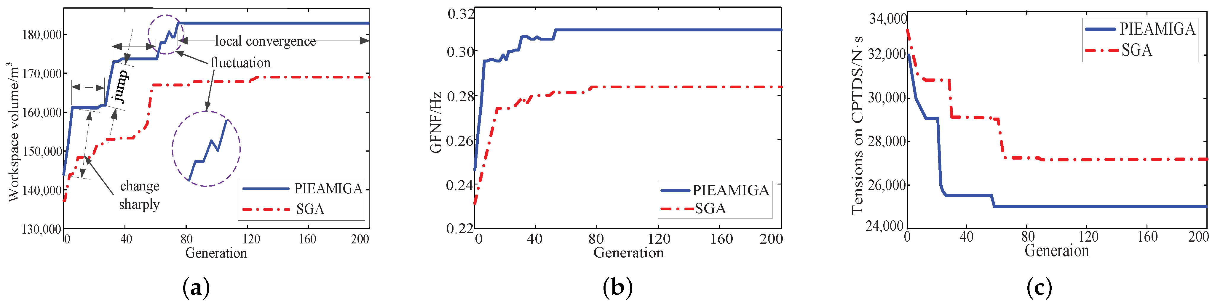
The convergence processes of each objective by the PIEAMIGA and SGA are shown in
Figure 14. In the early stage of evaluation, the optimal solution changes rapidly due to the randomness of population and great differences between individuals, which is a sharply changed line in
Figure 14a. With the progress of evolution, the number of excellent individuals in the population gradually increases; thus, the change of optimal solution slows down, and the local convergence appears, which is a horizontal line in
Figure 14. Furthermore, the process of local convergence is prolonged gradually as the result of the increasing proportion of excellent individuals in the population.
Thus, the change of the optimal solution is not as violent as in the initial stage, and the length of the horizontal line is gradually longer with the increase in generation of evolution. There exist a jump after the local convergence process on the curve because the optimal solution jumps out of a local optimal solution and evolves towards a better optimal solution. It is inevitable that the performance of the offspring will be degraded compared with the parent because the new individuals are not always better than the parent individuals, which is a fluctuating line in
Figure 14a. It can also be seen from
Figure 14 that PIEAMIGA shows the better “climbing” (downhill) ability with the progress of evolution, and thus the gap between the two curves becomes increasingly larger. Finally, PIEAMIGA converges to the global optimal solution while SGA can only converge to the sub-optimal solution.
Figure 15a shows that the workspace boundary extends outwards after using PIEAMIGA and that the volume increases by 14,425
compared to SGA.
Figure 15b shows that the first-order natural frequency on the horizontal section of workspace that the height
z is 6 m has significantly increased after using PIEAMIGA, and the GFNF is increased by 0.0452 Hz compared to SGA.
Figure 15c shows that the impulse sum to the CPTDS has decreased significantly after using PIEAMIGA, and the impulse sum is decreased by 2792 N·s compared to SGA.
6.2.2. Multi-Objective Optimization Based on the Ideal Point Approach
In the previous sections, we performed structural optimization with regard to the three optimization objectives, respectively. However, we want to optimize the three optimization objectives simultaneously, i.e., the largest workspace, the highest first-order nature frequency and the smallest impulse on CPTDS exerted by tensions. Mathematically, it is a multi-objective optimization problem and will be solved by using the ideal-point method.
Since the physical meaning of the three optimization objectives is different, it is necessary to normalize the three optimization objectives , and , respectively. Thus, the three optimization objects become continuous functions in the [0,1] interval, and the multi-objective function is uniform in dimension. The maximum and minimum values of each optimization objective need to be normalized.
As shown in
Table 4, for
,
,
; for
,
Hz,
Hz; for
,
N·s,
N·s. Thus, we can find three objectives after normalization:
According to the definition of the ideal-point method, the minimum sum of the distances between the three objective function and the three ideal points is taken as the optimization objective, and the linear and nonlinear constraints proposed in previous are taken as the optimization constraints:
6.3. Results and Discussion of Multi-Objective Structural Optimization
According to the simulation parameters listed in
Table 3 and
Table 4, the multi-objective structural optimization is conducted by real-coded PIEAMIGA in the MATLAB environment. The results are listed in
Table 5. It can be seen that the three optimization results are balanced, none of which is dominant, while others perform poorly.
Figure 16 shows the DFFW corresponding to the optimal solution
, which completely contains the MSTS, and thus the filming work can be successfully completed.
Figure 17 and
Table 6 illustrate the relationship of the workspace volume
with the pulley point height
and the mass of CPTDS
when the optimization variables
and
are fixed. In this case,
and
. The pulley height
is not positively correlated with volume of workspace
. It can be known from the curved surface that the volume is small at both ends and large in the middle. It can be seen from
Table 6 that the workspace volumes are about the same when the pulley height is equal to 27 and 28 m, and thus the maximum value is near
m.
Generally speaking, the higher the pulley height is, the larger the volume is. However, the tension range is also a decisive factor of workspace. With the increase in height , the angle between the tangent line at the cable end and the direction of gravity decreases; thus, the cable tension must be increased to balance the gravity. The increase in height will cause an increase in the length and weight of the cable, and thus an increase in the cable tension. Thus, it is possible that the tensions exceed the upper limit , leading to a decrease in the workspace that is mainly located in the area near the pulley point close to the upper surface of the workspace.
Relatively speaking, the relationship between the mass of CPTDS and the workspace volume is obvious, which has two characteristics: (1) Positive correlation. The light mass of CPTDS may give rise to the decrease in cable tension, or even less than the lower limit . The reduced volume of workspace is mainly located at the boundaries of the workspace, where the area of the cable tension is relatively small. (2) At the beginning of the curve, the increase is obvious; however, at the end of the curve, the change is small.
When the mass is small, increasing the mass of CPTDS will significantly enhance the cable tension so that many position points that originally do not meet the lower limit satisfy the lower limit again. Therefore, the volume of workspace increases. However, when the mass increases to a certain extent, the minimum tension at most of the points have been greater than . Therefore, the increase in the workspace volume is limited.
Figure 18 shows the spatial distribution of the first-order natural frequency corresponding to the “ideal point” on three horizontal sections of the workspaces at different heights, i.e.,
z = 5 m,
z = 15 m and
z = 25 m. Clearly, the higher the height along the
z axis is, the higher the natural frequency is. Since the camera robot belongs to the suspended CDPM, the four pulley points are all above the CPTDS. Therefore, the higher the height along
z axis is, the shorter the cable length is. According to Equation (
25), the shorter the cable length, the higher the natural frequency of the camera robot. Similarly, there is always a long cable when the CPTDS at one of the four corners of the workspace; hence, the first-order natural frequency of the camera robot will be smaller, leading to a downward sharp corner.
Figure 19 shows the minimum value of the first-order natural frequency on the different horizontal sections of the workspace with different heights, which are significantly improved compared with those shown in
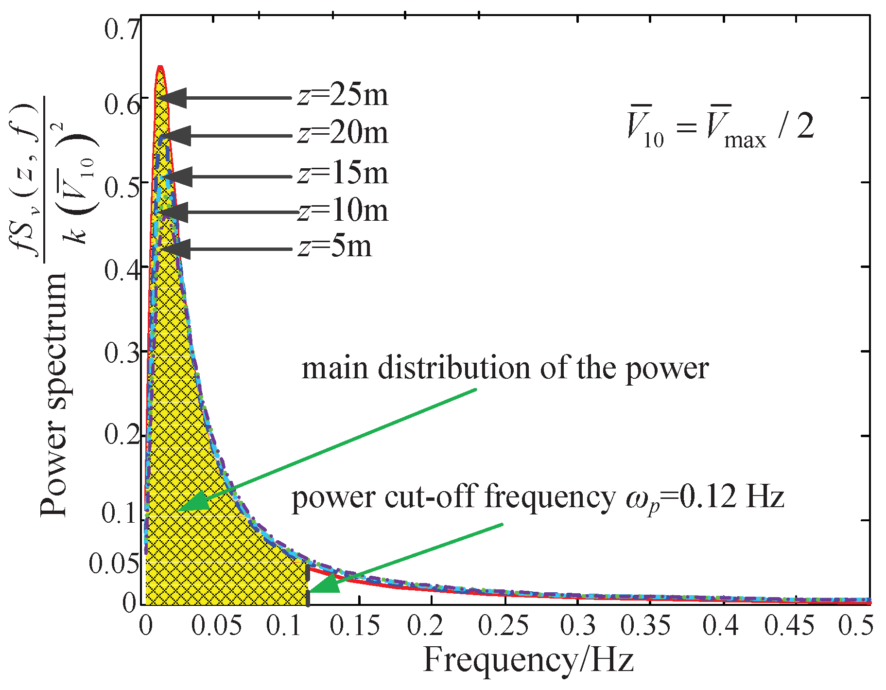
Figure 10. The minimum first-order natural frequency on each horizontal section all exceeds 0.12 Hz. At
z = 5 m, the minimum first-order natural frequency is equal to 0.13 Hz. Although it has been improved, it is still close to the energy truncation frequency
= 0.12 Hz. Therefore, it is still vulnerable to wind disturbance. Thus, some measures are essential to enhance the first-order natural frequency of the camera robot, such as the stiffness improvement and tension regulation.
Figure 20 and
Table 7 show the relationship of GFNF with the pulley point height
and the mass of CPTDS
when the optimization variables
and
are fixed. In this case,
and
. The relationship between GFNF and
is not proportional, but exhibits the characteristics of “high at both ends, low in the middle”. It can be concluded from Equation (
21) that the critical factor of determining the GFNF is the length of the cable. On the one hand, the smaller the height
is, the smaller the length of the cable is. Thus, the frequency is larger when
= 25 m; However, on the other hand, the decrease in height
will lead to the decrease in the height of workspace, lead to losing some points in workspace.
Since the cable length at these “losing point” is shorter, the first-order natural frequency is larger. Therefore, the whole level of the natural frequency in the workspace will decrease after losing these points. Hence, the contradiction between them determines that the value of GFNF is larger when is equal to the maximum or minimum height and smaller when is in the middle height. The relationship between the mass of CPTDS and GFNF is very obvious. The greater the mass is, the lower the frequency is. We can observed that the GFNFs are the same when the pulley height at 27 m and 28 m. We can also draw the conclusion that the GFNF is more sensitive to the pulley height than the mass of the CPTDS.
Figure 21 shows the impulse applied on the CPTDS and the accelerations of the CPTDS corresponding to the optimization solution following the sampling locus shown in
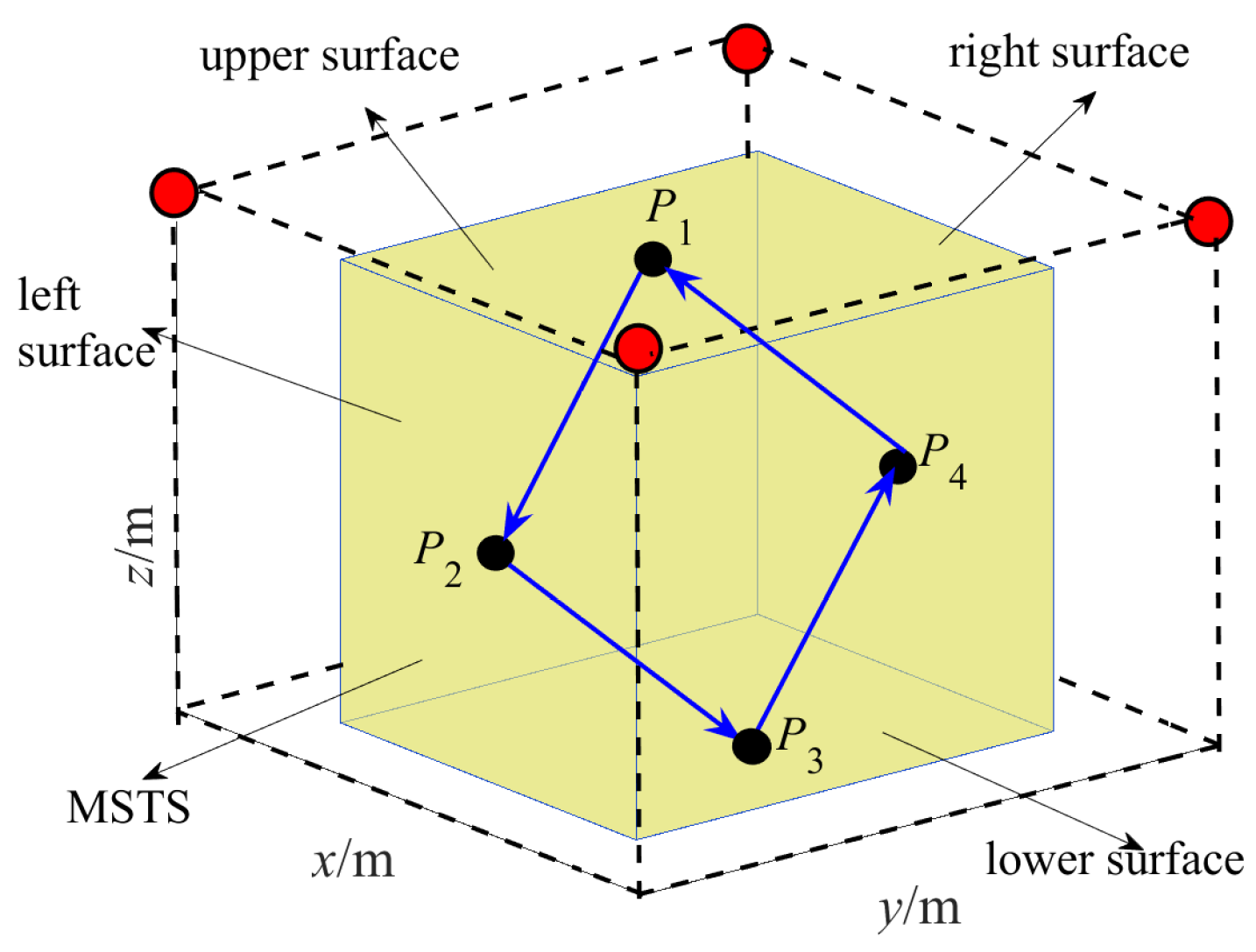
Figure 11. Since every straight line segment of the locus is planned by a quintic polynomial, the acceleration curve is a cubic curve, and the value of acceleration at each point change motion direction of the locus is 0. It can be seen that the impulse is larger in the time point with larger acceleration, reflecting the tensions exert a large impulse on the CPTDS at this time point. The maximum value appears at
t = 15 s, when the CPTDS moves near the point
and is close to the lower surface of the workspace.
Therefore, the cable length and tension are larger than those at the rest points and thus the impulse. It can be observed that the curve is not completely symmetrical on both sides with as the center. However, the left side is larger and the right side is smaller. As the segment is on the left side of and the motion direction is consistent with the direction of gravity, the tension is larger; the motion direction of the segment on the right side of is contrary to the gravity direction, and therefore the tension is smaller. Thus, the impulse on the segment is larger than that on the segment . Similarly, the impulse applied on the CPTDS on the segment is larger than that on the segment .
Figure 22 and
Table 8 show the relationship of the impulse sum on the CPTDS along the sampling locus with the pulley point height
and the mass of CPTDS
when the optimization variables
and
are fixed. In this case,
and
. There is a positive correlation of the impulse sum with the pulley point height
and the mass of CPTDS
. The higher the pulley point height
and the greater the mass
of the CPTDS are, the greater the impulse sum will be. In addition, it can be observed from
Table 8 that the impulse sum linearly increases with increasing of the pulley point height and the mass of the CPTDS.


