Article

Dynamic Modeling, Workspace Analysis and Multi-Objective Structural Optimization of the Large-Span High-Speed Cable-Driven Parallel Camera Robot

1
Department of Intelligent Manufacturing Engineering, School of Mechatronic Engineering, Xi’an Technological University, Xi’an 710021, China
2
Key Laboratory of Electronic, Equipment Structure Design, Xidian University, Xi’an 710071, China
3
School of Mechanical Engineering, Xi’an University of Science and Technology, Xi’an 710054, China
*
Author to whom correspondence should be addressed.
Machines 2022, 10(7), 565; https://doi.org/10.3390/machines10070565
Submission received: 6 June 2022 / Revised: 8 July 2022 / Accepted: 11 July 2022 / Published: 14 July 2022
(This article belongs to the Special Issue New Frontiers in Parallel Robots)

Abstract

:
Since most of the cable-driven parallel manipulators (CDPMs) are small in dimension or low in speed, the self-weight or inertia of the cable is neglected when dealing with the problems of kinematics, dynamics and workspace. The cable is treated as a massless straight line, and the inertia of the cable is not discussed. However, the camera robot is a large-span high-speed CDPM. Thus, the self-weight and inertia of the cable cannot be negligible. The curved cable due to the self-weight is modeled as a catenary to accurately account for its sagging effect. Moreover, the dynamic model of the camera robot is derived by decomposing the motion of the cable into an in-plane motion and an out-plane motion, based on which an iterative-based tension distribution algorithm and a workspace generation algorithm are presented. An optimization model is presented to simultaneously improve the workspace volume, anti-wind disturbance ability and impulse of tensions on the camera and pan–tilt device system (CPTDS) by selecting the proper optimal variables under the linear and nonlinear constraints. An improved genetic algorithm (GA) is proposed, and the simulation results demonstrate that the improved GA offers a stronger ability in global optimization compared to the standard genetic algorithm (SGA). The ideal-point method is employed to avoid the subjective influence of the designer when performing the multi-objective optimization, and a remarkable improvement of the performance is obtained through the optimization. Furthermore, the distribution characteristics of the optimization objects are studied, and some valuable conclusions are summarized, which will provide some valuable references in designing large-span high-speed CDPMs.

1. Introduction

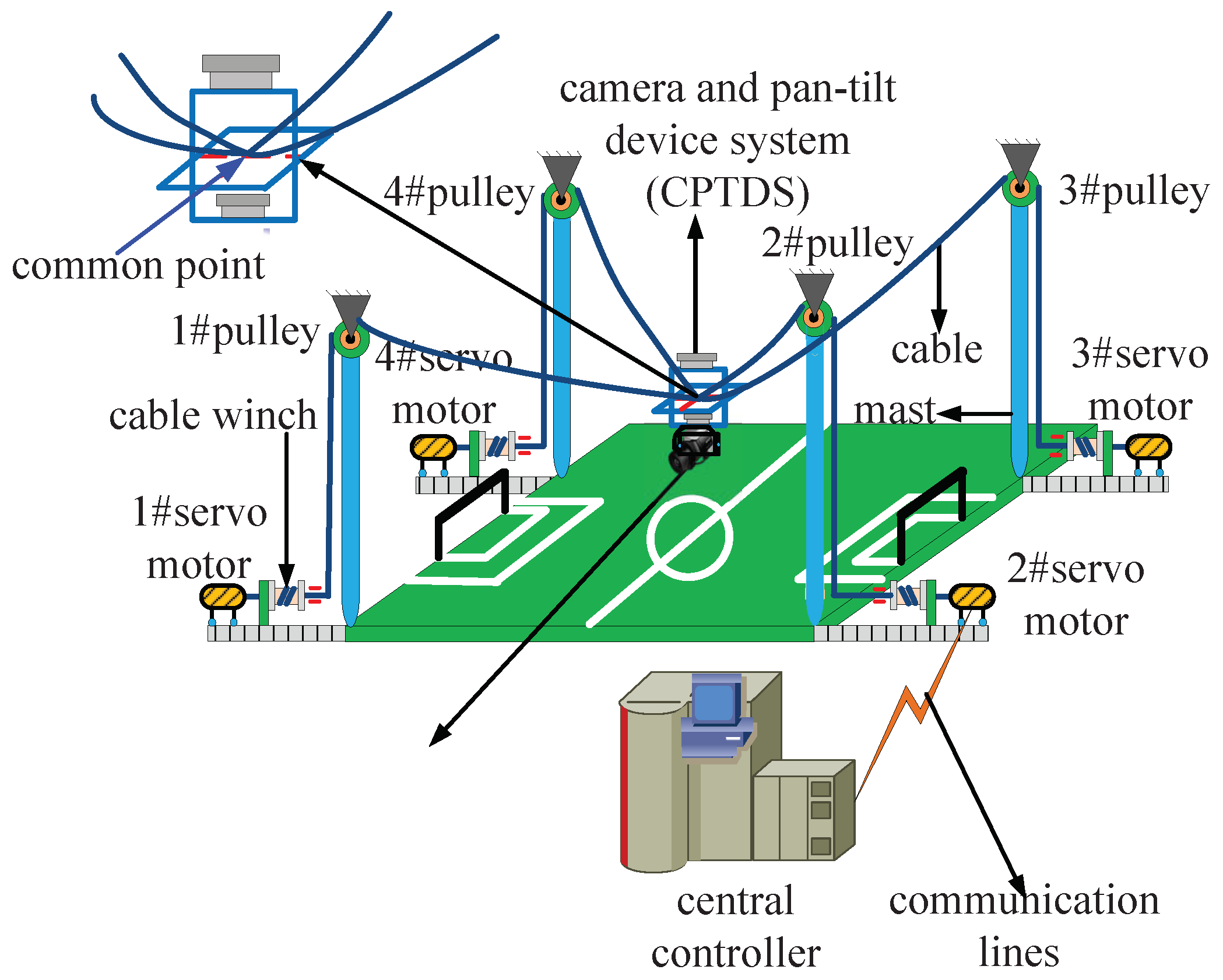
The cable-driven parallel camera robot (camera robot for short, see Figure 1) is a type of CDPM (cable-driven parallel manipulator) consisting of four computer-driven servo motors that enable the controlled release of four cables that act in parallel on an end-effector, i.e., the CPTDS (camera and pan–tilt device system). The camera robot can take pictures and videos with an aerial view that conventional cameras would have difficulty in realizing [1], making it the best candidate for aerial panoramic photographing in big venues, such as stadiums, football fields, theaters, etc.
There have existed some commercial camera robots, e.g., Skycam, Spidiercam and Cablecam [2], which can also be applied in agricultural remote sensing [3] and traffic monitoring [4] and film production [5]. A camera robot is a typical of large-span high-speed CDPM with redundant actuation [6], whose performance is largely determined by its structural parameters [7,8].
The essence of structural optimization is to establish the mapping relationships between optimal variables and optimization objects. Determining an optimal structure of a CDPM meeting a set of optimization objectives is generally challenging, which can be solved by formulating a constrained optimization problem. There has been plenty of prior work in the structural optimization of CDPMs, which employ various optimization objects, such as workspace size [9], condition number of Jacobian matrix [10], tension factor [11,12], stiffness [13,14,15], avoiding collision of cables [16,17], manipulability [18] and the maximum acceptable horizontal distance [19].
However, most of the above optimization methods belong to traditional optimization methods, such as the simplex method, interval analysis, Dynamic-Q, grouped coordinate descent and enumeration method, which are sensitive to initial values and easily fall into local optimums, leading to a failure to obtain a global optimal solution. Until now, many optimal methods have been developed to overcome this difficulty. Genetic algorithms (GA) are an intelligent optimization method offering a powerful global search ability and can effectively escape from local optimums compared to the traditional optimization method, causing it to be a mainstream structural optimization approach of CDPMs.
Li et al. proposed a GA-based multi-objective optimization method to obtain the best global dexterity index and overall stiffness index of a planar three degrees of freedom (DOF) CDPM [20]. Jamwal et al. developed a GA-based multi-objective optimization method to conduct the optimal design of a cable-driven ankle rehabilitation robot using the minimum global condition number, the maximum workspace utilization index and the minimum cable tension norm as optimal objectives [21]. Arsenault et al. used GA to optimize the geometry of planar CDPMs with four cables with the objective of reaching a desired pre-stress stable wrench-closure workspace [22].
Bahrami et al. optimized the workspace volume, kinematic performance indices and actuating energy of a spatial CDPM by means of GA, [23]. Amine and Hamida investigated the structural optimization of a cable-driven upper limb rehabilitation robot (LAWEX) based on GA, where the objectives were the simultaneous minimization of the robot size and the tensions in the cables [24,25]. Nevertheless, cables in these studies were all treated as massless straight lines without considering the self-weights, which are only suited to small-dimensional CDPMs.
There are two aspects that require attention in the structural optimization of the camera robots: large-span and high-speed motion. For the large-span CDPMs, the sagging effect due to the self-weight of the cable cannot be neglected [26,27], as the profile of the cable is no longer a straight line but a curve. Generally, the deformed curve under self-weight can be described as a catenary or a parabola [28,29].
Jiang et al. optimized the dimensional parameters of a under-restrained six-DOF CDPM (URPM4-3R3T) with workspace size as the objective function [30]. Yao et al. obtained the better dimension parameters for a CDPM with four cables used for the feed supporting system of the five-hundred-meter aperture spherical radio telescope (FAST) to meet the workspace requirements [31]. Tang et al. optimized dimensional parameters for constructing a CDPM with six cables for FAST based on the sensitivity design method and three tension performance evaluating functions [32].
Du determined the structural parameters to simultaneously improve the stiffness and dexterity of large workspace CDPMs [33]. Wei presented an approach on the stability analysis of cable-driven parallel robots considering cable mass based on cable tensions and stiffness matrix condition numbers [34]. However the motions of manipulators are low-speed or quasi-static, and thus the dynamics of the manipulators were not considered.
The highest speed of the camera robot that is known currently is up to 9 m/s [35]. Hence, the maneuverability of the camera robot due to the high-speed motions must be considered. Barrette et al. proposed a notion of a dynamic workspace of CDPMs on the conditions of the dynamic and tension for a planar CDPM [36]. Kawamura et al. developed a high-speed manipulation (FALCON-7) by using a CDPM and studied its dynamics based on the vector closure condition [37].
Gagliardini et al. proposed an improved dynamic feasible workspace considering the inertia of a moving platform, external wrenches applied on the moving platform and the Coriolis forces corresponding to a constant moving platform twist concurrently [38]. Yu et al. determined the dynamic workspace of a camera robot by taking the intersection of workspaces with accelerations at different directions [35] and studied the relationships between the reachable area of the workspace bottom and heights of masts. Kieu et al. developed a modified kinematic equation considering cable nonlinear tension and analyzed the wrench-feasible workspace at various motion accelerations [39]. However, the self-weights of the cables in these studies were all negligible. In our preliminary work, the dynamic modeling and cable tension distribution considering the self-weight and inertia of the cable were simultaneously investigated [1,40], which could provide a theoretical basis for the structural optimization of the camera robot. However, the essence of the tension distribution algorithm in our preliminary work is a multi-dimensional parameter optimization problem, which is time-consuming and has the risk of failure in determining the optimization parameters.
Thus, the algorithm is not fit for CDPMs whose number of cables is much greater than the DOF of the end-effector, which limits the scope of applications. In this paper, the dynamical model of the camera robot is established considering the self-weight and inertia of the cable simultaneously. Furthermore, the tension distribution algorithm is simplified based on the iterative idea to reduce the computing time and computational complexity. Based on the dynamical model, a dynamic workspace generating approach is presented. On the basis of the dynamic workspace, the structural optimization of the camera robot is studied applying a GA, and the ideal-point method is used to deal with multi-objective problems.
The organization of the rest of the paper is as follows: Section 2 establishes the dynamic model of the camera robot by employing the catenary model of the cable and considering the inertia of the cable. Section 3 proposes an iterative-based optimization algorithm based on the dynamic model to determine the tension distribution. Section 4 develops a workspace generation algorithm based on the judging conditions of the dynamic force-feasible workspace. Section 5 presents an optimization model aiming at achieving the maximum workspace volume, anti-wind disturbance and impulse of tensions on CPTDS. Section 6 employs the ideal point method to deal with the multi-objective optimization based on an improved genetic algorithm and studies the distribution characteristics of the optimization objects. Section 7 summarizes our conclusions.

2. Dynamic Model of the Camera Robot

2.1. Description of the Camera Robot

The structure of the camera robot is showed in Figure 1, consisting of a CPTDS driven by four cables in parallel. One end of the cable is connected to the CPTDS, and the other end is wound on the pulley and extends to connect to the cable winch and servo motor. The CPTDS can fly freely in every direction because the cables can be shortened and lengthened through winding driven by four servo motors mounted on the ground, which receive control commands from the central controller.
As shown in Figure 1, the four cables intersect at a common point, and therefore the cables are only responsible for translation. The camera is mounted on a pan–tilt device, which resembles a composite hinge structure. By means of the pan–tilt device, the camera realizes pan (yawing) and tilt (pitching) motion. As a result, the CPTDS can be looked as an ideal mass point P with three translational DOFs, at which the four cables meet. Thus, the position vector P = [ x y z ] T of the point P is expressed in the global fixed frame { o x y z } , and it also denotes the end point of the cable. The camera robot can be categorized to completely restrained positioning mechanisms (CRPMs) [41]—namely, the number of the cables m is equal to DOF of the CPTDS n plus one ( m = n + 1 ).

2.2. Catenary Equation of the Cable

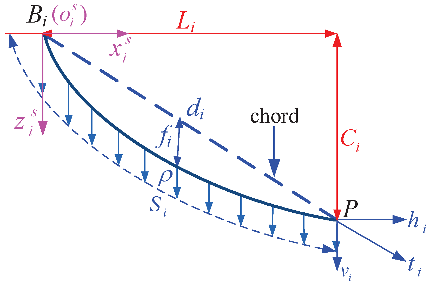
In order to guarantee the stability of the camera robot, the cables must be inextensible and offer high strength. A previous study indicated that a cable can be seen as a catenary under the sag influence. As a consequence, the profile of the cable i ( { i = 1 , 2 , 3 , 4 } ) is a catenary within a vertical plane, noted o i s x i s z i s , is shown in Figure 2. For analysis, the symbols used in Figure 2 are defined as follows: B i = [ B i , x B i , y B i , z ] T denotes the position vector of cable drawing point B i on the pulley in { o x y z } . { o i s x i s z i s } is the local moving frame with the origin o i s attached to B i , and the direction of z i s is straight down.
t i is the tension in the cable i at the end point P, h i is the horizontal component of t i , and v i is the vertical component of t i . L i is the horizontal length of the span of cable i, and C i is the vertical length of the span of cable i. ρ is linear density of the inextensible cable, and m p is the mass of the CPTDS. S i is the length of the cable i, and f i is the sag of cable i at the center of the horizontal span. The catenary equation can be written as follows [42]:
z i s = h i ρ g cosh α i cosh 2 β i x i s l i α i
where g is the gravitational acceleration, and
α i = sinh 1 β i C i / L i sinh β i + β i
β i = ρ L i 2 h i
Equation (1) represents mathematically a family of catenaries. The whole catenary can be determined being given coordinates of arbitrary points on the catenary. Consequently, the length S i of the cable i can be calculated as follows:
S i = L i h i β i ρ l i L i 16 β i e 4 β i 2 α i e 4 β i + 2 α i + 1 2
According to Equation (3), the length of the cable is closely interrelated with the tension. When x i s = L i / 2 , the sag f i can be obtained as follows:
f i = 8 h i sinh β i sinh 1 ρ g C i / 2 h i sinh β i ρ C i g 2 ρ g

2.3. Inertia of the Rapidly Varying-Length Cable

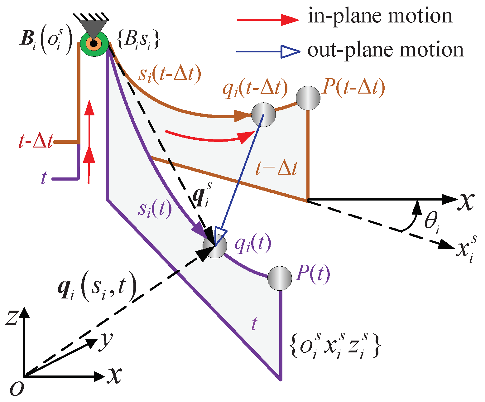
Due to the high-speed motions of the camera robot, the length of cable changes rapidly, leading to the non-negligible inertia of the cable. As shown in Figure 3, q i is a node on cable i with the time-varying curve length s i away from B i , whose position vector can be denoted by q i ( s i , t ) = [ x i y i z i ] T in the global frame { o x y z } . The relationship q i and q i s can be calculated as follows:
q i = Q q i s + B i
where q i s = [ x i s z i s ] T in the local moving frame { o i s x i s z i s } , and Q = cos θ i 0 sin θ i 0 0 1 is the rotation matrix from frame { o i s x i s z i s } to frame { o x y z } , and θ i is the angle between x i s and x.
Since the motion of q i is decomposed to an out-plane motion between the vertical planes and an in-plane motion along the cable as shown in Figure 3, the velocity and acceleration of q i can be calculated by taking the first and second-derivative of q i ( s i , t ) with respect to s i and time t, respectively, in the following expression [1]:
d q i d t = q i t + q i s i s ˙ i d 2 q i d t 2 = 2 q i t 2 + 2 2 q i s i t + 2 q i s i 2 s ˙ i + q i s i s ¨ i
where 2 q i t 2 is yielded by the cable’s out-plane motion and q i s i s ¨ i by the the cable’s in-plane motion; 2 q i s i t and 2 q i s i 2 s ˙ i are yielded by the combination of cable’s in-plane motion and out-plane motion. s ˙ i = d s i / d t , and s ¨ i = d s ˙ i / d t .
Since the cable drawing point B i on the pulley i is attached to the mast, B ˙ i = 0 . Noting that q i s = d i s S i s i and q i t = P ˙ = [ x ˙ y ˙ z ˙ ] T . Thus, the derivatives of q i ( s i , t ) with respect to the curve length coordinate s i can be obtained as follows:
q i s i = s i q i s = Q q i s s i = Q d i s S i = d i S i q i s i t = s i q i t = s i P ˙ 2 q i s i 2 = s i q i s i = Q s i d i s S i = s i d i S i
Moreover, 2 q i t 2 = P ¨ = [ x ¨ y ¨ z ¨ ] T , which is the acceleration of the CPTDS. Substituting Equation (7) into (6), the inertia of the cable i can be found by integrating the whole cable:
I i = ρ 0 S i d 2 q i d t 2 s i = ρ P ¨ S i + 2 P ˙ s ˙ i + d i S i s ˙ i 2 + d i s ¨ i

2.4. Dynamic Equation of the Camera Robot

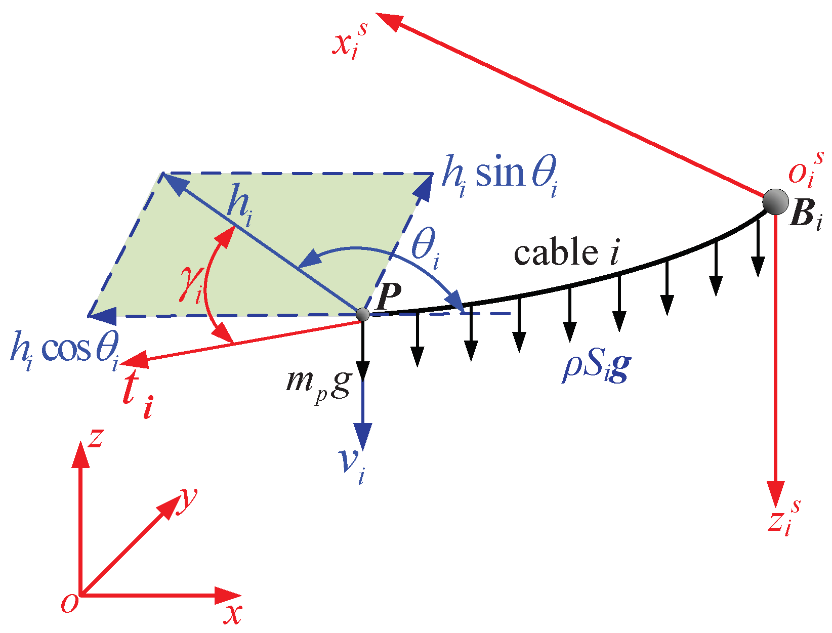
As illustrated in Figure 4, the cable tension t i of the cable i is along the tangential direction of the catenary at the cable end node P. As a consequence, t i can be decomposed into the components that are along the directions of the x, y and z axes, respectively, which can be written in terms of h i cos θ i h i sin θ i h i tan γ i T , where h i is the horizontal component of t i as described in Equation (1) and γ i is the angle between h i and t i . The inertia I i = I i , x I i , x I i , x T is a 3 × 1 vector. W = W x W y W z T is the external force on the CPTDS. The tangent tan γ i at P can be computed as the following equation:
tan γ i = d z i s d x i s x i s = L i = sinh 2 β i α i
Thus, the dynamic equilibrium equation can be written as follows:
m P x ¨ + i = 1 4 I i , x = i = 1 4 h i cos θ i + W x m P y ¨ + i = 1 4 I i , y = i = 1 4 h i sin θ i + W y m P z ¨ + i = 1 4 I i , z = i = 1 4 h i tan γ i i = 1 4 ρ g S i m g + W z
Equation (10) can be further transferred to the following matrix form:
M P ¨ + I ¨ c a b = J h + W + G + G c a b
where M = m p 0 0 0 m p 0 0 0 m p and m p is the mass of the CPTDS. I c a b = i = 1 4 I i , x i = 1 4 I i , y i = 1 4 I i , z T and H = h 1 h 2 h 3 h 4 T . J = cos θ 1 cos θ 2 cos θ 3 cos θ 4 sin θ 1 sin θ 2 sin θ 3 sin θ 4 tan γ 1 tan γ 2 tan γ 3 tan γ 4 is the Jacobian matrix of the camera robot. G = 0 0 m p g T denotes the gravity vector of the CPTDS, G c a b = 0 0 i = 1 4 ρ g S i T is the total gravity vector of the four cables.

3. Iterative-Based Tension Distribution Algorithm

Equation (11) can be further simplified to the following formulation:
JH = F
where F = M P ¨ + I c a b W G G c a b is the generalized external force. As Figure 4 shows, the vertical component of the tension v i = h i tan γ i . Thus, the cable tension t i of cable i can be calculated through the following equation:
t i = h i 1 + tan 2 γ i
The horizontal component h i of t i should subject to the following restraint condition:
h i , min h i h i , max
where the lower bound of the cable tension h i , min is required to keep cable i tight; the upper bound of the cable tension h i , max is defined to account for the the output torque of the servo motor i and the maximum tension that the cable i can withstand without breaking. In this paper, h i , min = h min and h i , max = h max .
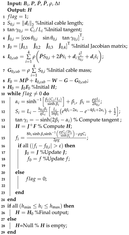
According to Equation (12), it is a non-linear transcendental equation because J and F are associated with H . In this paper, we propose an iterative-based algorithm to determine H , which is different from the algorithm in our previous paper. The algorithm termination condition is when the difference of two sags obtained from adjacent steps is small enough, which could meet after several iterative steps. As a result, although the algorithm in this manuscript does not meet an optimization goal, and the computing time and computational complexity are greatly reduced.
After obtaining H , the cable tension T = t 1 t 2 t 3 t 4 T can be calculated according to Equation (13). It is well-known that the initial values have a significant impact on the iterative method. After several trails, the tensions and lengths of the cables obtained by the massless straight line model of the cable are used as the initial values. Since the profile of the cable is a straight line, the initial sag f 0 = 0 0 0 0 T . ε is a small value and to be used as the threshold of the iterative-based algorithm. Thus, the iterative-based tension distribution algorithm can be summarized as Algorithm 1:
Algorithm 1: Distribution of tensions.
Machines 10 00565 i001

4. Workspace Analysis

4.1. Dynamic Force-Feasible Workspace

There are many workspace criteria proposed to tackle with the influence on the workspace of the unilateral nature of the wrenches (combination of force and moment) applied on the end-effector by cables, among which the wrench-closure workspace (WCW) [43] and wrench-feasible workspace (WFW) [44] are of particular interest. In fact, the WFW is of more practical significance because the cable tensions must be limited within a reasonable range.
There is no moment applied on the CPTDS because this is a mass point. Thus, the camera robot only has a force-feasible workspace (FFW). A position of the end-effector of the CDPM is said to be force-feasible in a particular structure and for a specified set of forces, if the tensions in the cables can counteract any external force of the specified set applied to CPTDS. Liu proposed the generalized determining conditions of WFW/FFW [45] as follows:
(1)
The Jacobian matrix J is full rank.
(2)
The tensions in the cables are all positive and in a definite range.
(3)
The magnitude and direction of the projections of column vectors arbitrarily chosen from the Jacobian matrix J and the external force J are both balanced on a normal vector of the hyperplane determined by J .
In this paper, the dynamic force feasible workspace (DFFW) was applied based on the FFW. For the camera robot, the Jacobian matrix J and generalized external force F have some unique features. On the one hand, the Jacobian matrix J depends not only upon the geometry configuration of the manipulator but also on the tensions and self-weights of cables. On the other hand, the generalized external force F should consist of the inertias of the cables and CPTDS.
Based on the proposed generalized determining conditions of FFW, we can summarize the judging conditions of DFFW, including the direction balance condition (DBC) and magnitude balance condition (MBC). The DBC, which is also the force-closure condition, is given as follows:
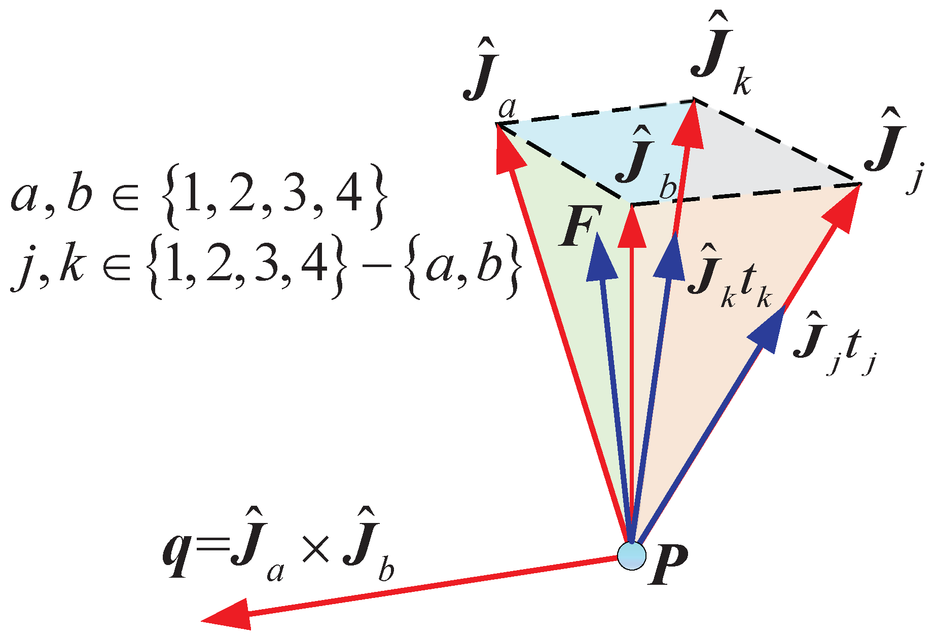
q T F > 0 k : q T J ^ k < 0 q T F < 0 j : q T J ^ j > 0
where q = J ^ a × J ^ b is a unit normal vector of a hyperplane determined by the column vectors of J and pointing towards the exterior of the zonotope as shown in Figure 5. J ^ i = cos θ i sin θ i tan γ i T is the column vector of J . a and b are the subscripts of two linearly independent column vectors arbitrarily chosen from J with a , b 1 , 2 , 3 , 4 ; j and k are the subscripts of the rest column vectors with j , k 1 , 2 , 3 , 4 a , b .
As displayed in Figure 6a, the projections of the tension J ^ j h j (or J ^ k h k ) and the generalized external force F on q are both scalars. Consequently, there always exists a tension J ^ j h j (or J ^ k h k ) to resist the the generalized external force F as long as the signs of q T J ^ j (or q T b m J ^ k ) and q T F are different. However, H ranges from h min to h max . Hence, the components of H J ^ j h j and J ^ k h k are bound with J ^ j h min , J ^ j h max and J ^ k h min , J ^ k h max as shown in Figure 6b. Therefore, the MBC is given as follows:
Γ min Γ max + + q T F Γ min + + q T F Γ max
where Γ min + and Γ max + are the lower and upper limit of the sum of projections of the rest column vectors on the positive direction of q , respectively; Γ min and Γ max are the lower and upper limit of the sum of projections of the rest column vectors on the negative direction of q , respectively. They can be computed as follows:   
Γ min + = q T J ^ j > 0 q T J ^ j h min , Γ max + = q T J ^ j > 0 q T J ^ j h max
Γ min = q T J ^ k < 0 q T J ^ k h min , Γ max = q T J ^ k < 0 q T J ^ k h max
The pre-condition to determine DBC or MBC is the Jacobian matrix J is full rank. Thus, the DFFW can be described as the following set:
P : r a n k ( J ) = 3 q R 3 , q T F > 0 , k : q T J ^ k < 0 Γ min Γ max + + q T F Γ min + + q T F Γ max P : r a n k ( J ) = 3 q R 3 , q T F < 0 , j : q T J ^ j > 0 Γ min Γ max + + q T F Γ min + + q T F Γ max

4.2. Procedure of Generating DFFW

The DFFW can be generated by judging whether a position X meets the conditions demonstrating in Equation (18) or not. The search space of X is decided by the position of the pulleys and the ground, which is a cuboid for the camera robot. Before generating DFFW, the generalized external force F and the Jacobian matrix J must be calculated according to Algorithm 1. To calculate the generalized external force F, it is required to determine the CPTDS’s velocity X ˙ and acceleration X ¨ .
V = v x + , v x , v y + , v y , v z + , v z is defined as the maximal allowable velocity set of the CPTDS, in which v x + , v x , v y + , v y , v z + and v z denote the maximum translation speeds along the positive and negative directions of the x-axis, y-axis and z-axis, respectively. A = a x + , a x , a y + , a y , a z + , a z is defined as the maximal allowable acceleration set of the CPTDS, in which a x + , a x , a y + , a y , a z + and a z denote the maximum translation accelerations along the positive and negative directions of the x-axis, y-axis and z-axis, respectively.
Thus, a set $, named a velocity–acceleration pair is constituted by choosing an element from the set V and A separately while setting the other elements of V and A equal to zero. For example, the velocity–acceleration pair $ = v x + , a x + represents the CPTDS’s velocity and acceleration along the x-axis positive direction.
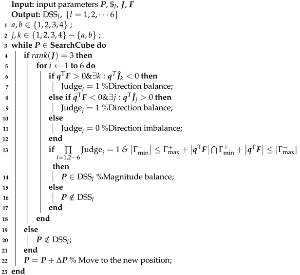
Since there are six possibilities for selecting two column vectors randomly from four column vectors of the Jacobian matrix J , the inner for-loop of Algorithm 2 will execute six times. The search space refers to SearchCube, which is a cube. After every inner for-loop, the position should move to the new position P + Δ P . Consequently, the algorithm of generating the subspace of DFFW can be summarized as Algorithm 2.
For a selected velocity–acceleration pair $ l ( l = 1 , 2 , 6 ) , a subspace of DFFW referred to as DSS l will be generated through implementing Algorithm 2 correspondingly. By repeatedly performing Algorithm 2 six times and taking the intersection of the subspaces DSS l , the DFFW DS will be generated. Mathematically, the relationship between DSS l and DS can be described as follows:
$ l DSS l DS DS = l = 1 , 2 , 6 DSS l
Algorithm 2: Generate the subspace of DFFW.
Machines 10 00565 i002

5. Optimization Model Establishment

5.1. Optimization Variables

The pulleys of the camera robot can be easily mounted on top of masts or the surface of buildings according to the characteristics of the shooting place, whose positions have a strong influence on the workspace, kinematics and dynamics. Therefore, it is reasonable to employ the positions of the pulleys as the optimization variables for structural optimization. Since the horizontal projection of the four pulleys on the ground is a rectangle, the global frame { o x y z } can be established with the origin fixed on the projection point of the #1 pulley. As Figure 7 displayed, we can use three dimensional parameters to describe the positions of four pulleys in { o x y z } , i.e., the length of the rectangle l e n , width of the rectangle w i d and the pulley height h e i . Thus, the position of #1 pulley is B 1 = 0 , 0 , h e i T , #2 pulley B 2 = l e n , 0 , h e i T , #3 pulley B 3 = l e n , w i d , h e i T and #4 pulley B 4 = 0 , w i d , h e i T .
In addition to the positions of the pulleys, the mass of the CPTDS also can be adjusted. Underweight or overweight CPTDS may affect the performance of the camera robot. Thus, the performance of the camera robot can be improved by choosing a suitable mass of the CPTDS. Hence, it is necessary to use the mass of the CPTDS m p as the optimization variables for structural optimization.
The optimization variables of structural optimization of the camera robot can be written in the following vector form:
D = l e n , w i d , h e i , m p T = [ d 1 , d 2 , d 3 , d 4 ] T ,
and the physical significance and unit of each optimization variable are shown in Table 1.

5.2. Optimization Objects

The camera robot is a high-speed and high-maneuverable manipulator, which will bring great challenges to take real-time video pictures. In order to find the video images with a sufficient scope and high-resolution ratio, a sufficiently large workspace and a stable enough camera are needed. In this paper, we attempt to enlarge the workspace and enhance the shooting stability through the structural optimization.

5.2.1. Workspace Volume

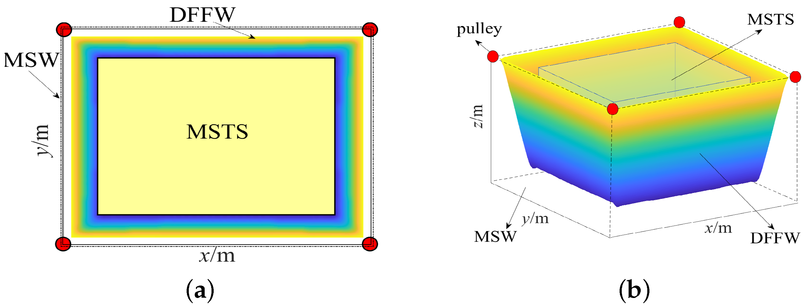
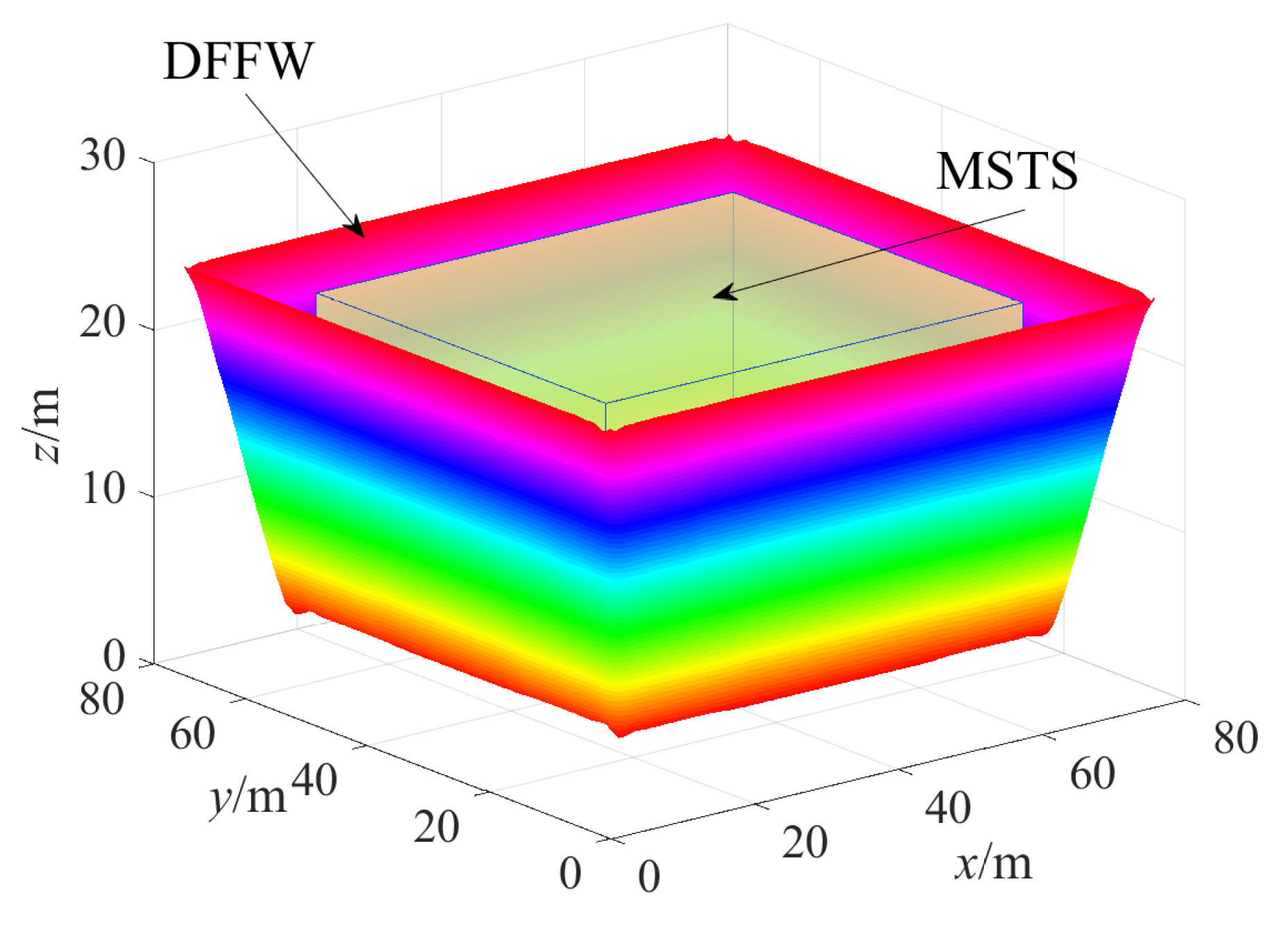
In order to satisfy the shooting requirements, it is desired to enable the camera robot to achieve as high ability of tracking photography as possible. The volume of the workspace is directly related to the tracking photography ability of the camera robot. The larger the workspace, the more areas the camera robot can capture. Naturally, the workspace volume can be integrated into the optimization model of the camera robot as the optimization object. Given the large-span and high-speed characteristics of the camera robot, the DFFW presented in the previous section is employed in this paper. As shown in Figure 8a, the rectangle determined by four pulleys forms the upper surface of the cube, which is the theoretical maximum workspace, referred to as the maximum shooting workspace (MSW). However, the shape of the actual workspace (DFFW) is similar to a reversed quadrilateral prism with a smaller bottom and a larger top as a result of restrictions on the tensions in cables.
As illustrated in Figure 8b, the horizontal section of the DFFW is a rectangle, which is analogous to the rectangle formed by four pulleys. In order to guarantee the shooting effect, a cube named the minimum shooting task-space (MSTS) is defined within MSW and is required to be included within the DFFW.
In this paper, we discretize the MSW, yielding the total number of point within the MSW N t o t a l . Then, we scan the every point within the MSW and record the number of points meeting the dynamic force-feasible condition N D F F W described in Equations (19) and (20). Finally, the volume of DFFW v o l can be obtained by computing the ratio of N D F F W to N t o t a l . The larger volume of DFFW, the stronger the ability of the tracking photography. Thus, the optimization objective for the workspace volume is as follows:
f 1 ( D ) = max v o l d 1 , d 2 , d 3 , d 4

5.2.2. Anti-Wind Disturbance Ability

Camera robots often function in high-rise cable support structures, which are inevitably disturbed by wind due to the frequent outdoor operations. Thus, enhancing the ability of anti-wind disturbance is crucial for maintaining the stability of the camera when taking videos and pictures. There are two kinds of wind forces acting on buildings, i.e., steady wind pressure and fluctuating wind pressure [46]. Since the period of the stable wind pressure is much larger than the natural vibration period of the general structure, its force can be regarded as a static force [47]. However, the high-frequency pulsation components of the fluctuating wind pressure lead to vibration responses of the camera robot, which have an influence on the camera robot’s normal operations.
The frequency characteristics of fluctuating wind can be expressed by its power spectrum, which is related to the surface roughness and geomorphic conditions. Considering that the camera robot mainly works in the open areas of urban spaces, the correction coefficient to the basic wind pressure w 0 is caused by the surface roughness μ w 0 = 0.731 . Given the air density ρ a = 1.225 kg / m 3 and the basic wind pressure w 0 = 0.35 KN / m 2 , the maximum 10-minute average wind speed V ¯ max with a 30-year return period can be calculated as follows [47]:
V ¯ max = 2 μ w 0 k 0 w 0 ρ a
where k 0 is the return period coefficient and k 0 = 1 is when the return period is 30 years. Since the frequently used Davenport spectrum overestimates the turbulence energy at high frequencies, these frequencies are of great significance for flexible tall structures. Therefore, this paper employs the modified Davenport wind speed spectrum—namely, the Maier spectrum, which can be written as follows [47]:
S v ( z , f ) = 2 x 2 ( 1 + 3 x 2 ) 4 3 · σ V 2 f x = L v * f V ¯ ( z ) σ V = 6 k V ¯ 10 V ¯ z = V ¯ 10 z 10 α
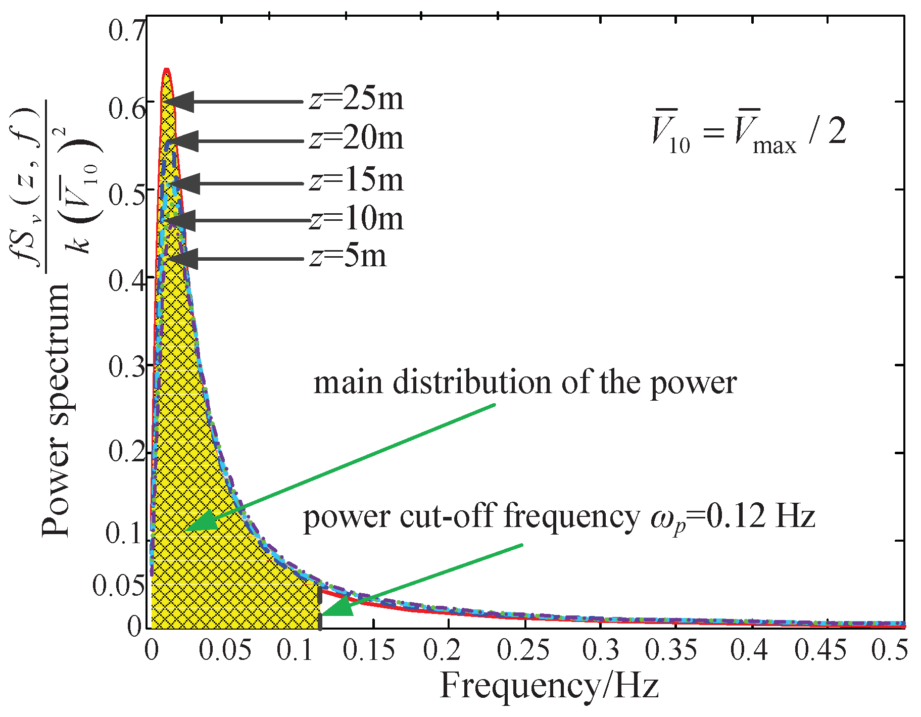
where z is the height of the CPTDS above the ground, L v * = 1200 m is the overall scale of the turbulence, and V ¯ 10 is average wind speed at 10 m. As the camera robot works under the common wind speed, the power spectrum of fluctuating wind can be obtained, which is shown in Figure 9.
On the one hand, as the height z changes from 5 to 25 m (the main working range of the camera robot), the power spectrum varies accordingly. It can be seen from Figure 10 that the maximal value of the power spectrum increases with the increasing pulley height. However, the values of five curves mainly exist in the range of 0.01–0.12 Hz, which is also the most-concentrated region of the energy of the pulsating wind. The maximum values of the five power spectrum curves both emerge at 0.02 Hz and then fall quickly; when the frequency is more than 0.12 Hz, the power spectrum is less than 0.05. Hence, we define 0.12 Hz as the energy cut-off frequency. In the study of anti-wind disturbance, we focused on the energy concentrated region, i.e., the frequency region of the pulsating wind between 0.01 and 0.12 Hz. On the other hand, we obtained the minimum first-order natural frequencies on the horizontal sections of the dynamic feasible workspace at different heights. As shown in Figure 10, the minimum first-order nature frequency is 0.13 Hz when z = 10 m. Therefore, the CPTDS will produce a vibration as the result of the wind-excitation at certain areas within the workspace (such as the workspace boundaries). Therefore, in order to improve the ability of the camera robot to resist wind disturbance, it is necessary to increase its first-order natural frequency to keep away from the range of 0.01–0.12 Hz.
The transverse and longitudinal vibrations of the cable may occur in the vertical plane when the cable is disturbed by the wind. For the cable, the influence of longitudinal vibration on the end-effector is much greater than that of transverse vibration. Diao et al. indicated that the influence of transverse vibration on the end-effector is only 1.4%, while that of longitudinal vibration on the end-effector is 98.4% [48]. Liu et al. suggested that the longitudinal vibration of the cable has a greater influence on the feed cabin supported in parallel by six cables [49]. As seen in Figure 9 and Figure 10, the lower the frequency of the camera robot, the more likely the camera robot was excited. As the first-order vibration has the most important effects in structural response, it is necessary to calculate the first-order natural frequency of the camera robot in the following form:
ω i = 1 eig J + T M J + diag S 1 , S 2 , S 3 , S 4 / E A i = 1 , 2 , 3
where J + is the Moore–Penrose generalized inverse of the Jacobin matrix J . eig is an eigenfunction to solve the eigenvalues. For the camera robot, there are three eigenvalues as the result of its three translational DOF. diag S 1 , S 2 , S 3 , S 4 = S 1 0 0 0 0 S 2 0 0 0 0 S 3 0 0 0 0 S 4 is a diagonal matrix. E and A are the elastic modulus and cross-section area of the cable separately. The first-order natural frequency ω 1 is the minimum of Equation (24):
ω 1 = min ω i
GFNF = 1 N t o t a l i = 1 N t o t a l ω 1 D
The GFNF should be as large as possible to improve the ability to resist the wind disturbance of the camera robot in the whole workspace. Therefore, the optimization objective of anti-wind disturbance performance is as follows:
f 2 ( D ) = max 1 N t o t a l i = 1 N t o t a l ω 1 d 1 , d 2 , d 3 , d 4

5.2.3. Impulse of Tensions on CPTDS

When the camera robot works normally, the cables remain tight, and hence the cable tension will exert a tractive force on the CPTDS. Due to the high maneuverable, the tension changes quickly in a tiny period of time, causing an impulse on the CPTDS exerted by the cables, which will clearly have a great influence on the camera robot, such as vibration of the camera or blurred shooting video pictures. The impact should be reduced as much as possible to ensure the normal operation of the camera robot. If the external force applied on the CPTDS and locus of the CPTDS are known, the equivalent force F e q of the tensions in the four cables can be computed according to Algorithm 1.
F e q = i = 1 4 t i
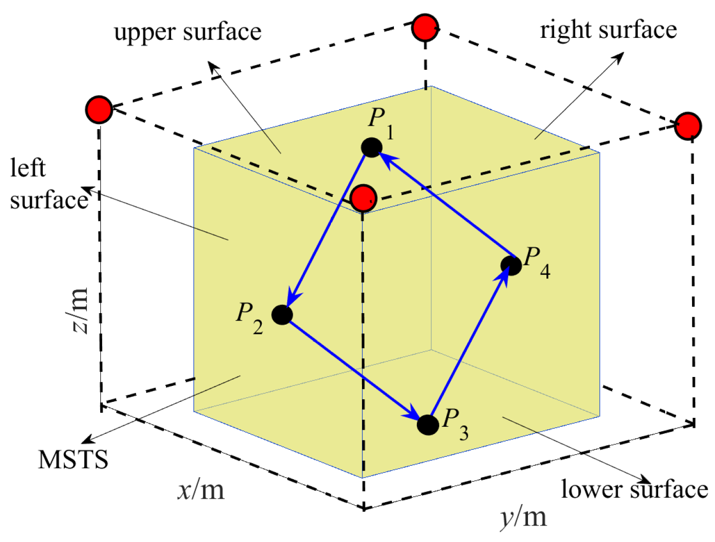
As shown in Figure 11, four sampling points, P 1 , P 2 , P 3 and P 4 , were selected. P 1 , P 2 , P 3 and P 4 are located in the upper, left, lower and right surfaces of the MSTS, respectively. Thus, the sampling locus of the cable tension impact function is P 1 P 2 P 3 P 4 P 1 . As the four sampling points are evenly distributed in MSTS and the acceleration varies dramatically at the points that the direction of locus changes, the impulse of tensions on the CPTDS will be great. Therefore, the selection of such a sampling locus can truly reflect the impact of the tensions on the CPTDS. The sum of impulse i m p along the sampling locus can be calculated by computing the impulse at every time point, which can be used as the evaluating function of impulse of tensions on the CPTDS.
i m p = 0 T F e q d t 2
where T is duration of the locus. In order to ensure that the impulse of CPTDS is as slight as possible, the impulse sum i m p should be kept as small as possible:
f 3 ( D ) = min i m p d 1 , d 2 , d 3 , d 4

5.3. Constraints

5.3.1. Linear Constraints

Considering the installation and site conditions, the optimization variable vector D should meet the following linear constraints to ensure that the camera robot has feasibility of structure.
lb D ub
where lb = [ l b 1 l b 2 l b 3 l b 4 ] T is the lower bound; ub = [ u b 1 u b 2 u b 3 u b 4 ] T is the upper bound.

5.3.2. Nonlinear Constraints

As described in the previous sections, the horizontal components of tensions have upper bound h max and lower bound h min . Furthermore, in order to ensure that the CPTDS has sufficient tracking and shooting abilities in the workspace, the workspace volume v o l ( D ) determined by the optimization variable vector D must be larger than the volume of MSTS Ω . To ensure that the camera robot has a strong ability of anti-wind disturbance, it is necessary to guarantee that the GFNF determined by D must be larger than the energy cut-off frequency ω p = 0.12 Hz. To sum up, the nonlinear constraints of camera robot structural optimization can be summarized as follows:
g 1 D = h min D h max 0 g 2 D = h max D + h min 0 g 3 D = V D + Ω 0 g 4 D = ω D + ω p 0
where h min and h max are the minimum and maximum values of the horizontal components of tensions with regard to the optimization variable vector D , respectively.

6. GA-Based Structural Optimization

6.1. Information Entropy-Based Adaptive Multi-Island GA

Structure optimization of a camera robot is intrinsically a highly nonlinear optimization problem. Moreover, it is difficult to obtain a continuous and derivable analytical expression of the workspace of the camera robot. Therefore, it is difficult to deal with this problem for the traditional optimization methods. However, SGA is subject to premature convergence, thereby, falling into local minimum easily. GA is an intelligent optimization method that simulates the evolution of organisms in nature and genetic laws. It was first proposed by Professor Holland in 1975 in the book Adaptation in Natural and Artistic Systems.
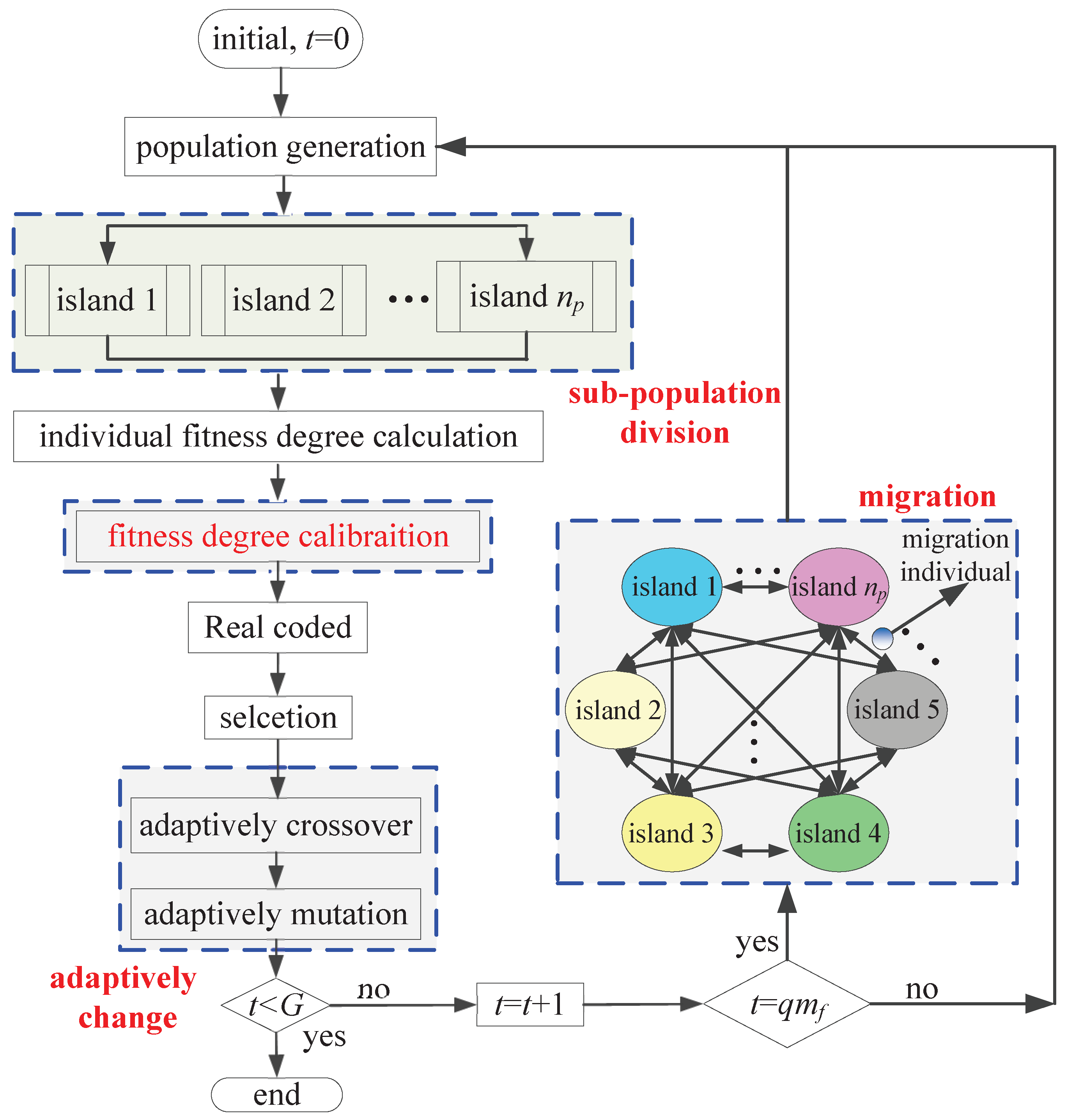
Multi-island GA divides each population into several sub populations—named islands—which can be viewed as a niche. As only the excellent individuals migrate between the islands, it can mean that excellent individuals spread to the whole population and improve the evolution level of the whole population [50]. In this paper, we propose a improved genetic algorithm incorporating into three improvements, namely fitness calibration, sub-population division and adaptive changes of crossover probability and mutation probability.

6.1.1. Fitness Degree Calibration

There may be special individuals with abnormal fitness in the initial population, leading to the dominance of the whole population possibly. At the end of the genetic process, the fitness of individuals tends to be consistent and the solution will swing around the optimal solution so that the optimal solution can not be searched. The selection ability of the population can be improved through enlarging fitness degree appropriately, which is the principle of fitness degree calibration and can be expressed as follows:
f i t ˜ = f i t 0 + f i t min f i t min + f i t max + δ
where f i t 0 is the original fitness degree; f i t min and f i t max are the lower and upper bound of fitness degree, respectively; and δ 0 , 1 is a positive real number to avoid the zero denominator. The purpose of f i t min is to guarantee the fitness degree is always positive after calibration.

6.1.2. Sub-Population Division

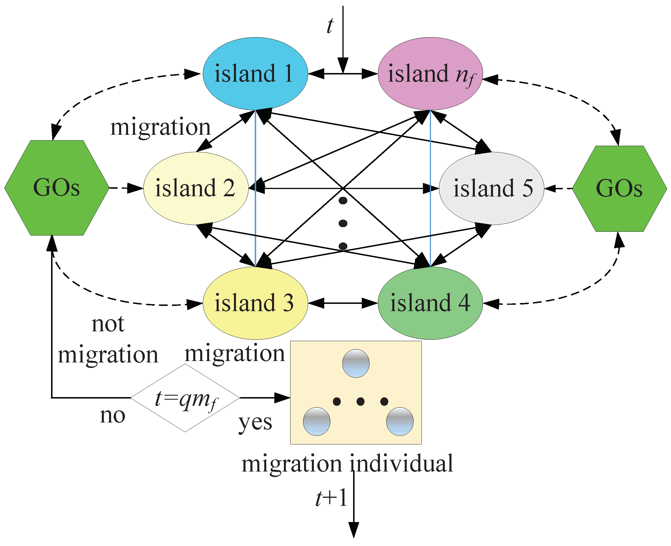
The mechanism of sub-population division and migration arises from the idea of multi-island GA, whose group is divided into several sub-populations referred to as islands. The selection, crossover and mutation operations of GA are performed on each island, and the migration operation is performed between different islands periodically. The steps of multi-island GA are shown in Figure 12, where t is the current generation, n f is the number of sub-population, q is positive integer, and m f is the migration interval.
GOs represents a genetic operation, such as selection, crossover, or mutation. Only when the number of generations reaches the integral multiple of the migration interval m f , will the individuals be transferred according to the migration rate i f between the islands; otherwise, the migrations will not occur but instead GOs. Through the sub-population division and migration, the diversity of solution to GA is improved to thus improve the ability to search the global optimal solution [51].

6.1.3. Adaptive Changes of Crossover Probability and Mutation Probability

When GA evolves to a certain generation, the fitness of the population will converge, and the population diversity will decline, allowing the algorithm to easily fall into the local optimal solution. In this paper, we regulate the crossover probability p c and mutation probability p m adaptively based on the information entropy of the population. Information entropy is a concept proposed by Shannon indicating the disorder degree of the system [52]. At the early stage of evolution, the diversity of the population and the disorder degree is high, and thus the information entropy is high. As the evolution process of the superior winning and the bad eliminated, the disorder degree of the population decreases, and then the information entropy decreases, which conforms to the law of biological development. The information entropy of the population can be defined as follows:
I t = i = 1 n p p t i log 2 p t i p t i = f i t t i i = 1 n p f i t t i
where n P is the total number of individuals in the population, and f i t t i is the fitness degree of the ith individual in the population of the tth generation. Thus, the adaptive operators of crossover rate P c t and mutation P m t rate of the population of the tth generation are as follows:
P c ( t ) = 1 + e I ( t ) / e I max 2 P c 0
P m ( t ) = 1 + e I ( t ) / e I max 2 P m 0
I max is the maximum information entropy and I max = log 2 n p . P c 0 and P m 0 are the initial values of crossover rate and mutation rate. According to GA theory, crossover rate ranges from 0.4 to 0.9, and the mutation rate ranges from 0.01 to 0.1 [51]. Therefore, P c 0 and P m 0 should be calculated several times according to the value range to obtain the appropriate value.

6.1.4. Population Information Entropy-Based Adaptive Multi-Island GA

Based on the three improvements, we propose an improved GA, i.e., the population information entropy-based adaptive multi-island Genetic Algorithm (PIEAMIGA) as illustrated in Figure 13. Compared to the standard genetic algorithm (SGA), PIEAMIGA adds three modules, namely sub-groups division, fitness calibration and migration, whose crossover rate and mutation rate vary according to the information entropy of the population. The optimization variable vector D = d 1 , d 2 , d 3 , d 4 T is the chromosome of PIEAMIGA that is coded by real values, and the selection is based on stochastic universal sampling. The entire process will stop when t = G , and the current optimization parameters will be exported; otherwise, it will re-generate a population and proceed to the next iteration.

6.2. Multi-Objective Structural Optimization

The main method to deal with the multi-objective structural optimization problem of CDPM is the weighted coefficient method [33,53,54]. However, the weighted coefficient method has three shortcomings: first, the weight coefficients are determined according to the designer’s subjective intention; second, the weight coefficients are difficult to quantify accurately; third, a single weight coefficient is difficult to represent all design intents due to the infinite selections of weight coefficients. In addition to the weighted coefficient method, there are some other multi-objective structural optimization methods for CDPMs, such as the enumeration method [55] and tabular method [56]. However, these methods are not objective, because the optimal criteria are determined by designers subjectively. Accordingly, we apply the ideal-point method to tackle the multi-objective structural optimization problem.
Process of the ideal-point method: first, three optimization objectives are conducted to obtain the optimal solution with regard to each objective; secondly, the solution spaces of the three objectives are normalized to the interval [0, 1], and the optimal value of each objective is normalized to “0”; finally, the minimum sum of the distances between the three optimization objectives and “0” is taken as the optimization objective, namely the “ideal point”. The PIEAMIGA was implemented with MATLAB programming language and executed on a notebook computer with a 2.2 GHz Intel Core I5-5200U CPU and a 12 G RAM.

6.2.1. The Optimal Value and Worst Value of Single-Objective Optimization

Since the GA itself does not have the ability to deal with constraints, it is necessary to transform the constrained optimization problem into unconstrained optimization problem, which can be realized through the penalty function method. Thus, the fitness function of the optimization object f i D with regard to design variable vector D is as follows:
F ˜ i ( D ) = f i t { sgn i T r a f i ( D ) + P u n j = 1 4 g j D j + g j D }
where f i t is the fitness degree function, and { i = 1 , 2 , 3 } . T r a is a transfer function. P u n is a large positive number and is used as the penalty factor.
The parameters of SGA and PIEAMIGA are listed in Table 2. The simulation parameters of the optimization model are shown in Table 3. According to the site and installation conditions, the range of the length l e n and width w i d of the horizontal projection rectangle of pulleys are [80, 90] m and [70, 80] m, respectively; the range of the height of the pulleys’ points is [25, 30] m. The range of the mass of the CPTDS is [20, 50] kg. The MSTS is a 70 m × 60 m × 22 m cuboid, whose volume Ω is 92,400 m 3 . Based on the parameters listed in Table 2 and Table 3, PIEAMIGA and SGA are programmed by MATLAB to find the optimal solution and value with regard to three optimization objects separately, which are listed in Table 4. The worst values with regard to the single optimization object are also listed in Table 4.
It can be seen from Table 4 that the optimal solution obtained by PIEAMIGA is better than that obtained by SGA. Workspace volume increases by 8.52%, the first-order natural frequency increases by 9.73%, and the impulse exerted by tensions on the CPTDS to CPTDS is reduced by 10.08%. Although three modules are added into PIEAMIGA based on SGA, the computing time of PIEAMIGA increases by 4.48% compared with that of SGA because the multi-island GA adopts the parallel mechanism, and operations in each island are performed in parallel. It also can be seen from Table 4 that PIEAMIGA has a stronger global search ability as the result of the adaptive crossover and mutation rate.
The convergence processes of each objective by the PIEAMIGA and SGA are shown in Figure 14. In the early stage of evaluation, the optimal solution changes rapidly due to the randomness of population and great differences between individuals, which is a sharply changed line in Figure 14a. With the progress of evolution, the number of excellent individuals in the population gradually increases; thus, the change of optimal solution slows down, and the local convergence appears, which is a horizontal line in Figure 14. Furthermore, the process of local convergence is prolonged gradually as the result of the increasing proportion of excellent individuals in the population.
Thus, the change of the optimal solution is not as violent as in the initial stage, and the length of the horizontal line is gradually longer with the increase in generation of evolution. There exist a jump after the local convergence process on the curve because the optimal solution jumps out of a local optimal solution and evolves towards a better optimal solution. It is inevitable that the performance of the offspring will be degraded compared with the parent because the new individuals are not always better than the parent individuals, which is a fluctuating line in Figure 14a. It can also be seen from Figure 14 that PIEAMIGA shows the better “climbing” (downhill) ability with the progress of evolution, and thus the gap between the two curves becomes increasingly larger. Finally, PIEAMIGA converges to the global optimal solution while SGA can only converge to the sub-optimal solution.
Figure 15a shows that the workspace boundary extends outwards after using PIEAMIGA and that the volume increases by 14,425 m 3 compared to SGA. Figure 15b shows that the first-order natural frequency on the horizontal section of workspace that the height z is 6 m has significantly increased after using PIEAMIGA, and the GFNF is increased by 0.0452 Hz compared to SGA. Figure 15c shows that the impulse sum to the CPTDS has decreased significantly after using PIEAMIGA, and the impulse sum is decreased by 2792 N·s compared to SGA.

6.2.2. Multi-Objective Optimization Based on the Ideal Point Approach

In the previous sections, we performed structural optimization with regard to the three optimization objectives, respectively. However, we want to optimize the three optimization objectives simultaneously, i.e., the largest workspace, the highest first-order nature frequency and the smallest impulse on CPTDS exerted by tensions. Mathematically, it is a multi-objective optimization problem and will be solved by using the ideal-point method.
Since the physical meaning of the three optimization objectives is different, it is necessary to normalize the three optimization objectives f 1 D , f 2 D and f 3 D , respectively. Thus, the three optimization objects become continuous functions in the [0,1] interval, and the multi-objective function is uniform in dimension. The maximum and minimum values of each optimization objective need to be normalized.
As shown in Table 4, for f 1 D , f 1 , min = f 1 = 84 , 875 m 3 , f 1 , max = f 1 * = 183 , 750   m 3 ; for f 2 D , f 2 , min = f 2 = 0.1042 Hz, f 2 , max = f 2 * = 0.3100 Hz; for f 3 D , f 3 , min = f 3 * = 24 , 907 N·s, f 3 , max = f 3 = 63 , 207 N·s. Thus, we can find three objectives after normalization:
f ¯ 1 D = f 1 , max f 1 ( D ) f 1 , max f 1 , min f ¯ 2 D = f 2 , max f 2 ( D ) f 2 , max f 2 , min f ¯ 3 D = f 3 ( D ) f 3 , min f 3 , max f 3 , min
According to the definition of the ideal-point method, the minimum sum of the distances between the three objective function and the three ideal points is taken as the optimization objective, and the linear and nonlinear constraints proposed in previous are taken as the optimization constraints:
min W ( D ) = i = 1 3 f ¯ i D s . t . L D U g 1 D = H min D h max 0 g 2 D = H max D + h min 0 g 3 D = V D + Ω 0 g 4 D = ω D + ω p 0

6.3. Results and Discussion of Multi-Objective Structural Optimization

According to the simulation parameters listed in Table 3 and Table 4, the multi-objective structural optimization is conducted by real-coded PIEAMIGA in the MATLAB environment. The results are listed in Table 5. It can be seen that the three optimization results are balanced, none of which is dominant, while others perform poorly.
Figure 16 shows the DFFW corresponding to the optimal solution D * , which completely contains the MSTS, and thus the filming work can be successfully completed.
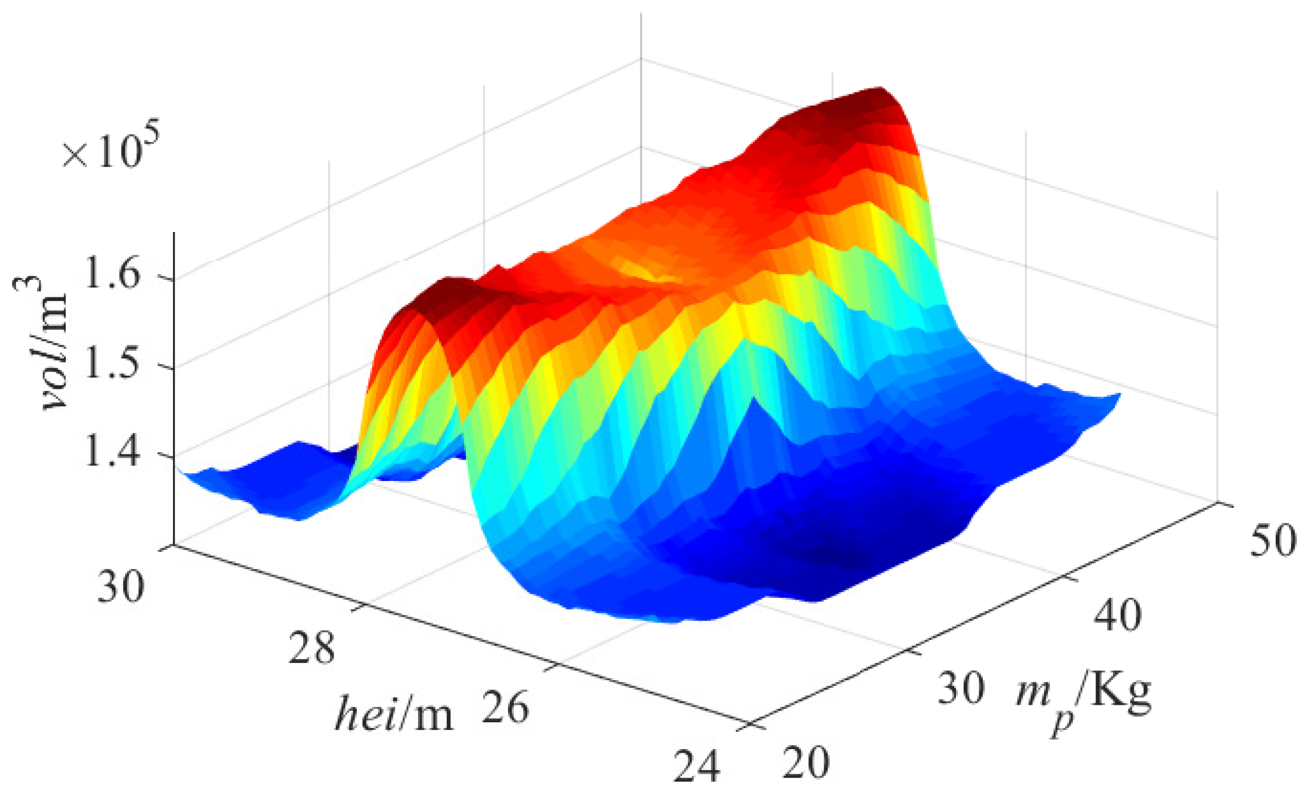
Figure 17 and Table 6 illustrate the relationship of the workspace volume v o l with the pulley point height h e i and the mass of CPTDS m p when the optimization variables d 1 and d 2 are fixed. In this case, l e n = d 1 * and w i d = d 2 * . The pulley height h e i is not positively correlated with volume of workspace v o l . It can be known from the curved surface that the volume is small at both ends and large in the middle. It can be seen from Table 6 that the workspace volumes are about the same when the pulley height is equal to 27 and 28 m, and thus the maximum value is near h e i = 27.5 m.
Generally speaking, the higher the pulley height h e i is, the larger the volume is. However, the tension range is also a decisive factor of workspace. With the increase in height h e i , the angle between the tangent line at the cable end and the direction of gravity decreases; thus, the cable tension must be increased to balance the gravity. The increase in height h e i will cause an increase in the length and weight of the cable, and thus an increase in the cable tension. Thus, it is possible that the tensions exceed the upper limit h max , leading to a decrease in the workspace that is mainly located in the area near the pulley point close to the upper surface of the workspace.
Relatively speaking, the relationship between the mass of CPTDS and the workspace volume is obvious, which has two characteristics: (1) Positive correlation. The light mass of CPTDS may give rise to the decrease in cable tension, or even less than the lower limit h min . The reduced volume of workspace is mainly located at the boundaries of the workspace, where the area of the cable tension is relatively small. (2) At the beginning of the curve, the increase is obvious; however, at the end of the curve, the change is small.
When the mass m p is small, increasing the mass of CPTDS will significantly enhance the cable tension so that many position points that originally do not meet the lower limit h min satisfy the lower limit h min again. Therefore, the volume of workspace increases. However, when the mass m p increases to a certain extent, the minimum tension at most of the m p points have been greater than h min . Therefore, the increase in the workspace volume v o l is limited.
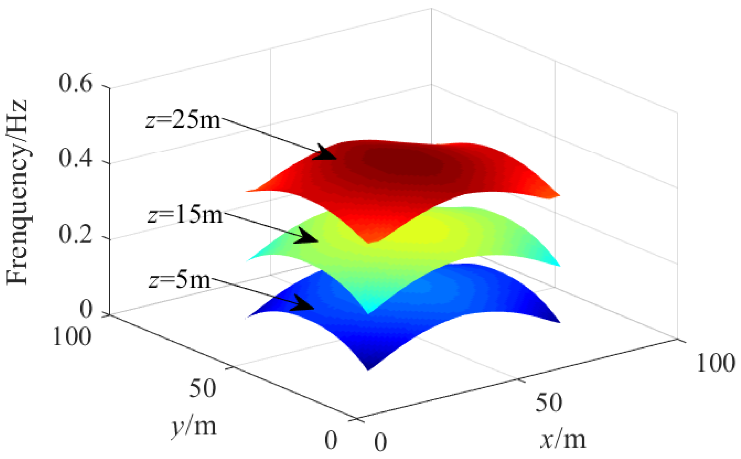
Figure 18 shows the spatial distribution of the first-order natural frequency corresponding to the “ideal point” on three horizontal sections of the workspaces at different heights, i.e., z = 5 m, z = 15 m and z = 25 m. Clearly, the higher the height along the z axis is, the higher the natural frequency is. Since the camera robot belongs to the suspended CDPM, the four pulley points are all above the CPTDS. Therefore, the higher the height along z axis is, the shorter the cable length is. According to Equation (25), the shorter the cable length, the higher the natural frequency of the camera robot. Similarly, there is always a long cable when the CPTDS at one of the four corners of the workspace; hence, the first-order natural frequency of the camera robot will be smaller, leading to a downward sharp corner.
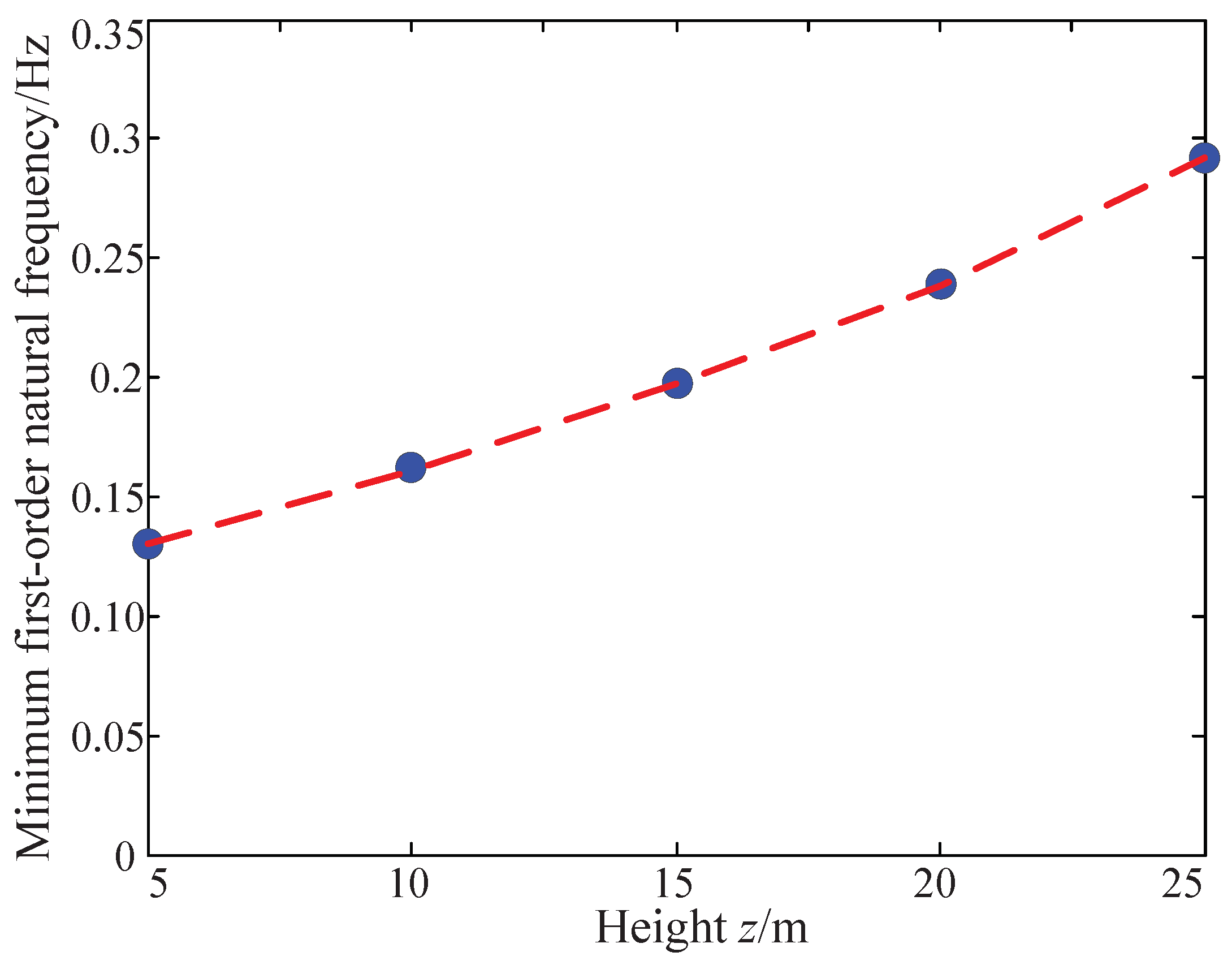
Figure 19 shows the minimum value of the first-order natural frequency on the different horizontal sections of the workspace with different heights, which are significantly improved compared with those shown in Figure 10. The minimum first-order natural frequency on each horizontal section all exceeds 0.12 Hz. At z = 5 m, the minimum first-order natural frequency is equal to 0.13 Hz. Although it has been improved, it is still close to the energy truncation frequency ω p = 0.12 Hz. Therefore, it is still vulnerable to wind disturbance. Thus, some measures are essential to enhance the first-order natural frequency of the camera robot, such as the stiffness improvement and tension regulation.
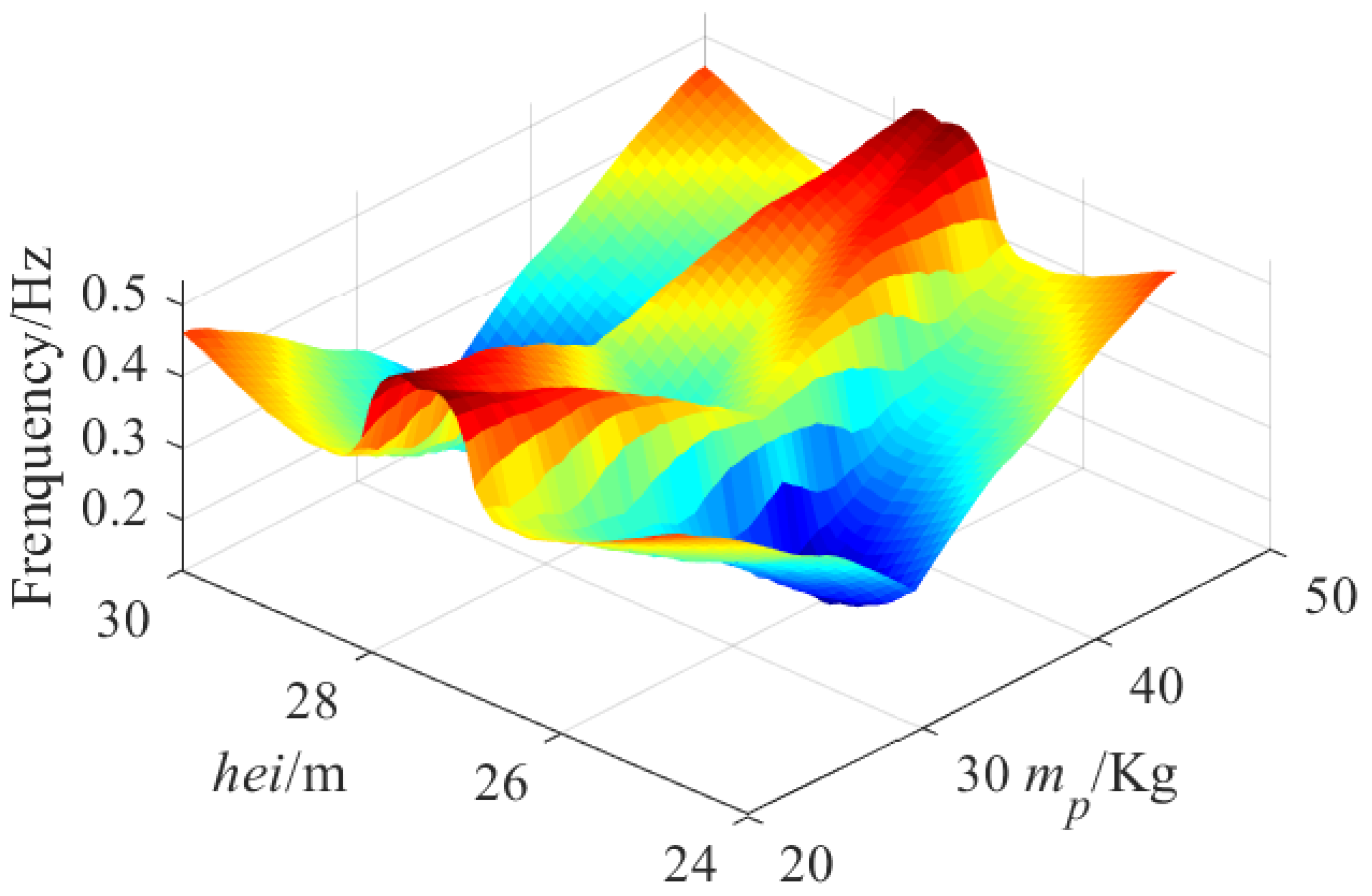
Figure 20 and Table 7 show the relationship of GFNF with the pulley point height h e i and the mass of CPTDS m P when the optimization variables d 1 and d 2 are fixed. In this case, l e n = d 1 * and w i d = d 2 * . The relationship between GFNF and h e i is not proportional, but exhibits the characteristics of “high at both ends, low in the middle”. It can be concluded from Equation (21) that the critical factor of determining the GFNF is the length of the cable. On the one hand, the smaller the height h e i is, the smaller the length of the cable is. Thus, the frequency is larger when h e i = 25 m; However, on the other hand, the decrease in height h e i will lead to the decrease in the height of workspace, lead to losing some points in workspace.
Since the cable length at these “losing point” is shorter, the first-order natural frequency is larger. Therefore, the whole level of the natural frequency in the workspace will decrease after losing these points. Hence, the contradiction between them determines that the value of GFNF is larger when h e i is equal to the maximum or minimum height and smaller when h e i is in the middle height. The relationship between the mass of CPTDS m p and GFNF is very obvious. The greater the mass is, the lower the frequency is. We can observed that the GFNFs are the same when the pulley height at 27 m and 28 m. We can also draw the conclusion that the GFNF is more sensitive to the pulley height than the mass of the CPTDS.
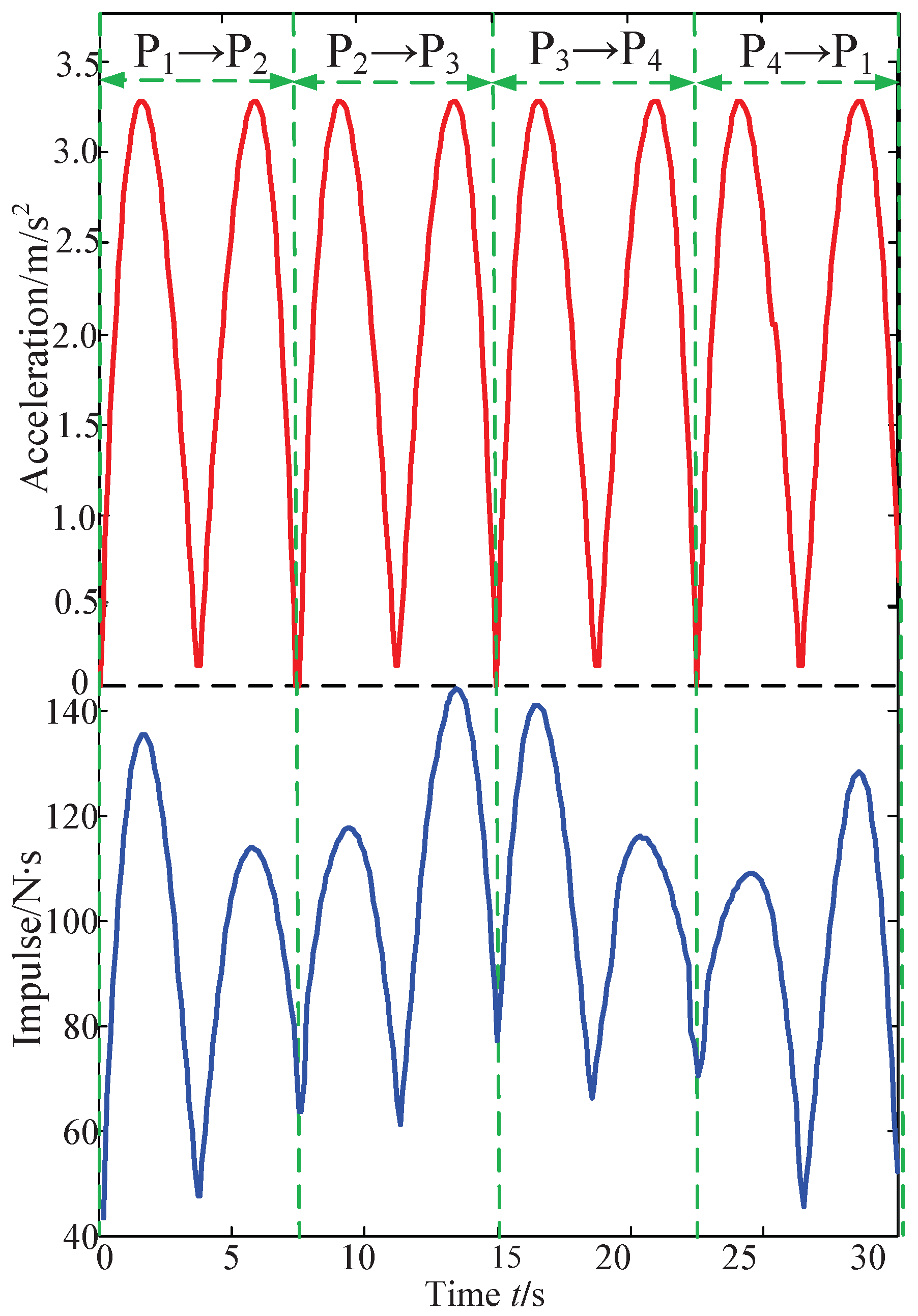
Figure 21 shows the impulse applied on the CPTDS and the accelerations of the CPTDS corresponding to the optimization solution following the sampling locus shown in Figure 11. Since every straight line segment of the locus is planned by a quintic polynomial, the acceleration curve is a cubic curve, and the value of acceleration at each point change motion direction of the locus is 0. It can be seen that the impulse is larger in the time point with larger acceleration, reflecting the tensions exert a large impulse on the CPTDS at this time point. The maximum value appears at t = 15 s, when the CPTDS moves near the point P 3 and is close to the lower surface of the workspace.
Therefore, the cable length and tension are larger than those at the rest points and thus the impulse. It can be observed that the curve is not completely symmetrical on both sides with P 3 as the center. However, the left side is larger and the right side is smaller. As the segment P 2 P 3 is on the left side of P 3 and the motion direction is consistent with the direction of gravity, the tension is larger; the motion direction of the segment P 3 P 4 on the right side of P 3 is contrary to the gravity direction, and therefore the tension is smaller. Thus, the impulse on the segment P 2 P 3 is larger than that on the segment P 3 P 4 . Similarly, the impulse applied on the CPTDS on the segment P 1 P 2 is larger than that on the segment P 4 P 1 .
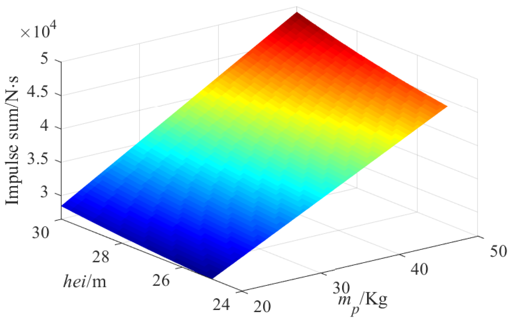
Figure 22 and Table 8 show the relationship of the impulse sum on the CPTDS along the sampling locus with the pulley point height h e i and the mass of CPTDS m p when the optimization variables d 1 and d 2 are fixed. In this case, l e n = d 1 * and w i d = d 2 * . There is a positive correlation of the impulse sum with the pulley point height h e i and the mass of CPTDS m p . The higher the pulley point height h e i and the greater the mass m p of the CPTDS are, the greater the impulse sum will be. In addition, it can be observed from Table 8 that the impulse sum linearly increases with increasing of the pulley point height and the mass of the CPTDS.
7. Conclusions

In this paper, the dynamic modeling of the camera robot was presented considering the self-weight and inertia of the cable simultaneously, which was also fit to other large-span and high-speed manipulators, and a tension distribution algorithm was developed based on the iteration method. According to the dynamical model, an approach of generating a dynamic feasible workspace was proposed. In order to improve the shooting ability of the camera robot, the structure of the camera was optimized by optimizing the three objectives separately and then mixed together using the ideal point method through a modified GA. Furthermore, the characteristics of the objectives were analyzed by varying the design parameters. The main contributions of this study include the following:
First, the dynamic model of the large-span high-speed camera robot with redundant actuation combining with the cable mass and inertia is established. Based on this model, an iterative-based tension distribution algorithm (Algorithm 1) was proposed to determine the tensions in cables given the position of the CPTDS. In addition, a dynamic force-feasible workspace (DFFW) generation algorithm (Algorithm 2) was proposed according to the characteristics of the camera robot based on the judging conditions of DFFW that contain the direction balance condition (DBC) and the magnitude balance condition (MBC) simultaneously. In this study, the three-DOF four-cable-driven camera robot was considered for illustrative case-studies. The presented algorithms were applicable to any cable-driven parallel manipulators while modifying the Jacobian matrix J , the generalized external force M , the unit normal vector q and the velocity–acceleration pair $.
Secondly, an optimization model of the camera robot was set up aiming to achieve the best workspace volume of DFFW, anti-wind disturbance ability and impulse exerted by tensions on CPTDS, where the anti-wind disturbance ability can be evaluated through the GFNF (global first-order nature frequency).
Thirdly, the multi-island and information entropy ideas were used to improve the SGA. Thus, an improved genetic algorithm was created in order to optimize the structure of the camera robot, namely the population information entropy-based adaptive genetic algorithm (PIEAMIGA). It can be seen from Figure 14 and Figure 15 that PIEAMIGA offered the stronger global search capability and the better optimization results compared with SGA with regard to each optimization objective while the computing time increased slightly as shown in Table 4.
Fourthly, the ideal-point method was employed to deal with the multi-objective structural optimization to avoid the influence of the subjective intention of the designer. The ideal point of each optimization objective was obtained by conducting single-objective structural optimization through PIEAMIGA. The optimization results with regard to the optimal solution D * by using PIEAMIGA are shown in Table 5 and demonstrate that the three optimization results were balanced. Figure 16, Figure 18, Figure 19 and Figure 21 illustrate the workspace shape, spatial distribution of first-order natural frequency, the minimum first-order natural frequency on different horizontal planes of workspace and the impulse on the CPTDS when the optimization variables are equal to the optimal solution D * .
Moreover, the relationship of the three optimization objectives with the pulley height h e i and the mass of CPTDS m p were studied as illustrated in Figure 17, Figure 20 and Figure 22 as well as Table 6, Table 7 and Table 8. Moreover, some laws were summarized, and these will be valuable for the design of camera robots. Furthermore, the design methodology presented in this paper can be extended to other classes of large-span high-speed CDPMs as well. Apart from the camera robot, the dynamic workspace generation approach and design methodology presented in this paper can be extended to other classes of large-span high-speed CDPMs as well. The next steps involve dynamic modeling for the complex spatial robot architectures and finally practical testing. Our future research will be focused on the motion control issue based on the dynamical model in this paper.

Author Contributions

Conceptualization, Y.S. and Y.Q.; methodology, Y.S.; software, P.L.; validation, Y.S. and P.L.; formal analysis, Y.Q.; investigation, P.L.; resources, Q.W.; data curation, X.W.; writing—original draft preparation, Y.S.; writing—review and editing, P.L.; supervision, Y.Q.; project administration, Y.S.; and funding acquisition, Y.S. and J.T. All authors have read and agreed to the published version of the manuscript.

Funding

This research was funded by Science and Technology Project of Shaanxi Province of China (Grant numbers: 2020JM-558, 2020GY-188 and 2015KTZDGY-02-01).

Institutional Review Board Statement

Not applicable.

Informed Consent Statement

Not applicable.

Data Availability Statement

Not applicable.

Conflicts of Interest

The authors declare no conflict of interest.

References

  1. Su, Y.; Qiu, Y.Y.; Sheng, Y. Optimal cable tension distribution of the high-speed redundant driven camera robots considering cable sag and inertia Effects. Adv. Mech. Eng. 2014, 2014, 729020. [Google Scholar] [CrossRef] [Green Version]
  2. Su, Y.; Qiu, Y.Y.; Liu, P. The continuity and real-time performance of the cable tension determining for a suspend cable-driven parallel camera robot. Adv. Robot. 2015, 29, 743–752. [Google Scholar] [CrossRef]
  3. Bai, G.; Ge, Y.; Scoby, D.; Leavitt, B.; Stoerger, V.; Kirchgessner, N.; Irmak, S.; Graef, G.; Schnable, J.; Awada, T. NU-Spidercam: A large-scale, cable-driven, integrated sensing and robotic system for advanced phenotyping, remote sensing, and agronomic research. Comput. Electron. Agric. 2019, 160, 71–81. [Google Scholar] [CrossRef]
  4. Yu, X.D.; Duan, L.; Tian, Q. Highway traffic information extraction from Skycam MPEG video. In Proceedings of the 2002 IEEE fifth International Conference on Intelligent Transportation Systems, Singapore, 3–6 September 2002; pp. 37–42. [Google Scholar] [CrossRef]
  5. Uva, M. The Grip Book, 4th ed.; Elsevier: Burlington, MA, USA, 2010; Chapter Cablecam; pp. 295–296. [Google Scholar] [CrossRef]
  6. Wei, H.L.; Qiu, Y.Y.; Sheng, Y. On the Cable Pseudo-Drag Problem of Cable-Driven Parallel Camera Robots at High Speeds. Robotica 2019, 37, 1695–1709. [Google Scholar] [CrossRef]
  7. Wei, H.L.; Qiu, Y.Y.; Sheng, Y. An approach to evaluate stability for cable-driven parallel camera robots with hybrid tension-stiffness properties. Int. J. Adv. Robot. Syst. 2015, 12, 1–12. [Google Scholar] [CrossRef] [Green Version]
  8. Liu, P.; Qiu, Y.Y.; Sheng, Y. A new hybrid force-position measure approach on the stability for a camera robot. J. Mech. Eng. Sci. 2016, 230, 2508–2516. [Google Scholar] [CrossRef]
  9. Ouyang, B.; Shang, W.W. Wrench-feasible workspace based optimization of the fixed and moving platforms for cable-driven parallel manipulators. Robot. Comput.-Integr. Manuf. 2014, 30, 629–635. [Google Scholar] [CrossRef]
  10. Fattah, A.; Agrawal, S.K. On the design of cable-suspended planar parallel robots. J. Mech. Des. 2005, 127, 1021–1028. [Google Scholar] [CrossRef]
  11. Zhang, Z.K.; Shao, Z.F.; Wang, L.P. Optimization and implementation of a high-speed 3-DOFs translational cable-driven parallel robot. Mech. Mach. Theory 2020, 145, 103693. [Google Scholar] [CrossRef]
  12. Hussein, H.; Santo, J.C.; Izard, J.B.; Gouttefarde, M. Smallest maximum cable tension determination for cable-driven parallel robots. IEEE Trans. Robot. 2021, 34, 1186–1205. [Google Scholar] [CrossRef]
  13. Hamed, J.; Khajepour, A.; Fidan, B.; Rushton, M. Kinematically-constrained redundant cable-driven parallel robots: Modeling, redundancy analysis, and stiffness optimization. IEEE/ASME Trans. Mechatron. 2017, 22, 921–930. [Google Scholar] [CrossRef]
  14. Anson, M.; Alamdari, A.; Venkat, K. Orientation workspace and stiffness optimization of cable-driven parallel manipulators with base mobility. J. Mech. Robot. 2017, 9, 031011. [Google Scholar] [CrossRef]
  15. Cui, Z.W.; Tang, X.Q.; Hou, S.H.; Sun, H.N.; Wang, D.J. Optimization design of redundant cable driven parallel robots based on constant stiffness space. In Proceedings of the 2019 IEEE International Conference on Robotics and Biomimetics (ROBIO), Dali, China, 6–8 December 2019; pp. 1041–1046. [Google Scholar] [CrossRef]
  16. Otis, M.J.; Perreault, S.; Nguyen-Dang, T.; Lambert, P.; Gouttefarde, M.; Laurendeau, D.; Gosselin, C. Determination and management of cable interferences between two 6-DOF foot platforms in a cable-driven locomotion interface. IEEE Trans. Syst. Man Cybern. Part A Syst. Humans 2009, 39, 528–544. [Google Scholar] [CrossRef]
  17. Otis, J.D.; Youssef, K. Reconfigurable fully constrained cable driven parallel mechanism for avoiding interference between cables. Mech. Mach. Theory 2020, 148, 103781. [Google Scholar] [CrossRef]
  18. Gallina, P.; Rosati, G. Manipulability of a planar wire driven haptic device. Mech. Mach. Theory 2002, 37, 215–228. [Google Scholar] [CrossRef]
  19. Gouttefarde, M.; Collard, J.F.; Nicolas, R.; Baradat, C. Geometry selection of a redundantly actuated cable-suspended parallel robot. IEEE Trans. Robot. 2017, 31, 501–510. [Google Scholar] [CrossRef] [Green Version]
  20. Li, Y.; Xu, Q. GA-based multi-objective optimal design of a planar 3-DOF cable-dDriven parallel manipulator. In Proceedings of the 2006 IEEE International Conference on Robotics and Biomimetics, Kunming, China, 17–20 December 2006; pp. 1360–1365. [Google Scholar] [CrossRef]
  21. Jamwal, P.K.; Xie, S.Q.; Aw, K.C. Multi criteria optimal design of cable driven ankle rehabilitation robot. In Mobile Robots-State of the Art in Land, Sea, Air, and Collaborative Missions; InTech: Rijeka, Croatia, 2009; Volume 1, Chapter 14; pp. 303–336. [Google Scholar] [CrossRef] [Green Version]
  22. Arsenault, M. Optimization of the prestress stable wrench closure workspace of planar parallel three-degree-of-freedom cable-driven mechanisms with four cables. In Proceedings of the 2010 IEEE International Conference on Robotics and Automation, Anchorage, AK, USA, 3–7 May 2010; pp. 1182–1187. [Google Scholar] [CrossRef]
  23. Bahrami, A.; Bahrami, M.N. Optimal design of a spatial four cable driven parallel manipulator. In Proceedings of the 2011 IEEE International Conference on Robotics and Biomimetics, Karon Beach, Thailand, 7–11 December 2011; pp. 2143–2149. [Google Scholar] [CrossRef]
  24. Amine, L.M.; Giuseppe, C.; Said, Z. On the optimal design of cable driven parallel robot with a prescribed workspace for upper limb rehabilitation tasks. J. Bionic Eng. 2019, 16, 503–513. [Google Scholar] [CrossRef]
  25. Hamida, I.B.; Laribi, M.A.; Mlika, A.; Romdhane, L.; Carbone, G. Multi-objective optimal design of a cable driven parallel robot for rehabilitation tasks. Mech. Mach. Theory 2021, 156, 104141. [Google Scholar] [CrossRef]
  26. Riehl, N.; Gouttefarde, M.; Krut, S.; Baradat, C.; Pierrot, F. Effects of non-negligible cable mass on the static behavior of large workspace cable-driven parallel mechanisms. In Proceedings of the 2011 IEEE International Conference on Robotics & Automation, Karon Beach, Thailand, 7–11 December 2011; pp. 2143–2149. [Google Scholar] [CrossRef]
  27. Dallej, T.; Gouttefarde, M.; Andreff, N.; Hervé, P.; Martinet, P. Modeling and vision-based control of large-dimension cable-driven parallel robots using a multiple-camera setup. Mechatronics 2019, 61, 20–36. [Google Scholar] [CrossRef] [Green Version]
  28. Gouttefarde, M.; Collard, J.; Riehl, N.; Baradat, C. Simplified static analysis of large-dimension parallel cable-driven robots. In Proceedings of the 2012 IEEE International Conference on Robotics and Automation, Saint Paul, MN, USA, 14–18 May 2012; pp. 2299–2305. [Google Scholar] [CrossRef]
  29. Nguyen, D.Q.; Gouttefarde, M.; Company, O.; Pierrot, F. On the simplifications of cable model in static analysis of large-dimension cable-driven parallel robots. In Proceedings of the 2013 IEEE/RSJ International Conference on Intelligent Robots and Systems, Tokyo, Japan, 3–7 November 2013; pp. 928–934. [Google Scholar] [CrossRef] [Green Version]
  30. Jiang, X.L.; Huang, Y.J.; Zheng, Y.Q. Dimension optimization design of an under-restrained 6-DOF four-cable-driven parallel manipulator based on least square-support vector regression. In Proceedings of the 2011 IEEE International Conference on Mechatronics and Automation, Beijing, China, 7–10 August 2011; pp. 458–463. [Google Scholar] [CrossRef]
  31. Yao, R.; Tang, X.; Wang, J.; Huang, P. Dimensional optimization design of the four-cable-driven parallel manipulator in FAST. IEEE/ASME Trans. Mechatron. 2010, 15, 932–941. [Google Scholar] [CrossRef]
  32. Tang, X.Q.; Yao, R. Dimensional design on the six-cable driven parallel manipulator of FAST. J. Mech. Des. 2011, 133, 111012. [Google Scholar] [CrossRef]
  33. Du, J.; Bao, H.; Cui, C. Stiffness and dexterous performances optimization of large workspace cable-driven parallel manipulators. Adv. Robot. 2014, 28, 187–196. [Google Scholar] [CrossRef]
  34. Wei, H.L.; Qiu, Y.Y.; Luo, L.F.; Lu, Q.H. An approach on stability analysis of cable-driven parallel robots considering cable mass. AIP Adv. 2021, 11, 055014. [Google Scholar] [CrossRef]
  35. Yu, L.L.; Qiu, Y.Y.; Su, Y. Dynamic workspace of a high-speed cable-driven camera robot. Eng. Mech. 2013, 30, 245–250. [Google Scholar]
  36. Barrette, G.; Gosselin, C.M. Determination of the dynamic workspace of cable-driven planar parallel mechanisms. J. Mech. Des. 2005, 127, 242–248. [Google Scholar] [CrossRef]
  37. Kawamura, S.; Kino, H.; Won, C. High-speed manipulation by using parallel wire-driven robots. Robotica 2000, 18, 13–21. [Google Scholar] [CrossRef]
  38. Lenarčič, J.; Merlet, J.P. (Eds.) Determination of a dynamic feasible workspace for cable-driven parallel robots. In Advances in Robot Kinematics 2016; Springer Nature: Cham, Switzerland, 2009; Volume 4, Chapter 35; pp. 361–370. [Google Scholar] [CrossRef] [Green Version]
  39. Kieu, V.N.D.; Huang, S.C. Dynamic and Wrench-Feasible Workspace Analysis of a Cable-Driven Parallel Robot Considering a Nonlinear Cable Tension Model. Appl. Sci. 2022, 12, 244. [Google Scholar] [CrossRef]
  40. Su, Y.; Qiu, Y.Y.; Wei, H.L. Dynamic modeling and tension optimal distribution of cable-driven parallel robots considering cable mass and inertia force effects. Eng. Mech. 2016, 33, 231–239. [Google Scholar] [CrossRef]
  41. Verhoeven, R. Analysis of the Workspace of Tendon-Based Stewart Platforms. Ph.D. Thesis, University of Duisburg-Essen, Duisburg, Germany, 2004. [Google Scholar]
  42. Irivne, H.M. Cable Structures, 1st ed.; The MIT Series in Structural Mechanics; MIT Press: Cambridge, MA, USA, 1981. [Google Scholar] [CrossRef]
  43. Diao, X.; Ou, M. A method of verifying force-closure condition for general cable manipulators with seven cables. Mech. Mach. Theory 2007, 42, 1563–1576. [Google Scholar] [CrossRef]
  44. Gouttefarde, M.; Daney, D.; Merlet, J.P. Interval-analysis-based determination of the wrench-feasible workspace of parallel cable-driven robots. IEEE Trans. Robot. 2011, 27, 1–13. [Google Scholar] [CrossRef] [Green Version]
  45. Liu, X.; Qiu, Y.Y.; Sheng, Y. Proofs of Existence Conditions for Workspaces of Wire-driven parallel robots and a uniform solution strategy for the workspaces. J. Mech. Eng. 2010, 46, 27–34. [Google Scholar] [CrossRef]
  46. Qiu, Y.Y.; Duan, B.Y.; Wei, Q.; Nan, R.D.; Peng, B. Optimal distribution of the cable tensions and structural vibration control of the cable-cabin flexible structure. Struct. Eng. Mech. 2002, 14, 39–56. [Google Scholar] [CrossRef]
  47. Qiu, Y.Y.; Chen, J.; Duan, B.Y. Simulation of the Wind Induced Vibration of the Suspended Feed Cabin in the largest Radio Telescope under random force. Chin. J. A Mech. 2000, 17, 91–95. [Google Scholar] [CrossRef]
  48. Diao, X.M.; Ma, O. Vibration analysis of cable-driven parallel manipulators. Multibody Syst. Dyn. 2009, 21, 347–360. [Google Scholar] [CrossRef]
  49. Liu, Z.H.; Tang, X.Q.; Shao, Z. Research on longitudinal vibration characteristic of the six-cable-driven parallel manipulator in FAST. Adv. Mech. Eng. 2013, 2013, 547416. [Google Scholar] [CrossRef] [Green Version]
  50. Zhang, W.; Qi, H.; Yu, Z.Q.; He, M.J.; Ren, Y.T.; Li, Y. Optimization configuration of selective solar absorber using multi-island genetic algorithm. Sol. Energy 2021, 224, 947–955. [Google Scholar] [CrossRef]
  51. Srinivas, M.; Patnaik, L.M. Adaptive probabilities of crossover and mutation in genetic algorithms. IEEE Trans. Syst. Man Cybern. 2002, 24, 656–667. [Google Scholar] [CrossRef] [Green Version]
  52. Shannon, C.E. A mathematical theory of communication. Bell Syst. Tech. J. 1948, 27, 379–423. [Google Scholar] [CrossRef] [Green Version]
  53. Khakpour, H.; Birglen, L.; Tahan, S.A. Analysis and optimization of a new differentially driven cable parallel robot. J. Mech. Robot. 2015, 7, 034503. [Google Scholar] [CrossRef] [Green Version]
  54. Sun, H.; Hou, S.; Li, Q.; Tang, X. Research on the configuration of cable-driven parallel robots for vibration suppression of spatial flexible structures. Aerosp. Sci. Technol. 2021, 109, 106434. [Google Scholar] [CrossRef]
  55. Abdolshah, S.; Zanotto, D.; Rosati, G.; Agrawal, S.K. Optimizing Stiffness and Dexterity of Planar Adaptive Cable-Driven Parallel Robots. J. Mech. Robot. 2017, 9, 031004. [Google Scholar] [CrossRef]
  56. Zhang, F.; Shang, W.; Zhang, B.; Cong, S. Design optimization of redundantly actuated cable-driven parallel robots for automated Warehouse System. IEEE Access 2020, 8, 56867–56879. [Google Scholar] [CrossRef]
Figure 1. Schematic of a camera robot configuration.
Machines 10 00565 g001
Figure 2. Catenary model of the cable in the vertical plane.
Machines 10 00565 g002
Figure 3. In-plane and out-plane motions of the cable.
Machines 10 00565 g003
Figure 4. Catenary model of the cable in a vertical plane.
Machines 10 00565 g004
Figure 5. Normal vector of the hyperplane and the generalized external force.
Machines 10 00565 g005
Figure 6. The projections of the tension and generalized external force in DBC and MBC. (a) The projections in DBC. (b) The projections in MBC.
Machines 10 00565 g006
Figure 7. Optimization variables of the camera robot.
Machines 10 00565 g007
Figure 8. The DFFW, MSTS and MSW of the camera robot. (a) Top view. (b) Main view.
Machines 10 00565 g008
Figure 9. Power spectrum of the pulsating wind (wind speed is the half of the maximum 30-year wind speed).
Machines 10 00565 g009
Figure 10. The minimum first-order natural frequency on the horizontal section of the workspace at different heights (Design variables: l e n = 90 m, w i d = 80 m, h e i = 25 m and m p = 50 kg).
Machines 10 00565 g010
Figure 11. Sampling locus of cable tension impulse function.
Machines 10 00565 g011
Figure 12. Algorithm steps of the multi-island GA.
Machines 10 00565 g012
Figure 13. Flowchart of PIEAMIGA.
Machines 10 00565 g013
Figure 14. Comparison of the convergence process between IEPAMIGA and SGA. (a) Convergence of f 1 D ; (b) convergence of f 2 D ; and (c) convergence of f 3 D .
Machines 10 00565 g014
Figure 15. Comparison of the workspace, the first-order natural frequency and the impulse on CPTDS between PIEAMIGA and SGA. (a) Comparison of workspace; (b) comparison of the first-order natural frequency; and (c) comparison of the impulse on the CPTDS.
Machines 10 00565 g015
Figure 16. DFFW and MSTS with regard to the optimal solution D * , i.e., l e n = 83.27 m, w i d = 77.93 m, h e i = 27.46 m and m P = 25.39 kg.
Machines 10 00565 g016
Figure 17. Relationship of the workspace volume v o l with the pulley point height h e i and the mass of CPTDS m p when l e n = d 1 * = 83.27 m and w i d = d 2 * = 77.93 m.
Machines 10 00565 g017
Figure 18. Distribution of first-order natural frequency on the horizontal sections of the workspaces at different heights h e i for the optimal solution D * , i.e., l e n = 83.27 m, w i d = 77.93 m, h e i = 27.46 m and m p = 25.39 kg.
Machines 10 00565 g018
Figure 19. The minimum first-order natural frequency on the horizontal planes of workspace at different heights with regard to the optimal solution D * , i.e., l e n = d 1 * = 83.27 m, w i d = d 2 * = 77.93 m, h e i = d 3 * = 27.46 m and m p = d 1 * = 25.39 kg.
Machines 10 00565 g019
Figure 20. Relationship of GFNF with the pulley height h e i and the mass of CPTDS m p when l e n = d 1 * = 83.27 m and w i d = d 2 * = 77.93 m.
Machines 10 00565 g020
Figure 21. The impulse applied on the CPTDS and acceleration of the CPTDS corresponding to the optimization solution following the sampling locus with regard to the optimal solution D * , i.e., l e n = d 1 * = 83.27 m, w i d = d 2 * = 77.93 m, h e i = d 3 * = 27.46 m, m P = d 1 * = 25.39 kg.
Machines 10 00565 g021
Figure 22. Relationship of impulse sum on the CPTDS along the sampling locus with the pulley point height h e i and the mass of CPTDS m p when l e n = d 1 * = 83.27 m and w i d = d 2 * = 77.93 m.
Machines 10 00565 g022
Table 1. The physical significance and unit of each optimization variable.
ElementSymbolPhysical SignificanceUnit
d 1 l e n length of the rectanglem
d 2 w i d width of the rectanglem
d 3 h e i height of the pulleym
d 4 m p mass of the CPTDSkg
Table 2. Parameters of PIEAMIGA and SGA.
PIEAMIGASGA
total evolutionary generations200total evolutionary generations200
population size n p 40population size n p 40
penalty factor P u n 10 7 penalty factor P u n 10 7
initial of crossover rate P c 0 0.01fixed crossover rate P c 0.6
initial of mutation rate P m 0 0.85fixed mutation rate P m 0.008
correction for fitness degree δ 3
number of sub-population n f 8
migration interval m f 5
migration rate i f 0.5
Table 3. Simulation parameters of the optimization.
ParameterValueParameterValue
lower bound of design variable L { 80 , 70 , 25 , 20 } T gravitational acceleration g 9.8 m / s 2
upper bound of design variable U { 90 , 80 , 30 , 50 } T impulse sampling time Δ t /s0.1
volume of MSTS Ω / m 3 92400position of sampling point P 2 /m 45 , 40 , 24 T
maximum allowable velocity set V/m/s{9, −9, 9, −9, 9, −9}position of sampling point P 2 /m 15 , 40 , 15 T
maximum allowable acceleration set A/m/ s 2 {3.5, −3.5, 3.5, −3.5, 3.5, −3.5}position of sampling point P 3 /m 45 , 40 , 6 T
lower limit of horizontal component h m i n /N55position of sampling point P 4 /m 75 , 40 , 15 T
upper limit of horizontal component h m a x /N4000time of P 1 P 2 /s7.5
elastic modulus of the cables E/Gpa28time of P 2 P 3 /s7.5
cross sectional area of the cable A/ mm 2 20.34time of P 3 P 4 /s7.5
linear density of the cable ρ /Kg/m0.188time of P 4 P 1 /s7.5
Table 4. Comparison between PIEAMIGA and SGA.
AlgorithmPIEAMIGA         SGA          
optimal solution D 1 * [89.89, 79.92, 27, 99, 49.97][90.00, 80.00, 29.89, 40.03]
D 2 * [80.00, 70.00, 30.00, 20.00][80.00, 70.00, 29.50, 24.85]
D 3 * [83.77, 80.00, 26.57, 20.00][85.74, 79.25, 25.72, 20.35]
optimal value f 1 * / m 3 183,750169,325
f 2 * /Hz0.31000.2875
f 3 * / N·s24,90727,699
computing timet/min7067
the worst value of IEPAMIGA
f 1 = 84 , 875 m 3 f 2 = 0.1042 Hz f 3 = 63,027 N·s
Table 5. The results of multi-objective structural optimization.
Optimal Solution D * [83.27, 77.93, 27.46, 25.39] T
optimization objectiveideal pointoptimization result
f 1 D / m 3 183,750140,750
f 2 D /Hz0.31000.2371
f 3 D /N·s24,90730,653
Table 6. The workspace volume when the pulley point height h e i and the mass of CPTDS m p vary (unit m 3 ).
Mass20/kg30/kg40/kg50/kg
Height
25/m138,570132,200132,000139,300
26/m136,754134,200134,200137,000
27/m165,300159,700160,000153,700
28/m159,700160,000159,800158,000
29/m137,000133,660132,800137,000
30/m135,300132,200132,200139,300
Table 7. The frequency when the pulley point height h e i and the mass of CPTDS m p vary (unit Hz).
Mass20/kg30/kg40/kg50/kg
Height
25/m0.44610.43130.43130.4461
26/m0.43980.42410.42410.4398
27/m0.44790.44220.44220.4479
28/m0.44790.44220.44220.4479
29/m0.43980.42410.42410.4398
30/m0.44550.43130.43130.4461
Table 8. The impulse sum on the CPTDS when the pulley point height h e i and the mass of CPTDS m p vary (unit N·s).
Mass20/kg30/kg40/kg50/kg
Height
25/m26,45032,33038,22044,110
26/m26,74032,78038,82044,860
27/m27,08033,30039,52045,750
28/m27,46033,88040,31046,750
29/m27,93034,59041,27047,940
30/m28,43035,37042,22049,260
Publisher’s Note: MDPI stays neutral with regard to jurisdictional claims in published maps and institutional affiliations.