Intelligent Bearing Fault Diagnosis Based on Multivariate Symmetrized Dot Pattern and LEG Transformer

Abstract

Deep learning based on vibration signal image representation has proven to be effective for the intelligent fault diagnosis of bearings. However, previous studies have focused primarily on dealing with single-channel vibration signal processing, which cannot guarantee the integrity of fault feature information. To obtain more abundant fault feature information, this paper proposes a multivariate vibration data image representation method, named the multivariate symmetrized dot pattern (M-SDP), by combining multivariate variational mode decomposition (MVMD) with symmetrized dot pattern (SDP). In M-SDP, the vibration signals of multiple sensors are simultaneously decomposed by MVMD to obtain the dominant subcomponents with physical meanings. Subsequently, the dominant subcomponents are mapped to different angles of the SDP image to generate the M-SDP image. Finally, the parameters of M-SDP are automatically determined based on the normalized cross-correlation coefficient (NCC) to maximize the difference between different bearing states. Moreover, to improve the diagnosis accuracy and model generalization performance, this paper introduces the local-to-global (LG) attention block and locally enhanced positional encoding (LePE) mechanism into a Swin Transformer to propose the LEG Transformer method. Then, a novel intelligent bearing fault diagnosis method based on M-SDP and the LEG Transformer is developed. The proposed method is validated with two experimental datasets and compared with some other methods. The experimental results indicate that the M-SDP method has improved diagnostic accuracy and stability compared with the original SDP, and the proposed LEG Transformer outperforms the typical Swin Transformer in recognition rate and convergence speed.

1. Introduction

Rolling bearings are widely used in various industrial fields as a supporting part of rotating machinery [1,2]. They commonly operate in a complex environment and may produce different failures following long-term and high-intensity work. These failures seriously affect the stability and safety of mechanical equipment. Therefore, bearing fault diagnosis is of great significance in ensuring the reliability of mechanical equipment [3].

Traditional bearing fault diagnosis methods based on mathematical models and experience require specialized background knowledge and complex signal processing techniques [4]. With the development of artificial intelligence (AI) and big data technology, intelligent bearing fault diagnosis methods based on machine learning, such as artificial neural network (ANN) [5], K nearest neighbor (KNN) [6], and support vector machines (SVMs), have been universally applied. However, due to their limited learning capacity and poor generalization properties, these methods find it difficult to process large datasets and meet the requirements of more complex working conditions. In this context, various deep learning models have been introduced for fault diagnosis. Based on the successful applications in the fields of image processing of deep learning methods, many researchers utilize signal visualization methods that convert one-dimensional signals into two-dimensional image features for intelligent fault diagnosis [7]. Zhang et al. [8] employed the short-time Fourier transform (STFT) to obtain the image samples and selected the convolutional neural network (CNN) for identification. Cheng et al. [9] established the 2D image representation of the vibration signal of rotating machinery through the continuous wavelet transform (CWT). Xiao et al. [10] transformed signals into time-domain feature images by the Markov transition field (MTF) and utilized continuous wavelet transform (CWT) to gain the energy feature images. Bai et al. [11] proposed a frequency spectrum feature representation method named the spectral Markov transition field (SMTF). Zhao et al. [12] used the signal-to-image mapping method to exchange the raw vibration signals for grey images. As one of the signal visualization methods, the symmetrized dot pattern (SDP) algorithm has been universally utilized to diagnose bearing faults because of its simple and convenient data processing process, which reduces the calculation consumption in the process of signal conversion. Long et al. [13] transformed the original vibration signal by the SDP method to obtain image information of different motor fault features. Moreover, Long et al. [14] combined SDP with scale the invariant feature transform (SIFT) to improve image feature extraction. Tang et al. [15] acquired images of the vibration signals by SDP to take advantage of deep learning methods in image processing. Gu et al. [16] applied SDP to convert the reconstructed angular domain vibration signals into images and optimized internal parameters of SDP using Pearson correlation coefficient. Wang et al. [17] adopted the cross-correlation coefficient to optimize the parameters of the SDP method to improve image clarity. However, the aforementioned studies aim to process the signal of a single sensor which cannot completely reflect the information of the bearing failure features. In addition, vibration signal detection is easily interfered with by external factors [18]. The changes in the working environment and monitoring position particularly impact the collected data. Decomposing the signal into different scales will facilitate our comprehensive and accurate description of the fault features. In previous studies, empirical mode decomposition (EMD) was widely applied to decompose signals into a series of intrinsic mode functions (IMFs) by a recursive sifting process. However, the problem of mode mixing inhibits its performance. Variational mode decomposition (VMD) can effectively separate the various components by iterative calculation. Multivariate empirical mode decomposition (MEMD) and multivariate variational mode decomposition (MVMD) extend the corresponding univariate into multivariate, enabling multiple channels as input. For multichannel signals, using univariate signal processing methods, such as EMD and VMD, to decompose each channel separately cannot ensure the mode alignment and correlation. To address the challenges, multivariate approaches decompose the multichannel signals simultaneously. However, MEMD still inherits the same issues of mode mixing and noise sensitivity as EMD does. MVMD effectively solves the mode mixing problem of MEMD and maintains the mode alignment property. Based on multivariate data processing, fault diagnosis methods have been universally proposed and achieved excellent results [19,20]. Lv et al. [21] applied the multivariate empirical mode decomposition (MEMD) approach to extract the fault feature information. Yuan et al. [22] obtained the intrinsic mode functions through the adaptive-projection intrinsically transformed MEMD method. Pang et al. [23] proposed a multisensor information fusion fault detection method based on complex singular spectrum decomposition (CSSD). Wang et al. [24] developed the complex variational mode decomposition (CVMD) method to deal with the complex-valued signals. Song et al. [25] developed the self-adaptive multivariate variational mode decomposition (MVMD) for multichannel bearing vibration signals decomposition. In this work, signals monitored by multiple sensors are co-decomposed by the multivariate variational mode decomposition (MVMD) method to obtain signal components at different scales. Subsequently, the components are mapped to different angles of the SDP image. Combining the advantages of MVMD and SDP, an image representation method for multivariate vibration signals, termed the multivariate symmetrized dot pattern (M-SDP), is presented in this paper.

Deep learning methods have been widely used for intelligent fault diagnosis because of their potential for robust feature extraction, adaptability, good transferability, and powerful model-building ability [26,27,28]. Wang et al. [17] integrated the channel attention with the CNN model to propose the squeeze-and-excitation-enabled convolutional neural network (SE-CNN) method to diagnose variable bearing fault states. Wen et al. [29] proposed a transfer CNN (TCNN) model based on transfer learning and compared it with deep learning methods based on Visual Geometry Group 16 (VGG-16), Visual Geometry Group 19 (VGG-19), and Inception-V3 to demonstrate the high prediction accuracy of their methods. Zhang et al. [30] combined the hybrid attention mechanism with ResNet to effectively improve the capability of the model to extract fault features. Wan et al. [31] put forward an improved 2D LeNet-5 network by adapting the convolution layer and the pooling layer of LeNet-5 and evaluated the effectiveness of the method. Zhu et al. [32] proposed an improved LeNet-5 method by optimizing the hyperparameters of the LeNet-5 model through particle swarm optimization (PSO) and applied it to fault diagnosis. Although CNN-model-based methods have made outstanding achievements in bearing fault diagnosis, they all have limited model transfer capabilities, which is a crucial requirement for the application of fault diagnosis in the industrial field [33,34]. In recent studies, transformer-based models have been introduced from natural language processing to image processing and have exhibited great potential in transferability [35]. The convolution kernel is utilized to extract the local feature information in CNN-based models. Consequently, the transformer-based models are more capable of learning and extracting the global features than the CNN-based models. A novel transformer-based model, named the Swin Transformer [36], is introduced and modified for bearing fault identification in this paper. Specifically, the local-to-global attention block is employed to solve the problem of information interaction limitation in Swin Transformer and further improve the diagnostic accuracy. In addition, the locally enhanced positional encoding mechanism is introduced to enhance the generalization capability of the model. Incorporating the local-to-global attention block with the locally enhanced positional encoding mechanism into the Swin Transformer method, this paper proposed a new deep learning method termed the LEG Transformer method.

This paper proposes an intelligent bearing fault diagnosis method based on M-SDP and LEG Transformer. The M-SDP algorithm is used to establish the image representation of the multichannel vibration signals of bearings, which intuitively reflects the visual features of different bearing fault states. The proposed LEG Transformer is employed to automatically learn and extract features of M-SDP images for bearing fault identification. The M-SDP algorithm can integrate the fault information of multiple sensors to establish more abundant fault features. The LEG Transformer aims to improve the recognition rate and convergence speed of classification.

The rest of the paper is organized as follows. Section 2 presents the basic principles of MVMD, SDP, and the proposed M-SDP methods. Section 3 introduces the theoretical basis of LEG Transformer. Section 4 presents the specific steps of the designed bearing fault diagnosis framework. The proposed method is verified and compared with some other methods by two different datasets in Section 5. Finally, conclusions are given in Section 6.

2. Multivariate Symmetrized Dot Pattern

2.1. Multivariate Variational Mode Decomposition

Multivariate variational mode decomposition (MVMD) is a decomposition method for the co-processing of multichannel input signals [37]. It can concurrently detect the intrinsic mode function (IMF) components u_k(t) from the multichannel signals, i.e., x(t) = [x₁(t), x₂(t),…, x_c(t)].

$$x\left(t\right)={\displaystyle \sum _{k=1}^K{u}_k\left(t\right)}$$

(1)

where u_k(t) = [u_k1(t), u_k2(t),…, u_kN(t)].

The IMFs ${\left\{u_k\left(t\right)\right\}}_{k=1}^K$ should be compact around their estimated center frequencies ω_k, (k = 1, 2,…, K), and they can be estimated by solving the optimization problem as follows:

$$ℒ\left(\left\{u_{k,c}\right\},\left\{{\omega }_k\right\},{\lambda }_c\right)=\alpha {\displaystyle \sum _c{\displaystyle \sum _k{‖{\partial }_t\left[u_{+}^{k,c}\left(t\right)e^{-j{\omega }_{k}t}\right]‖}_2^2}}+{\displaystyle \sum _c{‖x_c\left(t\right)-{\displaystyle \sum _k{u}_{k,c}\left(t\right)}‖}_2^2}+{\displaystyle \sum _c〈{\lambda }_c\left(t\right),x_c\left(t\right)-{\displaystyle \sum _k{u}_{k,c}\left(t\right)}〉}$$

(2)

where $u_{+}^{k,c}\left(t\right)$ represents the analytical signal representations of the corresponding channel c and mode k, α denotes the quadratic penalty factor, and λ_c(t) specifies the Lagrangian multiplier.

The variational problem can be effectively solved by applying alternate direction method of multipliers (ADMM). Then, the modes u_k,c(t) in the frequency domain are updated as Equation (3) and the estimated center frequency ω_k of the mode can be obtained by Equation (4).

$${\widehat{u}}_{k,c}^{n+1}\left(\omega \right)=\frac{{\widehat{x}}_c\left(\omega \right)-{\displaystyle \sum {}_{i\ne k}\widehat{u}{}_{i,c}\left(\omega \right)+\frac{{\widehat{\lambda }}_c\left(\omega \right)}{2}}}{1+2\alpha {\left(\omega -{\omega }_k\right)}^2}$$

(3)

$${\omega }_{k,c}^{n+1}=\frac{{\displaystyle \sum _c{\displaystyle {\int }_0^{\infty }\omega {\left|{\widehat{u}}_{k,c}^{n+1}\right|}^{2}d\omega }}}{{\displaystyle \sum _c{\displaystyle {\int }_0^{\infty }{\left|{\widehat{u}}_{k,c}^{n+1}\right|}^{2}d\omega }}}$$

(4)

2.2. Symmetrized Dot Pattern

The symmetrized dot pattern (SDP) algorithm is a visualization method capable of transforming time-domain signals on a Cartesian coordinate system into symmetric images on a polar coordinate system [38]. Specifically, it uses a normalization method to transform a one-dimensional signal in the time domain into an angular vector and two-length vectors in polar coordinates. Compared with the more complex time and frequency domain analysis methods, the SDP method is more straightforward and enables the visualization of signal features. The varying of the SDP image represents the change of signal characteristics in time and frequency domains, and the difference of the original signal category can be judged by the significant difference between the images. Figure 1 shows the principle of SDP.

The SDP representation of the 1D signal F(t) can be represented as:

$$F\left(t\right)\to S\left(r\left(i\right),\theta \left(i\right),\varphi \left(i\right)\right)$$

(5)

where r(i), θ(i), and ϕ(i) have the following expression:

$$\left\{\begin{array}{c}r\left(i\right)=\frac{x_i-x_{\min }}{x_{\max }-x_{\min }}\\ \theta \left(i\right)=\gamma +\frac{x_{i+L}-x_{\min }}{x_{\max }-x_{\min }}\xi \\ \varphi \left(i\right)=\gamma -\frac{x_{i+L}-x_{\min }}{x_{\max }-x_{\min }}\xi \end{array}\right.$$

(6)

where x_i is the sampled i-th time-domain signal, and x_max and x_min represent the maximum and minimum values of the vibration signal, respectively. L denotes the time interval parameter. ξ represents the magnification factor of the plotting angle (ξ ≤ γ). r(i) is the radius of the i-th signal in polar coordinates. γ specifies the rotating angle of the reference line. θ(i) and ϕ(i) signify the clockwise and counterclockwise rotation angles of the mirror symmetry diagram in polar coordinates, respectively.

2.3. Principle of M-SDP

By combing the multivariate data processing capability of MVMD and the image representation advantage of SDP, this paper develops an image representation method for multivariate vibration data, termed the multivariate symmetrized dot pattern (M-SDP). The MVMD is employed to decompose the multichannel data of bearing to gain the IMFs at different scales. Then, each IMF component is assigned to a different angle to obtain the M-SDP image. Taking the two channel vibration signals as an example, the M-SDP image can be generated when the decomposed number of MVMD is set to 3, as shown in Figure 2. The traditional SDP method rotates the mirror symmetry plane multiple times at a constant angle to create a complete pattern. Therefore, the traditional SDP image contains redundant information. Unlike SDP, the colour and shape of the arms are valid features at each angle in the M-SDP image. Therefore, the proposed M-SDP method can not only integrate the fault information of the multivariate data but also can inhibit information redundancy.

3. LEG Transformer Method

The models based on Swin Transformer architecture have demonstrated superior performance in computer vision fields such as image classification, target detection, and semantic segmentation [39]. In this paper, we proposed the LEG Transformer method to classify different fault states.

3.1. Swin Transformer Overall Architecture

The Swin Transformer has a hierarchical structure similar to convolutional neural networks (CNN) [36], and the architecture of the Swin Transformer is visualized in Figure 3.

The input images with the size of H × W × 3 are fed into the patch partition module. Next, they are split into a set of non-overlapping patches with a size of 4 × 4. Then, raw feature dimension is projected to an arbitrary dimension (specified as C) after the operation in the linear embedding (LE) layer. Furthermore, these patch tokens will be computed through several Swin Transformer blocks. These blocks, together with the linear layers, constitute Stage 1.

The entire network consists of four stages to generate a hierarchical representation. In each of the following layers, every stage contains two modules which are patch merging (PM) layer and Swin Transformer block. The number of tokens is reduced by a multiple of 4 with a patch merging layer, while the output dimensions are increased by a multiple of 2. Meanwhile, the Swin Transformer block is capable of feature transformation. This process will be repeated three times to construct Stages 2–4.

3.2. Swin Transformer Block

As shown in Figure 4, there are two successive blocks to constitute the Swin Transformer block. The first block utilizes a window-based multi-head self-attention (W-MSA) module, while the second block employs the shifted window multi-head self-attention (SW-MSA) module based on shifted windows.

Based on the shifted window partitioning method, successive Swin Transformer blocks can be expressed as:

$${\widehat{x}}^l=\mathrm{W}-\mathrm{MSA}\left(\mathrm{LN}\left(x^{l-1}\right)\right)+x^{l-1}$$

(7)

$$x^l=\mathrm{MLP}\left(\mathrm{LN}\left({\widehat{x}}^l\right)\right)+{\widehat{x}}^l$$

(8)

$${\widehat{x}}^{l+1}=\mathrm{SW}-\mathrm{MSA}\left(\mathrm{LN}\left(x^l\right)\right)+x^l$$

(9)

$$x^{l+1}=\mathrm{MLP}\left(\mathrm{LN}\left({\widehat{x}}^{l+1}\right)\right)+{\widehat{x}}^{l+1}$$

(10)

where ${\widehat{x}}^l$ denotes the outputs of the W-MSA or SW-MSA module of l-th block, x^l denotes the outputs of the multi-layer perceptron (MLP) module for block l, and LN represents the LayerNorm layer.

Define the input token $\mathrm{X}\in {\mathrm{R}}^{N\times D}$, and the Swin Transformer will reshape the input to a $\mathrm{X}\text{ ^}\in {\mathrm{R}}^{\frac{hw}{M^2}\times M^2\times D}$ feature firstly. Besides, supposing every window has M × M patches, so the entire number of windows is $\frac{hw}{M^2}$. Subsequently, every patch feature is computed through SW-MSA. The query matric Q, key matric K, and value matric V are acquired by the functions given below:

$$\mathit{Q}=X{\mathit{W}}_Q\mathit{K}=X{\mathit{W}}_K\mathit{V}=X{\mathit{W}}_V$$

(11)

where W_Q, W_K, and W_V are the weight matrices shared between different windows.

Self-attention with a relative position bias is calculated as:

$$\mathrm{Attention}\left(\mathit{Q},\mathit{K},\mathit{V}\right)=\mathrm{SoftMax}\left(\frac{\mathit{Q}{\mathit{K}}^T}{\sqrt{d}}+B\right)\mathit{V}$$

(12)

where $\mathit{Q}\in R^{M^2\times d}$, $\mathit{K}\in R^{M^2\times d}$, $\mathit{V}\in R^{M^2\times d}$, and d denote the dimension of query or key. B represents the bias matrix of the values obtained from $\widehat{B}$.

3.3. Improvement Mechanisms

The original Swin Transformer only considers the relationships between adjacent regions when computing the self-attention modules. It limits the capability of the Swin Transformer method by ignoring the integrity of the global characteristics. To address this issue, the local-to-global attention block is introduced to extend feature interaction to local areas of different scales [40]. In particular, this block expands the original module to a multi-route approach, which is easier to operate and does not require the introduction of new modules. Afterwards, local and global features will be integrated into more effective tokens. In the meantime, the locally enhanced positional encoding (LePE) mechanism is introduced to make our approach more efficient in modelling [41]. It can compute local features much better than other positional coding mechanisms and can process images of different resolutions, thus enhancing the model generalization capability.

The local-to-global (LG) attention block has three SW-MSA modules running simultaneously to compute local attention and collect local-to-global data with feature communications, as shown in Figure 5. The feature maps will be downsampled among the two parallel routes before entering the SW-MSA module. Then, the outputs are upsampled to the same size and concatenated. Afterwards, they are calculated in the LN and MLP layers. The local-to-global attention block can be expressed as:

$${\widehat{x}}_O^l=\mathrm{SW}-\mathrm{MSA}\left(\mathrm{LN}\left(x^{l-1}\right)\right)$$

(13)

$${\widehat{x}}_{d,1}^l=\mathrm{SW}-\mathrm{MSA}\left({\mathrm{Bd}}_1\left(\mathrm{LN}\left(x^{l-1}\right)\right)\right)$$

(14)

$${\widehat{x}}_{d,2}^l=\mathrm{SW}-\mathrm{MSA}\left({\mathrm{Bd}}_2\left(\mathrm{LN}\left(x^{l-1}\right)\right)\right)$$

(15)

$${\widehat{x}}^l={\widehat{x}}_O^l+{\mathrm{Bu}}_1\left({\widehat{x}}_{d,1}^l\right)+{\mathrm{Bu}}_2\left({\widehat{x}}_{d,2}^l\right)+x^{l-1}$$

(16)

$$x^l=\mathrm{MLP}\left(\mathrm{LN}\left({\widehat{x}}^l\right)\right)+{\widehat{x}}^l$$

(17)

where ${\widehat{x}}_O^l$, ${\widehat{x}}_{d,1}^l$ and ${\widehat{x}}_{d,2}^l$ denote the middle features with local-to-global information. Bd represents the bilinear downsampled module, while Bu signifies the bilinear upsampled module. ${\widehat{x}}^l$ is the collection of features and x^l is the outputs.

Positional encoding is a mechanism for adding positional information in images to self-attention operations. Classical positional encoding mechanisms are conditional positional encoding (CPE), relative positional encoding (RPE), and absolute positional encoding (APE). However, the recently proposed LePE mechanism leads to better results for image classification. The difference between these positional coding mechanisms shows in Figure 6. APE and CPE attach positional information into the feature maps before entering the Swin Transformer blocks, while RPE and LePE integrate that within each Swin Transformer block. RPE introduces the positional information into the self-attention calculation, while LePE processes V directly. The formula of self-attention computation with the LePE mechanism is given below:

$$\mathrm{Attention}\left(\mathit{Q},\mathit{K},\mathit{V}\right)=\mathrm{SoftMax}\left(\frac{\mathit{Q}{\mathit{K}}^T}{\sqrt{d}}\right)\mathit{V}+\mathrm{DWConv}\left(\mathit{V}\right)$$

(18)

where DWConv is the depth-wise convolution operator.

3.4. Architecture of LEG Transformer

A new deep-learning method named the LEG Transformer is developed in this work. The introduction of the SW-MSA mechanism made it possible to interact with the information between different windows. Nevertheless, the feature communication is still restricted to a local area. To address this problem, the local-to-global attention block is employed to replace the Swin Transformer block in stage 1, stage 2 and stage 3. Additionally, the locally enhanced positional encoding (LePE) mechanism is brought into the W-MSA and SW-MSA modules. The overall structure of the LEG Transformer is presented in Figure 7. The detailed configurations of the LEG Transformer are shown in

Table 1. Detailed configurations of the LEG Transformer.

	Downsampled Rate	Output Size	Layer	Concatenation Rate	Output Dimensions	Scale Rates	Window Size	Heads
Stage 1	4×	56×56	LE	4 × 4	96
			LG		96	[4×, 16×, 32×]	7 × 7	3
Stage 2	8×	28 × 28	PM	2 × 2	192
			LG		192	[8×, 16×, 32×]	7 × 7	6
Stage 3	16×	14 × 14	PM	2 × 2	384
			LG		384	[16×, 32×]	7 × 7	12
Stage 4	32×	7 × 7	PM	2 × 2	768
			SW-MSA		768	[32×]	7 × 7	24

.

4. The Specific Steps of the Proposed Method

Combining the M-SDP and LEG Transformer methods, a novel intelligent bearings fault diagnosis method is put forward. Its flowchart is shown in Figure 8. The detailed steps of the proposed method are given as follows:

Step 1: Decompose the data of the input N signal channels to obtain the dominant intrinsic mode functions (IMFs) by MVMD.

Step 2: Map the input dominant IMFs of MVMD to different angles to generate the M-SDP image.

Step 3: Divide the M-SDP images of different datasets into training, validation, and testing datasets.

Step 4: Utilize the LEG Transformer to learn and extract the features of prepared datasets and classify different fault states simultaneously.

Step 5: Implement the trained model of Step 4 to the testing dataset and evaluate the LEG Transformer diagnostic method.

5. Experimental Results and Analysis

5.1. Case 1

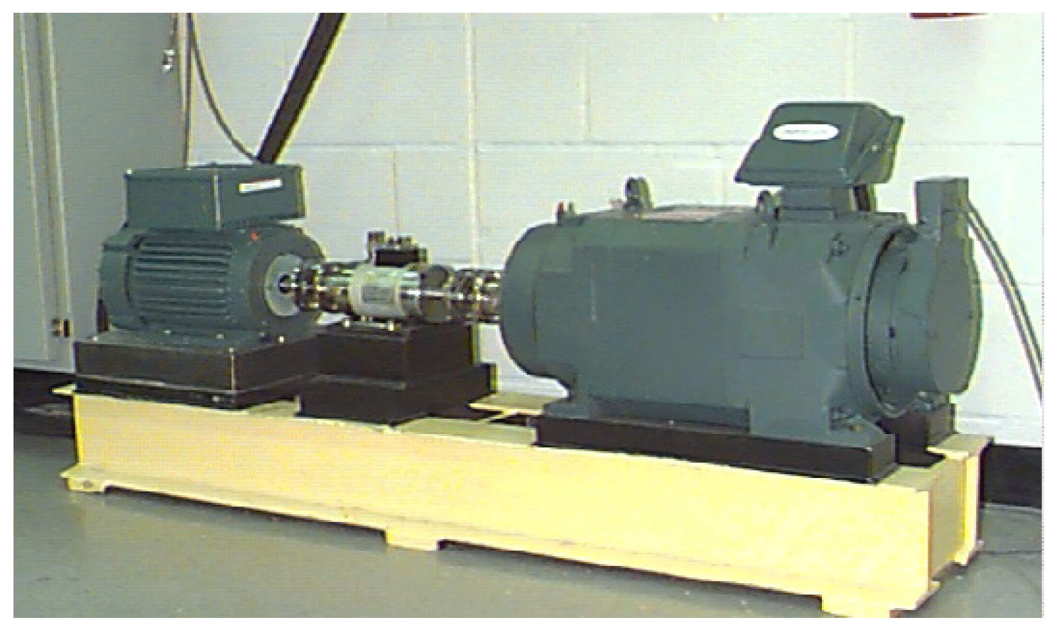
In this case, the proposed method was validated by using the bearing dataset from the Case Western Reserve University (CWRU) [42]. Figure 9 displays the testbed for data collection. The CWRU experiment apparatus mainly consists of an induction motor, rolling bearings, a torque transducer, and a dynamometer. The types of bearing states can be classified as normal (N), inner-race fault (IF), ball fault (BF), and outer-race fault (OF), respectively. The diameters of each fault are 0.1778 mm, 0.3556 mm, and 0.5334 mm. The experimental data were chosen from the drive end and fan end with a sampling frequency of 12 kHz. In total, ten bearing working states under the motor load of 0 hp were analyzed.

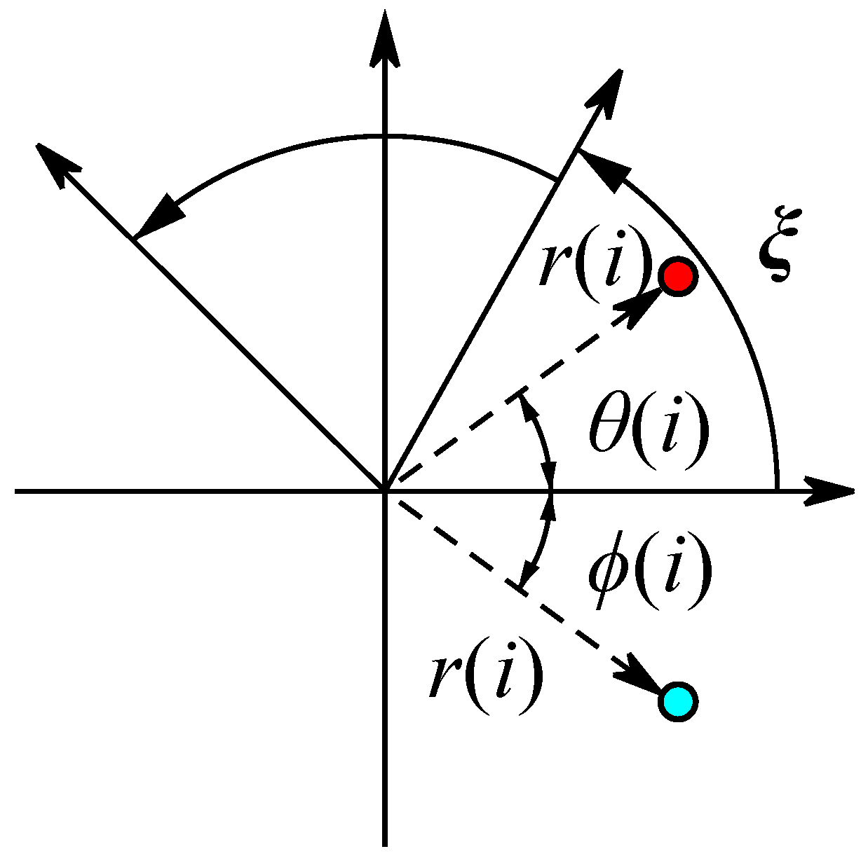
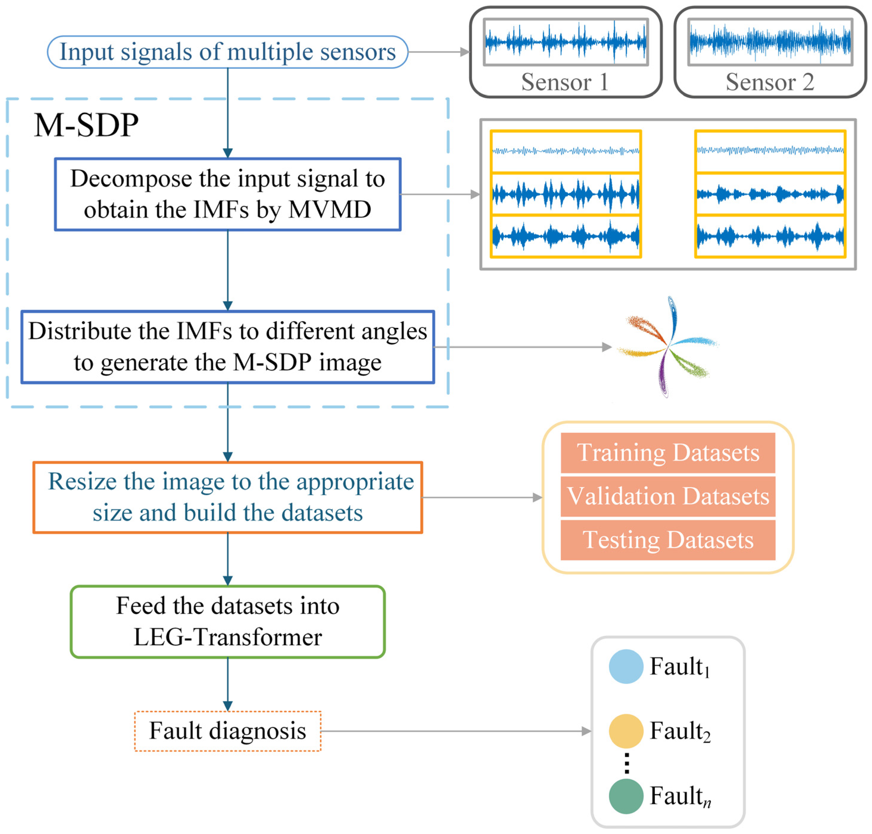
This subsection processes data from two sensors through the proposed M-SDP approach. To ensure the integrity of the individual fault features, the information collected on the drive end with the fan end was fused. Firstly, the raw fused vibration signals were divided into sub-sequence signals of equal length, containing 2048 sampling points. Secondly, a series of feature data were obtained at different scales by co-processing the information from two sensors through the MVMD method. Subsequently, the feature data of different scales were arranged at different angles to gain the M-SDP images, which realized the fusion of multisensor and multiscale information. However, the choice of internal parameters γ, ξ, and L can affect the difference between each M-SDP image. Therefore, the parameters should be selected appropriately. The M-SDP datasets of outer race fault were used to analyze the parameters selection. Since we adopted 2 channel vibration signals and the number of the decomposed number was set to 3 when using MVMD, 6 IMFs needed to be mapped to the polar coordinate system, thus γ was set at 60°. 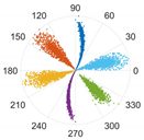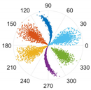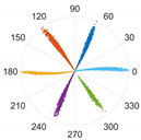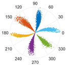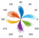Moreover, L was set to 1, 5, and 10, and ξ was set to 10°, 30°, and 50°, respectively. The above parameters were combined to generate nine M-SDP images, as shown in

Table 2. M-SDP images with different internal parameters.

	State: Outer Race Fault
	ξ = 10°	ξ = 30°	ξ = 50°
L = 1
L = 5
L = 10

.

As displayed in Table 2, the differences in shape characteristics, thickness, and curvature of each arm in the M-SDP image can be reflected by changing ξ and L. Specifically, the rotation angle of arms along the initial line gradually increased with the increase in parameter ξ and the thickness of each arm increased slightly with ξ. If the rotational curvature and the thickness of the arms were too small, it reduced the area of recognized features, and the points on the edge of each arm were scattered when they were too large. The above situation can bring obstacles to image classification. Hence, it is particularly important to select appropriate values of ξ and L.

In order to further select the optimal parameters, the normalized cross-correlation coefficient (NCC) method was adopted in this work. For two images M and N, with the same size a × b, the NCC can be expressed by

$$R_{\left(\theta ,g,L\right)}\left(M,N\right)=\frac{{\displaystyle \sum {\displaystyle \sum \left(M_{ab}-\overline{M}\right)\left(N_{ab}-\overline{N}\right)}}}{\sqrt{\left[{\displaystyle \sum {\displaystyle \sum {\left(M_{ab}-\overline{M}\right)}^2}}\right]\left[{\displaystyle \sum {\displaystyle \sum {\left(N_{ab}-\overline{N}\right)}^2}}\right]}}$$

(19)

where $\overline{M}$ and $\overline{N}$ denote the average value of the three channels of image M and N, respectively. The value of R can be used to measure the similarity of two M-SDP images. R ranges from 0 to 1, and the higher the value of R is, the more similar the images of M and N are. The value of L is identified by traversing the interval of [1,10] at step size 1, and the value of ξ is identified by traversing the interval of [20,50] at step size 5. Since there are ten fault types in our datasets, a 10 × 10 matrix can be obtained by calculating the correlation coefficient between every two M-SDP images. Then, the average correlation coefficient of the matrix can be calculated, which is considered the correlation coefficient of ten M-SDP fault images under the current combination of ξ and L. Following this, the non-correlation degree (NR) was further calculated, and the results are displayed in

Table 3. Non-correlation value under different parameters of ξ and L.

	ξ = 20°	ξ = 25°	ξ = 30°	ξ = 35°	ξ = 40°	ξ = 45°	ξ = 50°
L = 1	0.281	0.332	0.452	0.463	0.468	0.474	0.409
L = 2	0.285	0.325	0.364	0.400	0.386	0.389	0.380
L = 3	0.295	0.335	0.373	0.410	0.446	0.421	0.396
L = 4	0.321	0.358	0.423	0.456	0.442	0.438	0.412
L = 5	0.332	0.373	0.421	0.458	0.453	0.467	0.457
L = 6	0.325	0.385	0.447	0.461	0.464	0.445	0.451
L = 7	0.351	0.392	0.452	0.500	0.495	0.490	0.443
L = 8	0.341	0.396	0.449	0.499	0.451	0.448	0.431
L = 9	0.348	0.381	0.459	0.497	0.444	0.428	0.429
L = 10	0.352	0.359	0.438	0.479	0.470	0.446	0.402

. From Table 3, the maximum values of NR correspond to ξ = 35° and L = 7.

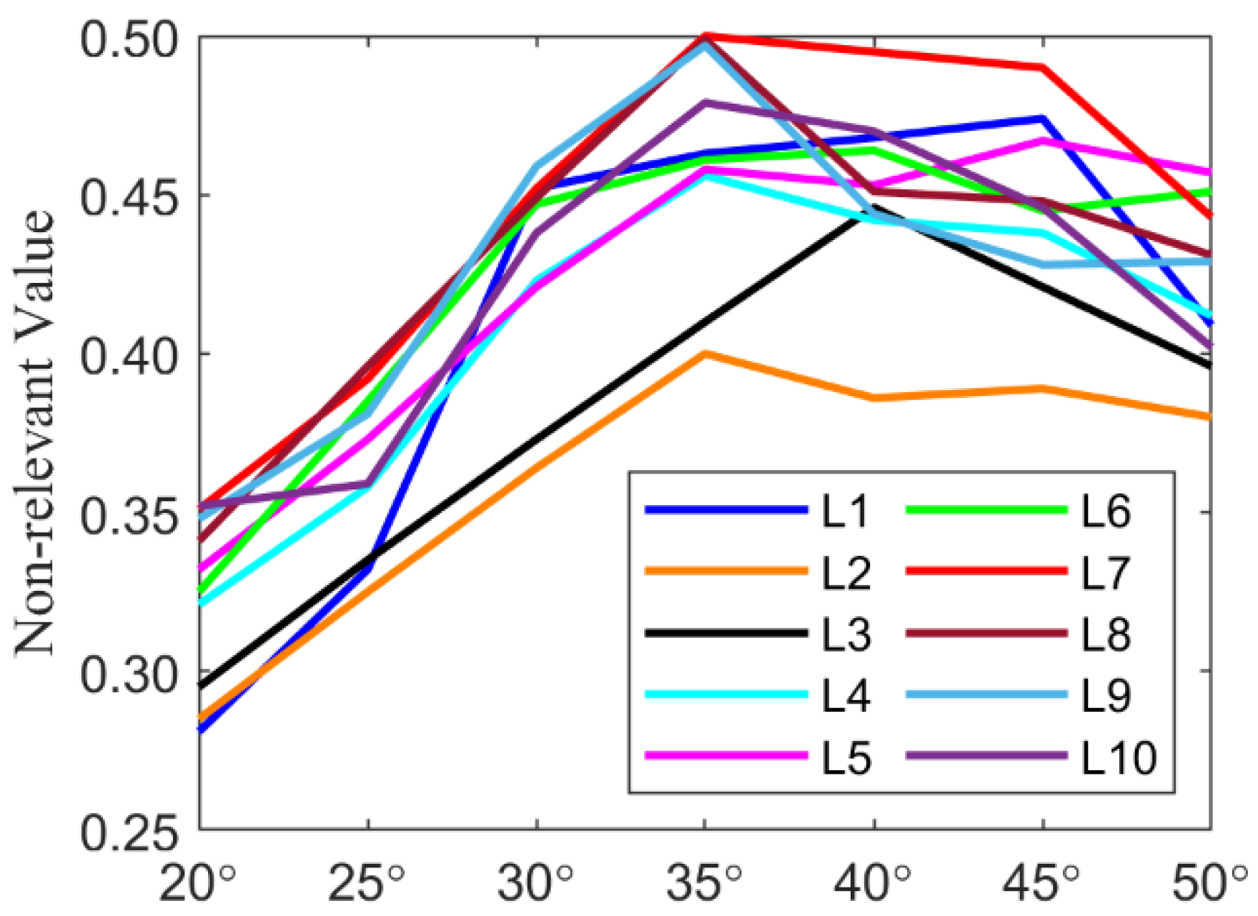
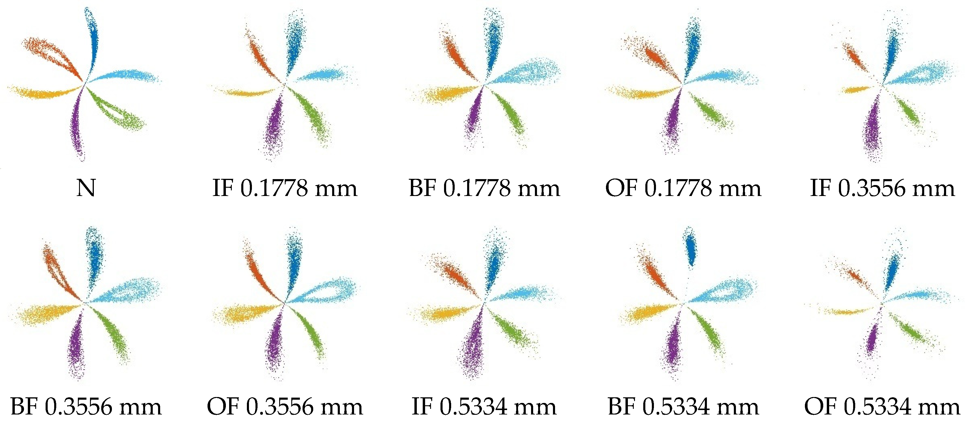
The relationship between NR and the parameters ξ and L can be directly reflected in Figure 10. From Figure 10, when the range of ξ is from 20 to 35, the value of NR increases gradually, but it declines gradually when ξ is between 35 and 50. When ξ is fixed, there is usually a peak of NR at L = 7. Thus, ξ and L are eventually determined by 35 and 7, respectively. 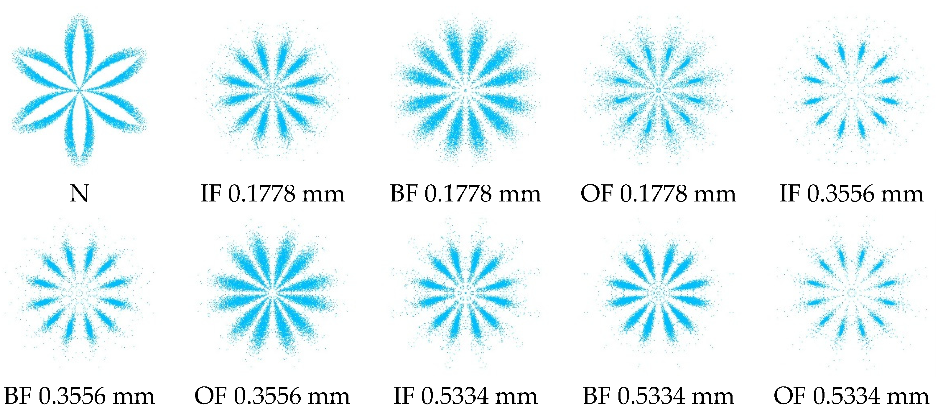According to the selected parameters, the ten types of M-SDP data obtained are shown in Figure 11. Meanwhile, to confirm the effectiveness of the M-SDP method, the single sensor data are processed using the original SDP method as a comparison, and ten types of SDP data are obtained as shown in Figure 12.

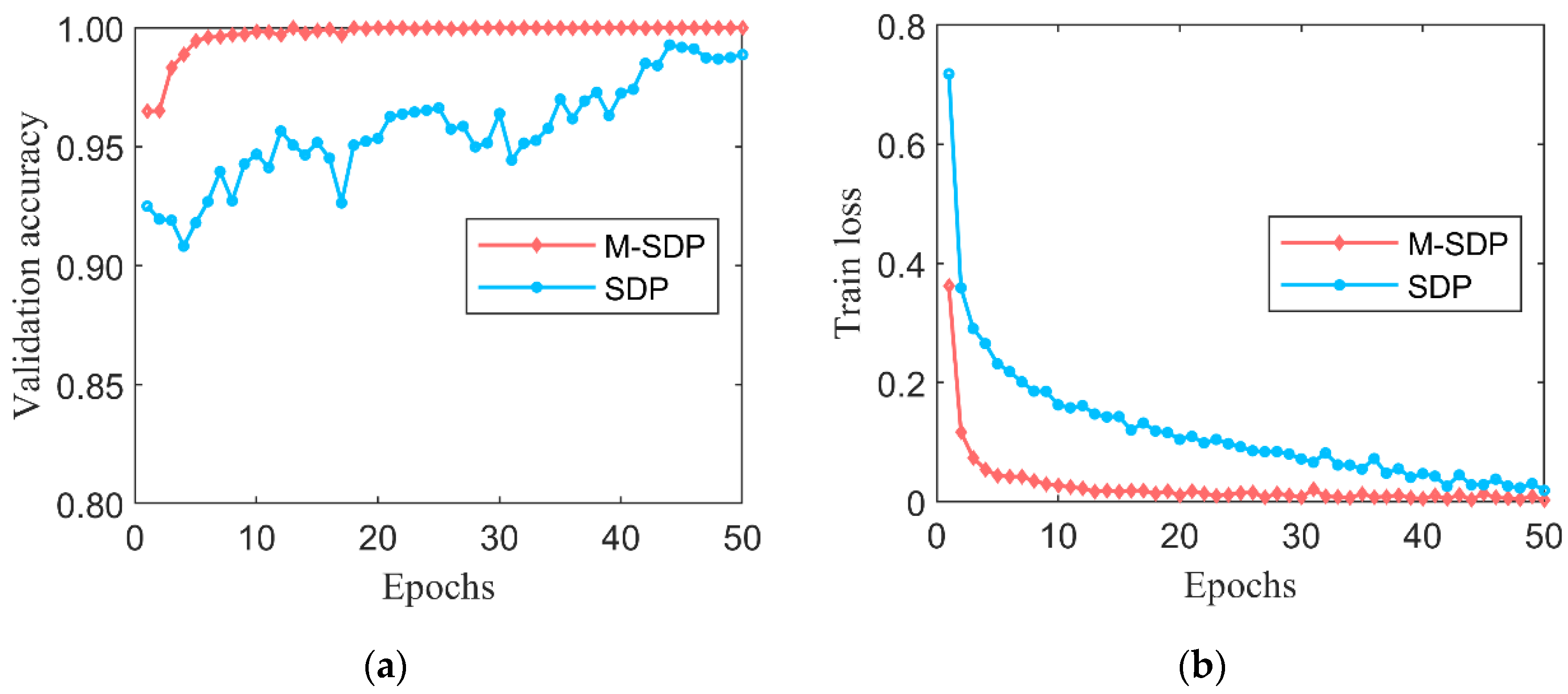
The M-SDP and SDP datasets were randomly divided to validate the diagnostic accuracy of the M-SDP method. Each bearing working condition contains 2000 samples as a training dataset, 400 samples as a validation dataset, and 100 samples as a testing dataset. The LEG Transformer designed in this paper was performed to process the prepared datasets. The initial learning rate of the model is 0.001 and the training epoch is 50. The accuracy of the obtained validation dataset is shown in Figure 13a, and the loss curve is shown in Figure 13b. According to the validation accuracy curves of M-SDP and SDP in Figure 13a, the validation accuracy starts to stabilize and remains around 100% when the training epoch reaches 16. However, the accuracy of the original SDP method is still low and fluctuates wildly before the epoch training reaches 30. From Figure 13b, it can be noticed that the loss of the M-SDP dataset also drops to very low level at epoch 10, while the original SDP has higher loss values than our proposed M-SDP method in all 50 epochs. To further ensure the reliability of the experimental results, the trained model was applied to the pre-prepared testing dataset, and the results include accuracies and standard deviation (SD) as shown in

Table 4. The testing results using M-SDP and SDP (%).

Methods	Max	Min	Mean	SD
M-SDP	100.00	100.00	100.00	0
SDP	99.11	98.76	99.06	0.16

. The M-SDP datasets have no false diagnoses during testing and show superior diagnostic stability with an average accuracy of 100%.

The above results clearly show that the M-SDP method has a compelling improvement over the original SDP, especially in accuracy and stability during training. In the industrial field, real-time fault monitoring is highly required for the efficiency and stability of diagnosis. Accidental misdiagnosis will still have a particularly negative impact on mechanical equipment. The dataset generated by the M-SDP method proposed in this paper has a fast convergence performance during training, and the diagnostic accuracy of the trained model is exceptionally high. The results demonstrate that the M-SDP method can further amplify the differences between categories while making the characteristics of each category more significant.

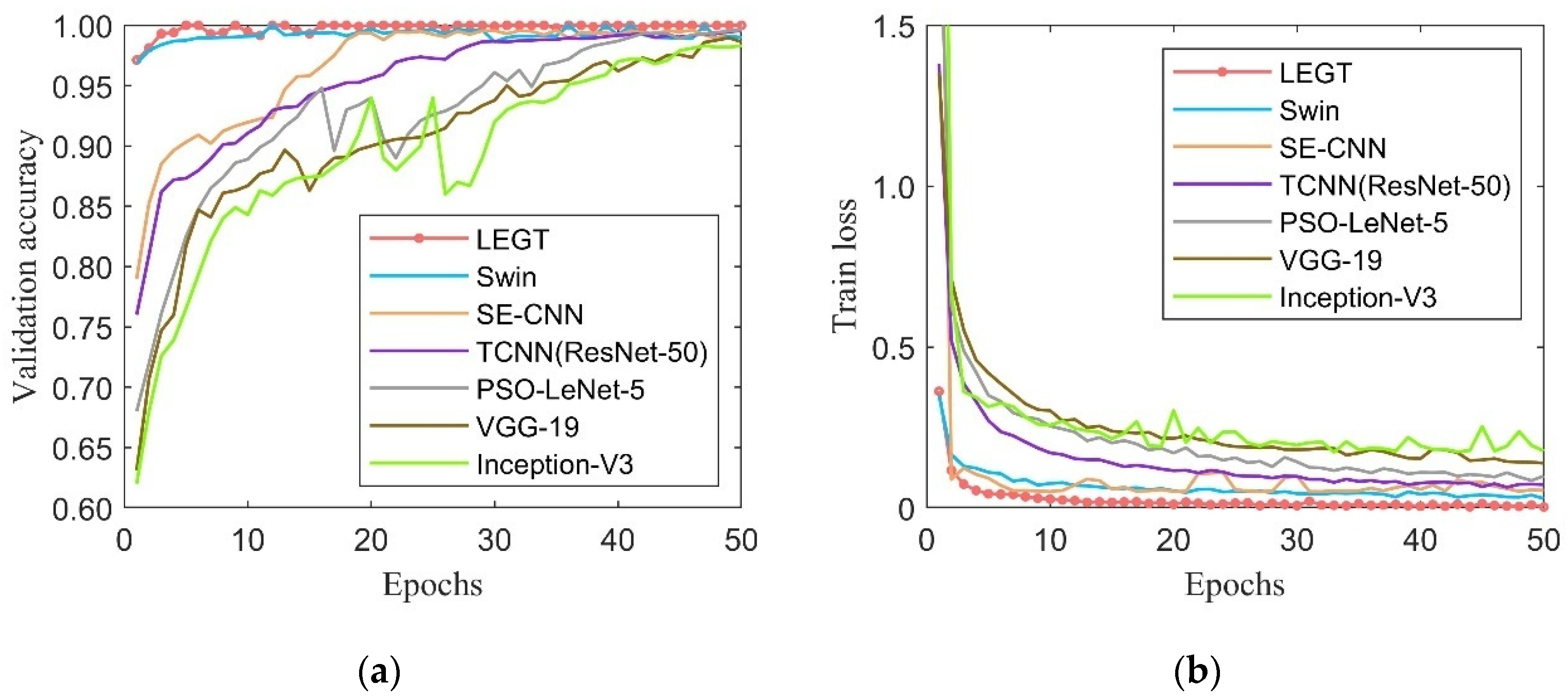
To further validate the performance of the LEG Transformer (LEGT) model exploited in this paper, it was compared with the typical Swin Transformer method for different processes. According to the analysis in the official paper of the Swin Transformer, the model trained with pre-trained weights offered by officials can achieve better recognition accuracy. For this reason, this paper introduced the pre-trained weights in model training. At the same time, more extensive comparisons were made with SE-CNN, TCNN (ResNet-50), PSO-LeNet-5, VGG-19, and Inception-V3 models. The pre-prepared M-SDP datasets were used for fault diagnosis of each deep learning model. Besides, a machine learning method named the particle-swarm-optimization-based support vector machine (PSO-SVM) was implemented to evaluate the necessity of deep learning methods [43]. Figure 14 presents the accuracy and loss of the LEG Transformer and the typical Swin Transformer in the training process.

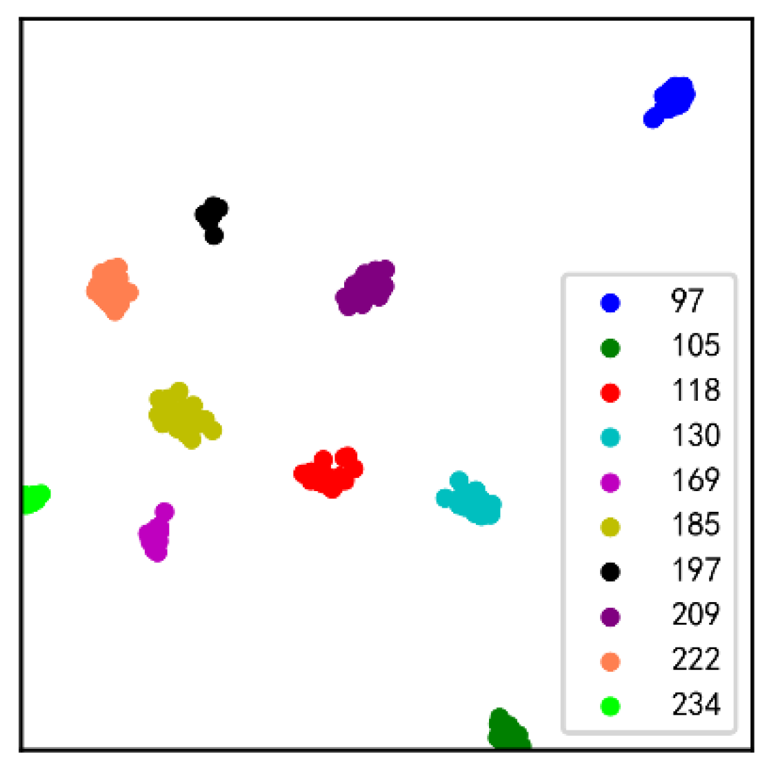
The designed LEG Transformer method achieves the desired effect at about 10 epochs during the training process. In addition, the convergence speed is significantly enhanced compared with before the improvement. The accuracy of the validation dataset and the training loss for deep learning models are shown in Figure 15. From Figure 15, LEG Transformer outperforms other models in recognition accuracy over 50 epochs and has the best stability for fault diagnosis. The LEG Transformer and the Swin Transformer have higher accuracy and convergence speed than other CNN-based models, demonstrating the excellent performance of transformer-based structural models. To show the classification effect of the LEG Transformer more intuitively, the classification results are visualized using the T-distributed stochastic neighbor embedding (t-SNE) method [44], as presented in Figure 16. From the t-SNE figure, it can be observed that the LEG Transformer can effectively separate different features. To further verify the performance of the LEG Transformer model, each model was applied to the testing dataset. 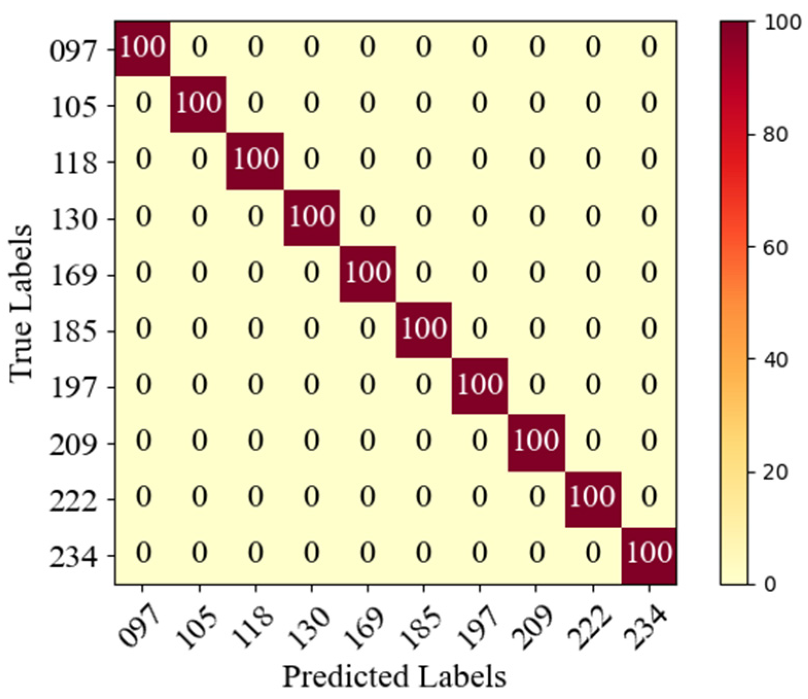Figure 17 shows the confusion matrix of LEG Transformer in processing the testing dataset. The accuracy of each model applied to the testing dataset is shown in

Table 5. The results of the testing dataset in different models (%).

Methods	Max	Min	Mean	SD
LEG Transformer (LEGT)	100.00	100.00	100.00	0
Swin Transformer (Swin)	100.00	99.95	99.97	0.02
SE-CNN	99.99	99.36	99.67	0.19
TCNN (ResNet-50)	99.79	99.21	99.58	0.16
PSO-LeNet-5	99.62	98.99	99.57	0.21
VGG-19	99.96	97.89	98.68	0.72
Inception-V3	99.38	97.23	98.71	0.86
PSO-SVM	99.23	95.59	97.39	0.26

.

From Table 5, the LEG Transformer method proposed in this paper achieves up to 100% average accuracy in classifying the testing dataset. At the same time, the standard deviation of the LEG Transformer is 0. The accuracy values of the Swin Transformer, SE-CNN, TCNN(ResNet-50), PSO-LeNet-5, VGG-19, Inception-V3, and PSO-SVM are 99.97% ± 0.0002, 99.67% ± 0.0019, 99.58% ± 0.0016, 99.57% ± 0.0021, 98.68% ± 0.0072, 98.71% ± 0.0086, and 97.39 ± 0.0026, respectively.

Table 6. Comparative results published in the literature.

Reference	Methods	Accuracy (%)
Present work	LEG Transformer (LEGT)	100.00
Liu et al. [36]	Swin Transformer (Swin)	99.97
Wang et al. [17]	SE-CNN	99.81
Wen et al. [29]	TCNN (ResNet-50)	99.99
Zhu et al. [32]	PSO-LeNet-5	98.71
Simonyan et al. [45]	VGG-19	98.68
Szegedy et al. [46]	Inception-V3	98.71
Yan et al. [43]	PSO-SVM	97.08

shows the comparative result of all models published in the literature. The results reveal that the LEG Transformer outperforms the other models. In conclusion, the proposed LEG Transformer method has superior diagnostic accuracy and stable performance.

5.2. Case 2

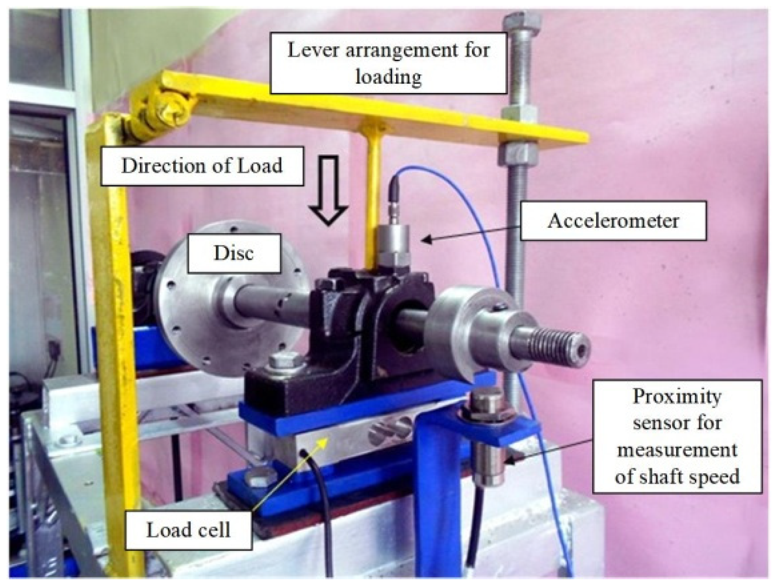
To further analyze the generalization capability and robustness of the proposed LEG Transformer model, this case employed it with a new dataset for testing and comparison. Figure 18 displays the testbed for data acquisition and the roller bearing NU205E was chosen as the experimental bearing [47]. The vibration signals were collected at a shaft speed of 2050 rpm and a load of 200 N. In this case, the vertical channel and the horizontal channel of the data acquisition device were adopted. The dataset composition that contains twelve fault types is specifically demonstrated in

Table 7. The composition of the dataset.

Bearing State	Label	Fault Size (mm)
Inner-race fault	A1	0.43
	A2	1.01
	A3	1.56
	A4	2.03
Outer-race fault	B1	0.42
	B2	0.86
	B3	1.55
	B4	1.97
Ball fault	C1	0.49
	C2	1.16
	C3	1.73
	C4	2.12
Normal	N	-

.

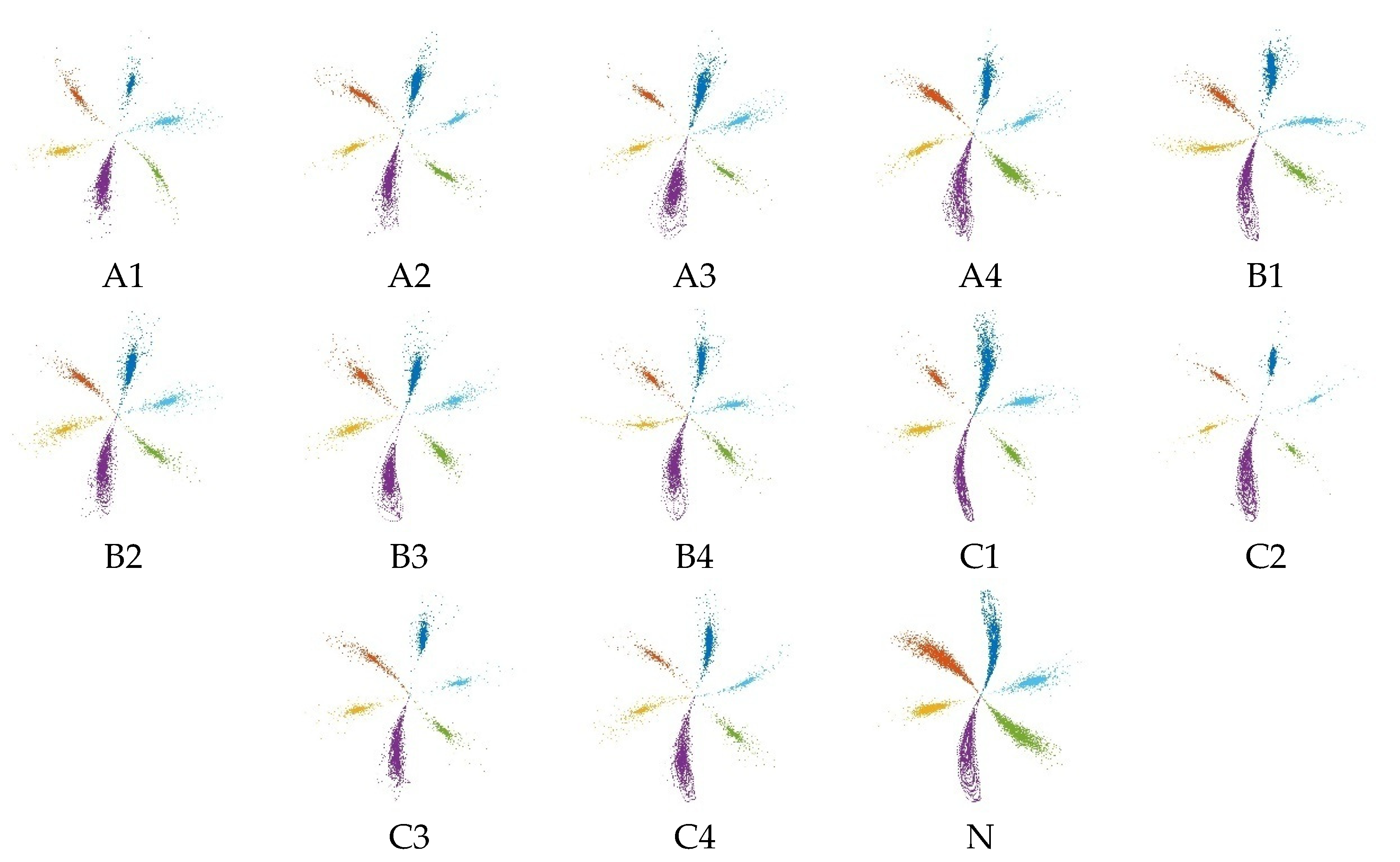
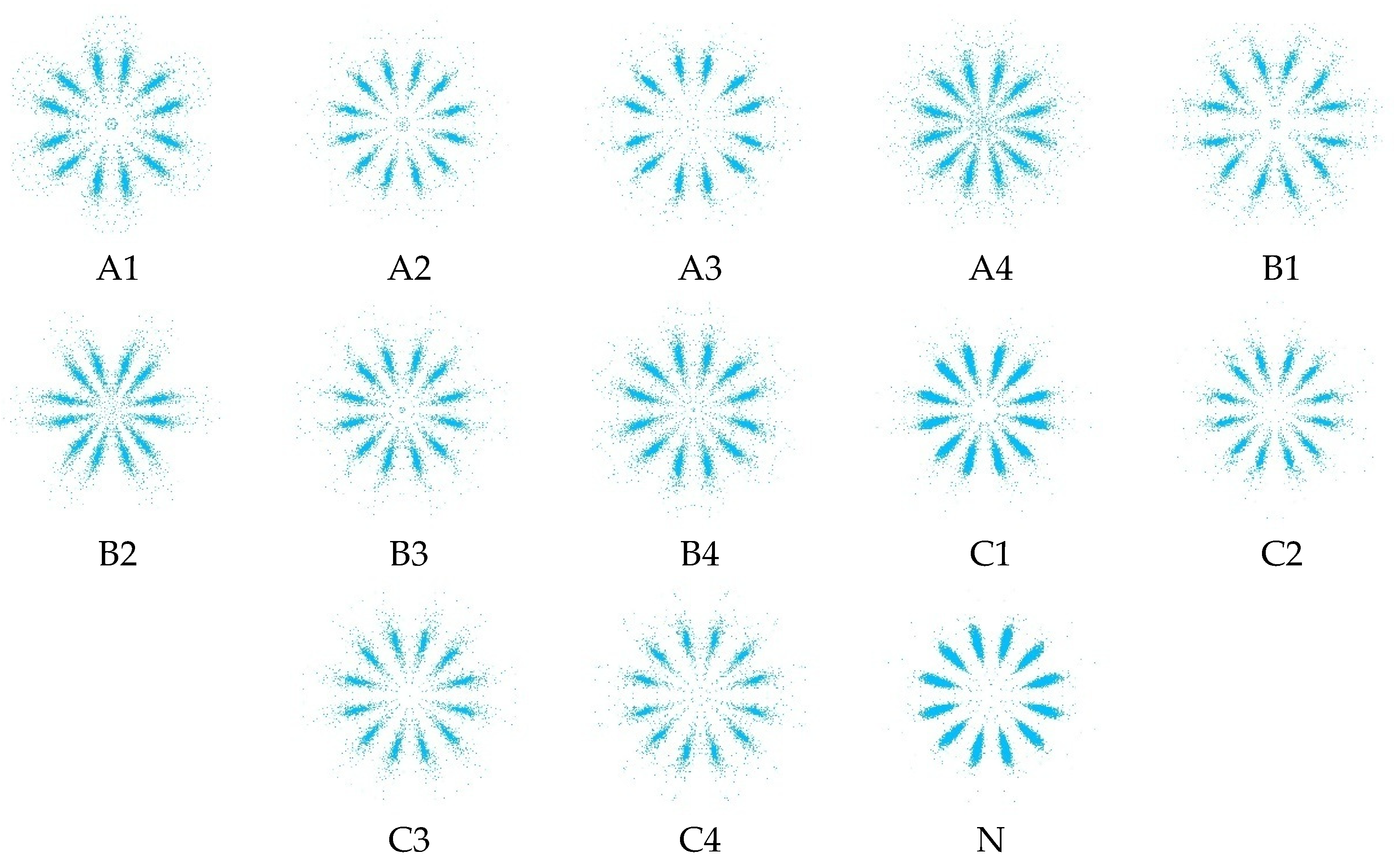
In this case, the procedure to select internal parameters and form the M-SDP datasets is similar to Case 1. The M-SDP images for the thirteen types of bearing states are displayed in Figure 19. The original SDP images as a comparison are presented in Figure 20.

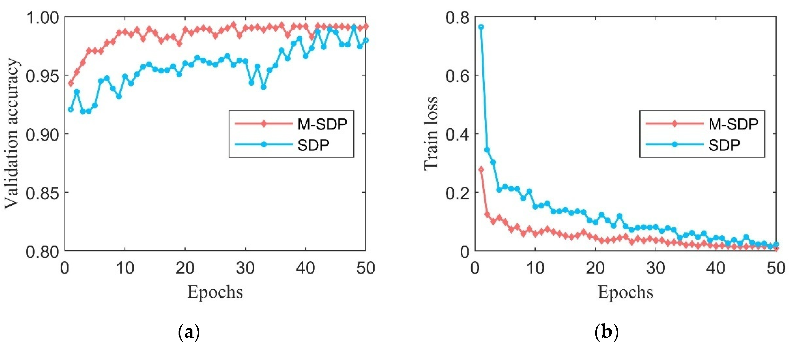
The M-SDP and SDP datasets are randomly split, with 2000 samples of each category as a training dataset, 400 samples as a validation dataset, and 100 samples as a testing dataset. The proposed LEG Transformer was implemented on the prepared datasets. The accuracy of the validation dataset of M-SDP and original SDP during training is displayed in Figure 21a, and the loss curve is shown in Figure 21b.

In the M-SDP datasets of this case, Figure 21a,b demonstrate a significant advantage in the accuracy of the validation dataset compared with the original SDP. For different kinds of bearing states, the datasets obtained by the M-SDP method have a fast convergence speed and excellent stability of correct classification.

Table 8. The testing results using M-SDP and SDP (%).

Methods	Max	Min	Mean	SD
M-SDP	99.63	97.34	99.07	0.26
SDP	99.35	96.57	98.01	0.46

demonstrates the experimental results for the testing dataset. From Table 8, the diagnostic effect of the M-SDP datasets is better than the original SDP method in this process.

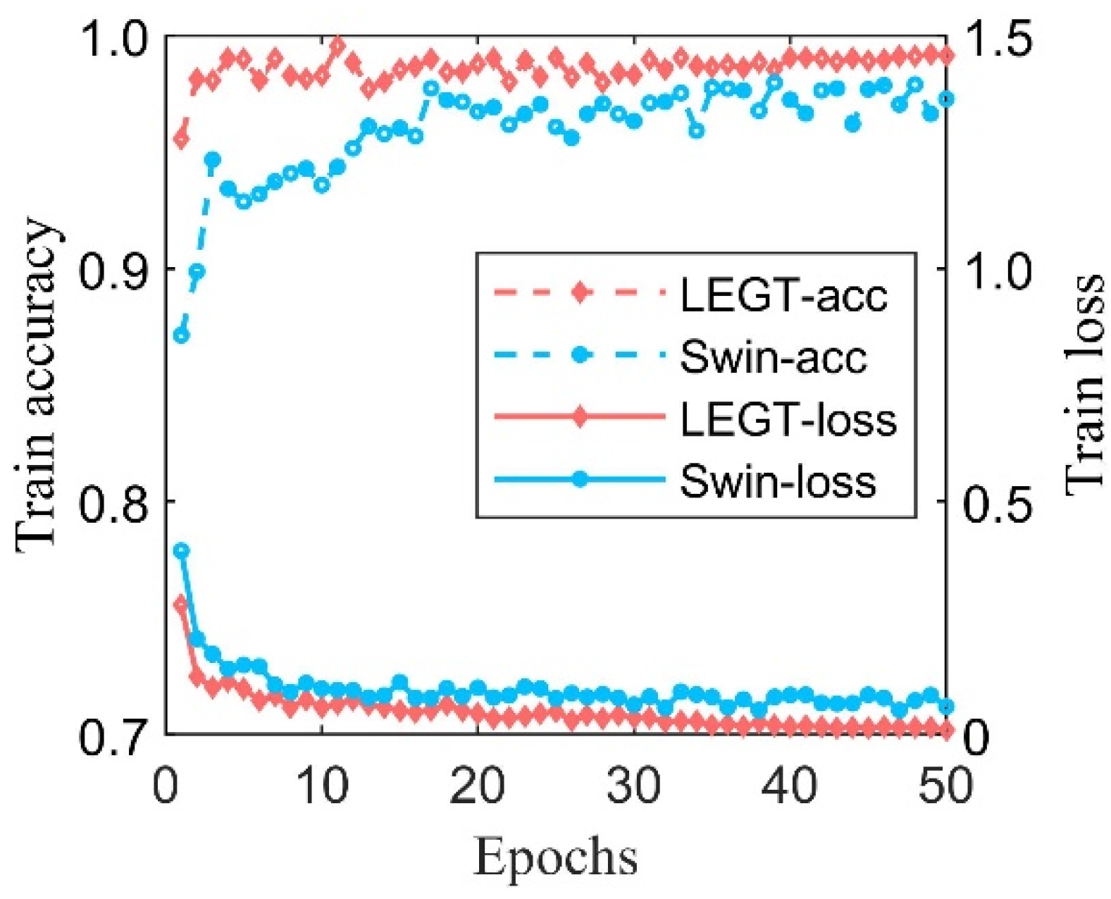
In this case, the proposed LEG Transformer (LEGT) was compared with the Swin Transformer, SE-CNN, TCNN (ResNet-50), PSO-LeNet-5, VGG-19, Inception-V3, and PSO-SVM models. The accuracy and loss curves of the LEG Transformer and the original Swin Transformer in the training process are shown in Figure 22.

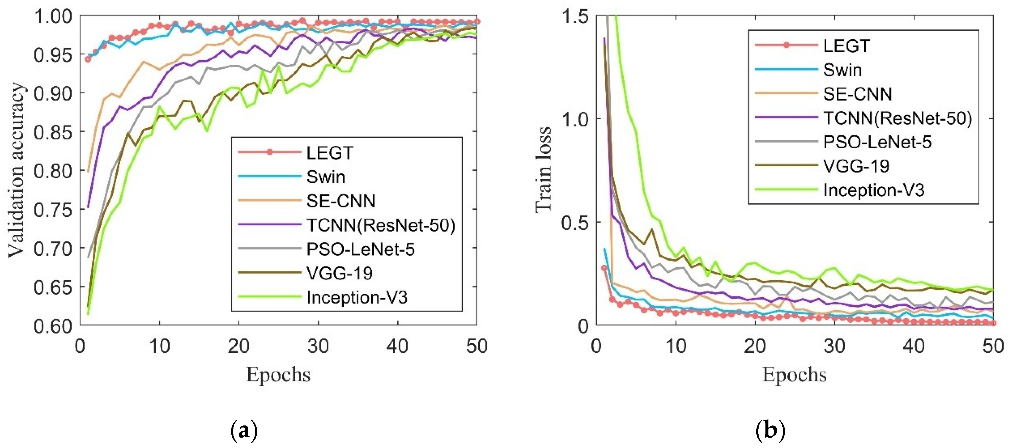
Similarly, the LEG Transformer showed significantly improved diagnostic performance over the original Swin Transformer. The accuracy of the validation datasets for deep learning models and train loss are shown in Figure 23.

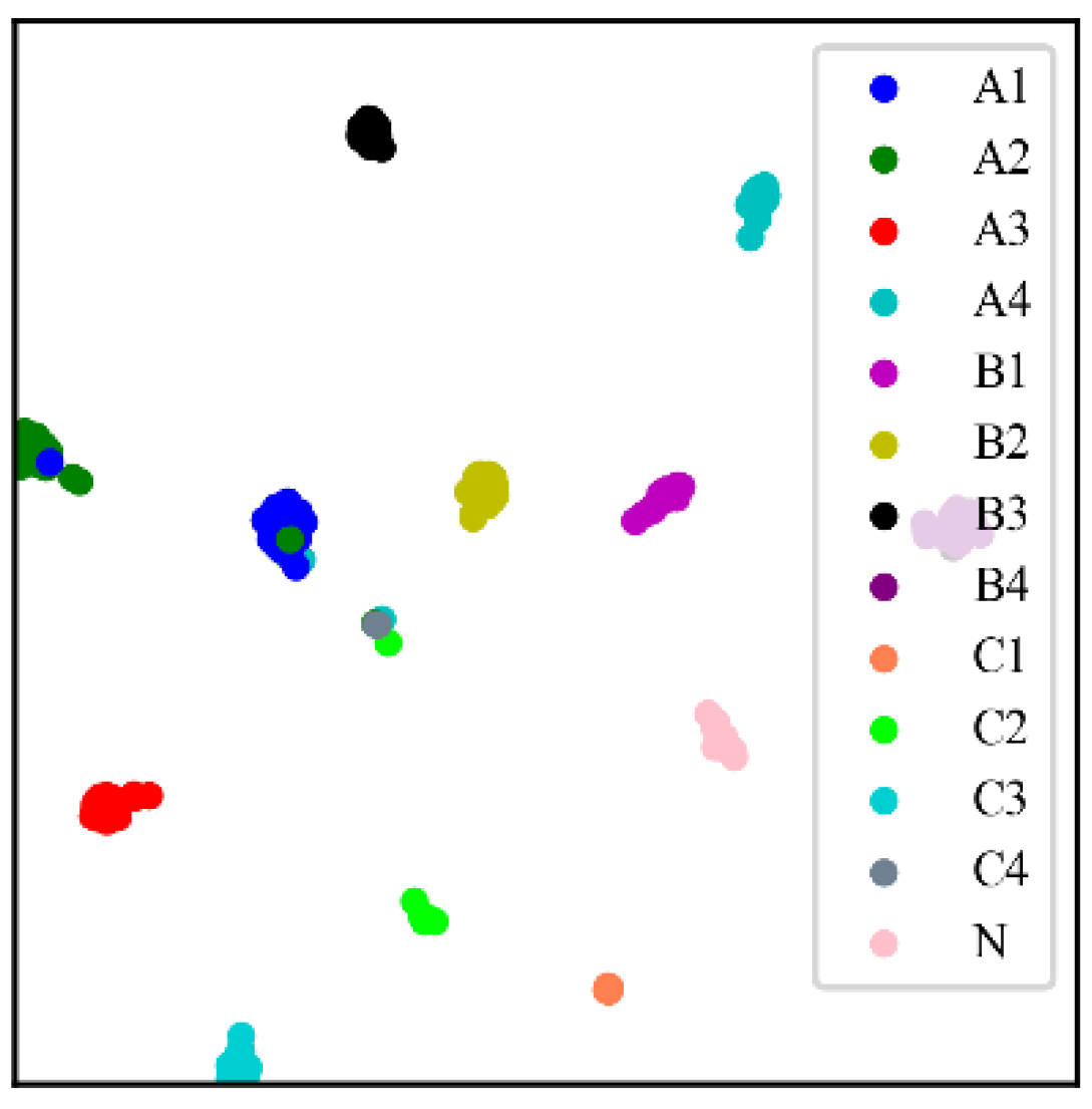
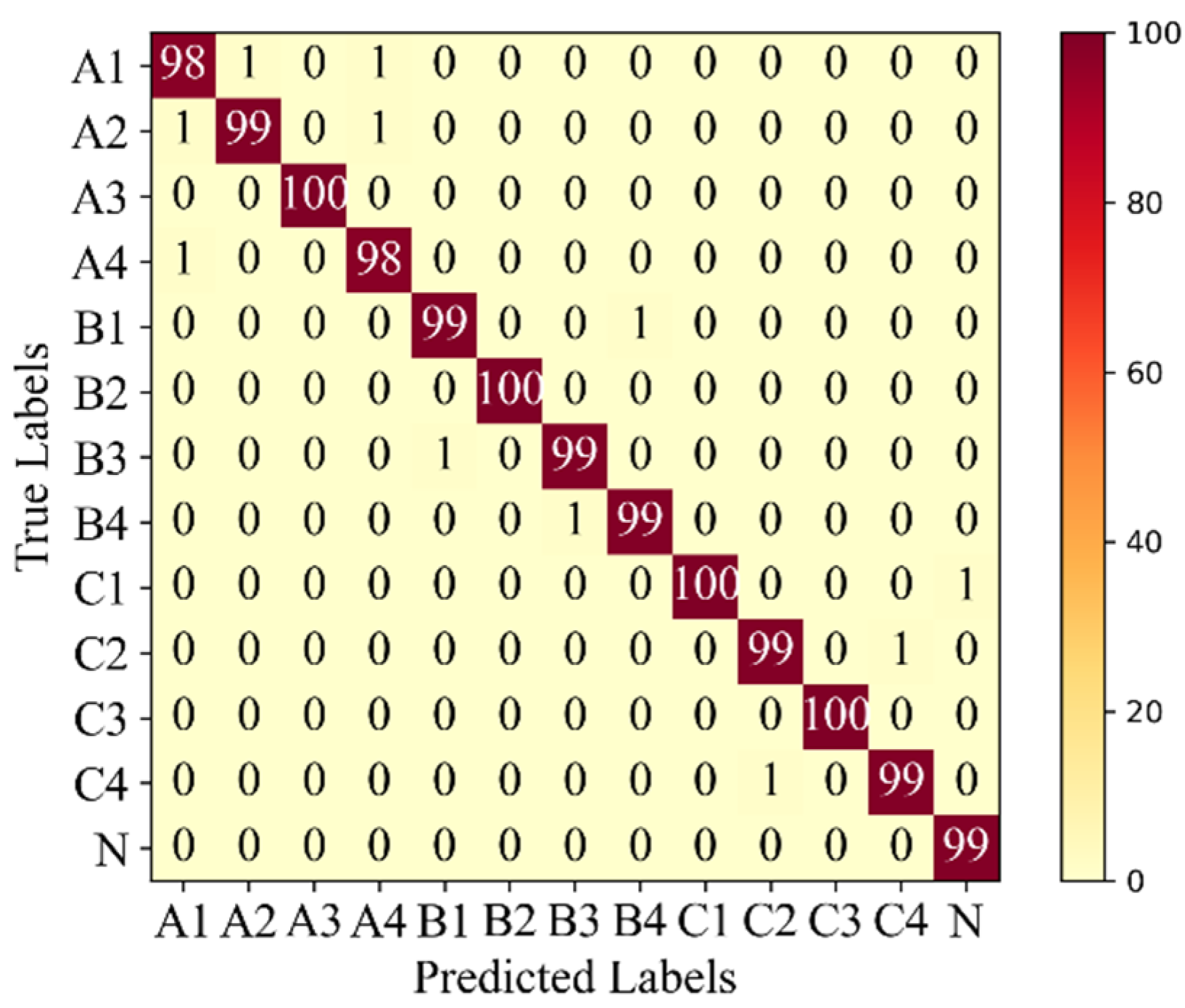
Similar to the dataset in Case 1, the LEG Transformer is still the best among all models in classification accuracy and fault diagnosis stability. The LEG Transformer visualization of the classification results for this section of the dataset is illustrated in Figure 24. The confusion matrix of LEG Transformer is shown in Figure 25. The classification results of the testing dataset for each model are shown in

Table 9. The results of the testing dataset in different models (%).

Methods	Max	Min	Mean	SD
LEG Transformer (LEGT)	99.67	98.78	99.15	0.14
Swin Transformer (Swin)	99.03	97.84	98.95	0.21
SE-CNN	98.88	98.28	98.67	0.20
TCNN (ResNet-50)	98.57	97.68	98.10	0.35
PSO-LeNet-5	98.44	96.62	97.86	0.38
VGG-19	98.40	96.69	98.01	0.76
Inception-V3	97.71	95.89	97.23	0.84
PSO-SVM	98.26	94.63	96.98	0.67

.

The LEG Transformer has superior performance when dealing with different datasets, and these results indicate that the model has strong generalization ability and robustness.

6. Conclusions

This study presents a bearing fault diagnosis method based on M-SDP and the LEG Transformer. The proposed M-SDP method ensures the integrity and richness of bearing condition information by taking advantage of MVMD and SDP. SDP was applied to visualize the multisensor and multiscale information. Compared with SDP, the M-SDP method was proven to be better in expressing the difference between various features in processing vibration signals and significantly improves the diagnostic accuracy and stability during testing in two datasets. In addition, this paper effectively combines the local-to-global attention block and the locally enhanced positional encoding mechanism and applies them appropriately to the Swin Transformer framework to satisfy the requirements of bearing fault diagnosis, thus proposing the LEG Transformer. The experimental results demonstrate that the diagnostic accuracy is over 99% of the proposed method in processing testing datasets, indicating that the LEG Transformer has more powerful image processing and feature extraction ability than the typical Swin Transformer. Compared with different CNN-based models, it was found that the LEG Transformer has a higher classification recognition rate, better convergence, and the best stability. All the above results confirm the validity and reliability of the proposed LEG Transformer method.

In future research, the fusion of more signal channels will be considered, and the effectiveness of the proposed bearing fault diagnosis method will be validated.