Research on Milling Characteristics of Titanium Alloy TC4 with Variable Helical End Milling Cutter

Abstract

The application of variable helical end mills to the milling of titanium alloys can suppress the regeneration effect during the machining process and ensure the stability of milling. However, due to their special geometry, their milling characteristics are also different. In this paper, the process of milling titanium alloy with a variable helix end mill is taken as the research object, and the milling force, milling stability and machining effect during the machining process are deeply studied. Firstly, the feed per tooth and cutting thickness model of the variable helical end mill were established, the milling force prediction model of the variable helical end mill was deduced, and the instantaneous milling force and its variation law were obtained by solution. Secondly, the finite element analysis model of the variable helix end mill for machining titanium alloy was established, and the influence of the variable helix angle structure on the milling force was obtained. Then, the dynamic equation of milling with a variable helix end mill was established, the stability lobe diagram of variable helix milling is was and drawn, and the influence of variable helix angle on milling stability was analyzed. Lastly, a variable helix end mill milling experiment was designed to verify the accuracy of the theoretical model and finite element simulation; the influence of the variable helix angle structure on the surface roughness was analyzed, and the influence of machining parameters on the milling force when using a variable helix end mill was investigated.

1. Introduction

Titanium alloys are widely used in aerospace, ships, automobiles, and molds due to their high strength, good toughness, and corrosion resistance [1]. However, the titanium alloy itself has a small thermal conductivity and poor thermal conductivity, which makes it easily bond with the tool, thus affecting the machining accuracy, and it has low elastic modulus and large elastic deformation. It bends and deforms easily under the action of radial force during processing, and vibration occurs [2]. Because of their nonconstant or alternating helix angle structure, variable helix end mills can effectively suppress the regeneration effect, maintain the stability of milling, and improve the material removal rate [3]. Therefore, the research on the milling characteristics of titanium alloys with variable helical milling cutters has important theoretical significance and practical value for its application in the field of milling of complex structures and difficult-to-machine parts.

In recent years, scholars have carried out some research on the machining mechanism of variable helix end mills, including the establishment and solution of a milling force model, the establishment and stability analysis of a dynamic model, simulation analysis and experimental research, and tool structure optimization.

For the research of milling force, Wang [4] integrated the two structures of variable pitch angle and variable helix angle, and established a prediction model for the milling force of a vibration-reduced milling cutter based on the dual mechanism of shearing and ploughing effects. Huang [5] established a milling force model of a variable pitch end mill in view of the easy vibration and severe tool eccentricity in titanium alloy processing, and optimized the pitch angle according to the principle of spectral energy distribution. Xu [6] designed an experiment to compare the milling force of the variable helical milling cutter and the ordinary milling cutter. The experiment showed that the milling force of the variable helical milling cutter was greater than that of the ordinary milling cutter due to the difference in the helix angle of the side edge. Cui [7] established the milling force model of the variable pitch variable helical milling cutter considering the inter-tooth angle and the helix angle, and analyzed the stability of the nonstandard milling cutter on the basis of the machining dynamic characteristics. Wang [8] established a milling force model of a variable helical milling cutter based on bevel cutting, analyzed the influencing factors of the milling force, and optimized the structure of the variable helical end mill with the uniform distribution of the milling force in the frequency domain as the optimization objective. Compean et al. [9] established a multivariable vibration-damping milling force model based on variable pitch angle and variable helix angle by introducing variable rake angle, and predicted the stability limit by using the enhanced homotopy perturbation method.

For the research on the stability of variable-helix and variable-pitch milling cutters, Liu et al. [10] comprehensively considered the influence of tool wear and cutting speed, and analyzed the influence of the two on the milling stability of variable helix end mills individually and jointly. Shao [11] established a dynamic model of the milling system of a variable pitch end mill, and analyzed the influence of the variable pitch angle and the number of teeth on the milling stability region under different helix angles. Jin [12] transformed the variable time-delay term of the variable pitch characteristic into a multi-delay problem, proposed a semi-discrete method based on the change of the number of time delays with the state, and analyzed the change of the system stability affected by the variable helix angle. Zhang et al. [13] considered the variation of tooth pitch between different blade elements in the variable helix angle structure, proposed a milling stability prediction model, and analyzed the impact of the milling cutter on the milling stability through milling experiments. Niu et al. [14] proposed a generalized Runge–Kutta method to analyze the stability of variable helix and variable pitch end mills for the multiple regeneration effects caused by tool runout, and discussed the joint effects of tool runout and variable pitch angle structure on milling force and chatter stability. Wang et al. [15] proposed an improved semi-discrete method. By analyzing the milling stability of variable helical milling cutters and variable pitch milling cutters, it was found that the variable helical milling cutter and the variable pitch milling cutter had better suppression effects on chatter. Sellmeier et al. [16] established the multi-constant time-delay differential equation of the variable pitch end mill, and proposed two approximate solutions based on the Ackermann method to determine the stability limit of the variable pitch end mill milling system. Turner et al. [17] predicted the chatter stability of the variable helical milling cutter, compared the stability of the variable helical milling cutter and the variable pitch milling cutter, and found that the variable helical milling cutter had better stability. Hayasaka et al. [18] proposed an improved multifrequency method to predict the stability boundary for variable helix end mills. Compared with the semi-discrete method, the convergence speed was greatly improved, and the prediction accuracy of the stability limit in the low-speed region was improved. Ozkirimli et al. [19] introduced the time-averaged delay term to deal with the multi-delay caused by the variable helix angle structure, and derived a generalized vibration-reduced milling cutter dynamics and stability model based on multi-axis milling.

For the study of tool structure optimization, Sun et al. [20] established the three-dimensional stability lobe diagram of the variable helix end mill based on the variable helix angle structure, and used a time-domain simulation method to optimize the variable helix angle parameters. Wang [21] deduced the dynamic models of three types of vibration-damping milling cutters, and carried out the optimal design of three vibration-damping structures using a numerical analysis method. Comak et al. [22] proposed a practical and accurate tool design method for selecting the optimal combination of pitch and helix angle, which could significantly increase the stable cutting limit depth. On the basis of a five-axis variable pitch ball nose milling system, Zhan et al. [23] established a multi-delay comprehensive dynamic model, used the extended SDM method to solve the stability limit, and optimized the pitch angle. Stepan et al. [24] proposed a numerical optimization method for variable pitch angle, which could obtain the geometric parameters of the tool with better vibration-damping performance within the given process parameter range. Ahmad et al. [25] adopted the semi-discretization method to optimize the design of the variable-helix end mill by adjusting the helix and the geometry of the variable-pitch tool, and analyzed the influence of the optimized structure on the milling stability through experiments. Urena et al. [26] introduced the robust and chatter-free design index of variable helix end mills, obtained the index threshold theoretically, and proposed a general design method of variable helix end mills. Takuya et al. [27] proposed a variable helix end mill design method that can achieve robust regeneration suppression, established a unique relationship between the quantitative influence index of the regeneration effect quantization factor and variable helix angle structure, and optimized the geometry of the variable helix end mill.

In summary, scholars have carried out a series of studies on the structural characteristics of variable helix end mills, and have achieved some results in milling stability research and tool structure optimization. However, there are few studies on the milling force characteristics of variable helix end mills, and there is no systematic research on the milling force and machining effect of variable helix end mills. Therefore, it is necessary to conduct in-depth research on the milling force model and its influencing factors. In this paper, a variable helix end mill with different helix angles of each cutting edge and a constant helix angle on the same cutting edge was taken as the research object, the prediction model of milling force of variable helix end mill was established, the model was solved, and the variation law of milling force was analyzed. According to the material failure criterion, a finite element simulation model of variable helical cutter milling titanium alloy was established, and the influence of variable helical angle structure on the milling force was further analyzed. Combined with the process damping effect, the milling stability of the variable helix end mill was analyzed. Lastly, a milling experiment was designed to verify the accuracy of the theoretical model and the finite element simulation model.

2. Establishment and Solution of Milling Force Model

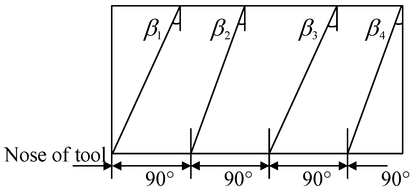
This paper took the four-blade variable helix end mill as the research object. The helix angle of each cutting edge of the research tool was different, and the helix angle of the same cutting edge was unchanged. First, it was assumed that the helix angle of the blade at the symmetrical position of the variable helix end mill was equal (β₁ = β₃, β₂ = β₄), and the pitch angle at the tip was 90°, as shown in Figure 1.

The feed per tooth of the variable helical end mill is related to the tooth pitch between adjacent cutting edges. By discretizing the variable helix end mill along the axial direction, each micro element can be regarded as a variable pitch end mill, and the helix angle of all micro elements is equal. According to the feed per tooth model of the standard milling cutter, the feed per tooth f(i,z) of the i-th cutting edge at height z can be written as:

$$f\left(i,z\right)=\frac{v_f\times \psi \left(i,z\right)}{n\times 2\pi },$$

(1)

where ψ(i,z) is the pitch angle at height z of the milling cutter during the rotation of the i-th cutting edge to the (i + 1)-th cutting edge.

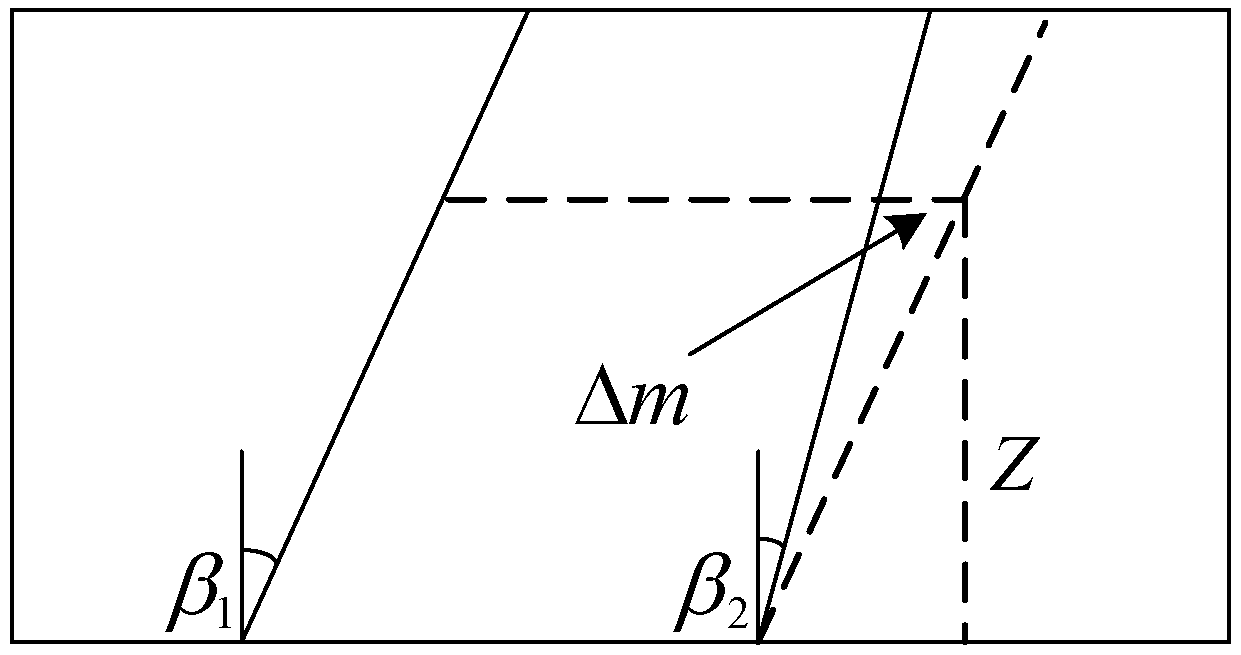
In order to solve the pitch angle function, firstly, the two adjacent cutting edges of the milling cutter were expanded along the circumference, as shown in Figure 2.

Because the helix angles of the two adjacent cutting edges were different, the arc length difference Δm at the height z of the two cutting edges could be written as:

$$\Delta m=z(\tan ({\beta }_1)-\tan ({\beta }_2)).$$

(2)

Substituting the arc length formula Δψ = Δm/R into Equation (2), the pitch angle function can be written as:

$$\psi \left(z\right)={\psi }_0-\frac{z(\tan ({\beta }_1)-\tan ({\beta }_2))}{R},$$

(3)

where ψ₀ is the pitch angle at the end tooth, according to the assumption that ψ₀ = π/2.

Assuming that the helix angle of the i-th cutting edge is β_i, according to the assumption of the variable helix angle structure, the pitch angle function can be written as:

$$f\left(i,z\right)=\frac{v_f}{n\times 2\pi }\{\begin{array}{l}\frac{\pi }{2}-\frac{z\left(\tan {\beta }_1-\tan {\beta }_2\right)}{R}\hspace{1em}i=1,3\hfill \\ \frac{\pi }{2}+\frac{z\left(\tan {\beta }_1-\tan {\beta }_2\right)}{R}\hspace{1em}i=2,4\hfill \end{array}.$$

(4)

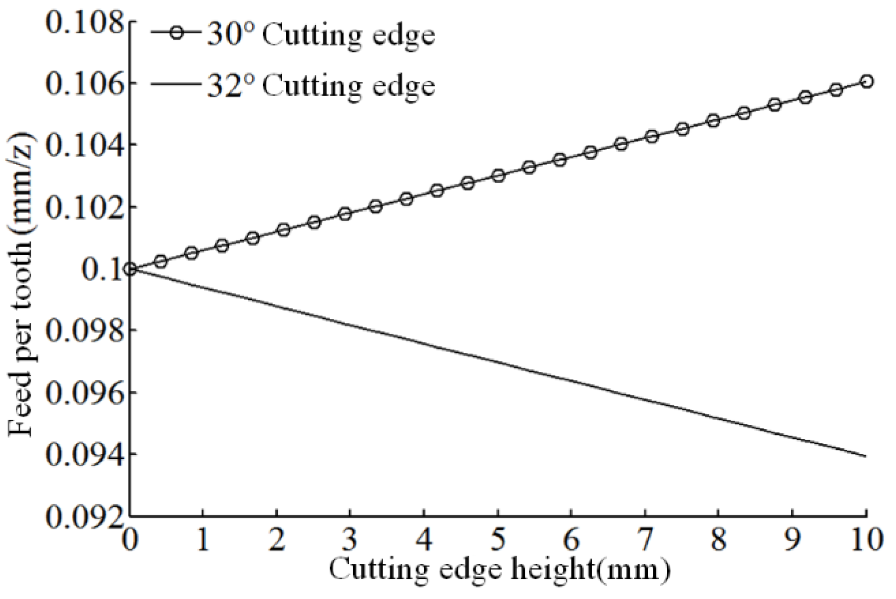
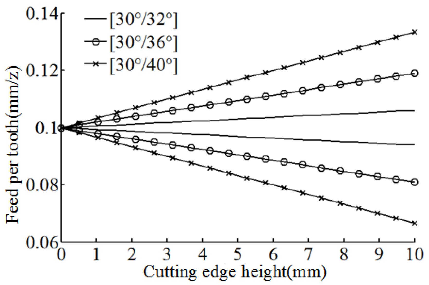
Figure 3 shows the function image of the feed per tooth of the [30°/32°] variable helical end mill. Since the helix angle of the symmetrical cutting edge of the tool was equal, the first two cutting edges were mainly analyzed.

It can be found from Figure 3 that, when the cutting edge with a large helix angle rotates to the cutting edge with a small helix angle, the feed per tooth decreases continuously with the increase in the height of the milling cutter. When the cutting edge with a small helix angle rotates to the cutting edge with a large helix angle, the feed per tooth increases continuously with the increase in the height of the milling cutter. Moreover, the change rate of the feed per tooth of the two cutting edges is equal.

Figure 4 shows the function diagram of the feed per tooth for different variable helix angle structures. It can be found from Figure 4 that, after changing the second helix angle, the change trend of the feed per tooth does not change, and, as the second helix angle increases, the feed per tooth changes more quickly with the height of the milling cutter.

The cutting thickness is related to the feed per tooth and the radial position angle. First, the azimuth angle function was established. Let the turning angle of the cutting edge be θ and the initial azimuth of the first cutting edge be ϕ(i,z). Due to the hysteresis effect of the helix angle, the hysteresis angles at different heights were obtained according to the geometric relationship, and then the direction angle ϕ(i,z) of the edge element at the z height of the i-th tooth on the milling cutter could be written as:

$$\phi \left(i,z\right)=\theta +\phi \left(1,0\right)-(i-1){\psi }_0-\frac{z}{R}\tan \left({\beta }_i\right).$$

(5)

Then, on the i-th tooth, the instantaneous cutting thickness h(i,z) of the micro-element cutting edge at the height z can be written as:

$$h(i,z)=f\left(i,z\right)\sin \phi \left(i,z\right).$$

(6)

Substituting Equations (4) and (5) into Equation (6), the cutting thickness of the cutting edge can be written as:

$$\{\begin{array}{ll}h(i,z)=& \frac{v_f\left[\frac{\pi }{2}-\frac{z\left(\tan {\beta }_1-\tan {\beta }_2\right)}{R}\right]}{n\times 2\pi }\sin \phi \left(i,z\right)\\ & i=1,3\\ h(i,z)=& \frac{v_f\left[\frac{\pi }{2}+\frac{z\left(\tan {\beta }_1-\tan {\beta }_2\right)}{R}\right]}{n\times 2\pi }\sin \phi \left(i,z\right)\\ & i=2,4\end{array}.$$

(7)

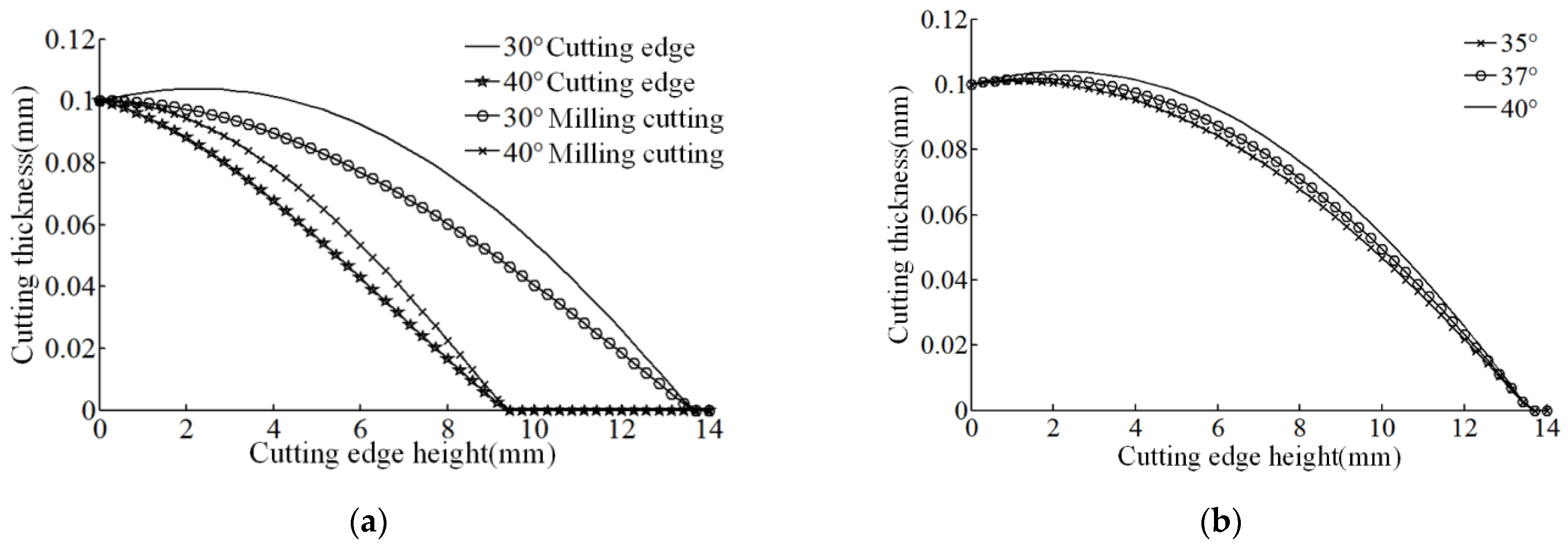
As shown in Figure 5a, the cutting state was selected when the tool nose was rotated 90°, and the plots of different heights of cutting thickness were drawn corresponding to [30°/40°] variable helix end mills and standard end mills with helix angles of 30° and 40°.

It can be found from Figure 5a that, for the variable helix end mill, as the height of the milling cutter increases, the cutting thickness of the cutting edge with the small helix angle (30°) increases first and then decreases, and the cutting thickness of the cutting edge with the large helix angle (40°) decreases monotonically. In the decreasing range of the two curves, the descending speed of the two cutting edges is similar, and, at the same cutting edge height, the cutting thickness of the small helix angle cutting edge is larger.

Comparing the cutting thickness curve of the variable helix end mill and the corresponding helix angle standard milling cutter in Figure 5a, it can be found that the cutting thickness curve of the standard milling cutter is between the small helix angle cutting edge and the large helix angle cutting edge, both smaller than the cutting edge with a small helix angle but larger than the cutting thickness of the cutting edge with a large helix angle. Observing the change speed in the decreasing interval, the decreasing speed of the cutting thickness of the variable helix end mill is between the two standard milling cutters, and the decreasing speed of the standard milling cutter corresponding to the small helix angle is the smallest. Compared with standard milling cutters, the thickness of cut of variable helix end mills is affected by the combination of feed per tooth and azimuth angle.

As shown in Figure 5b, in order to analyze the peak cutting thickness of the cutting edge with a large helix angle and ensure that the cutting edge with a small helix angle (30°) remains unchanged, when the second helix angle is 35°, 37°, and 40°, plots of the cutting thickness of cutting edge with small helix angle were drawn.

Through the analysis of Figure 5b, it can be seen that, with the increase in the second helix angle, the peak value of the cutting thickness of the cutting edge with a small helix angle gradually moves to a larger height of the cutting edge without affecting the cutting-in and cutting-out state of the cutting edge.

According to the mechanical model proposed by Altintas, the magnitude of the milling force is related to the instantaneous milling thickness. If other factors are not considered, it is generally considered that the milling force is composed of two parts: the shear force on the rake face and the ploughing force on the flank face. The micro-element milling force in the tool coordinate system can be written as follows [28]:

$$\{\begin{array}{l}d{F}_t=K_{tc}h\left(i,z\right)dz+K_{te}\frac{dz}{\cos \left(\beta \left(i,z\right)\right)}\\ d{F}_r=K_{rc}h\left(i,z\right)dz+K_{re}\frac{dz}{\cos \left(\beta \left(i,z\right)\right)}\\ d{F}_a=K_{ac}h\left(i,z\right)dz+K_{ae}\frac{dz}{\cos \left(\beta \left(i,z\right)\right)}\end{array},$$

(8)

where K_tc, K_rc, and K_ac are the tangential, radial, and axial shear force coefficients respectively, and K_te, K_re, and K_ae are the tangential, radial, and axial ploughing force coefficients, respectively.

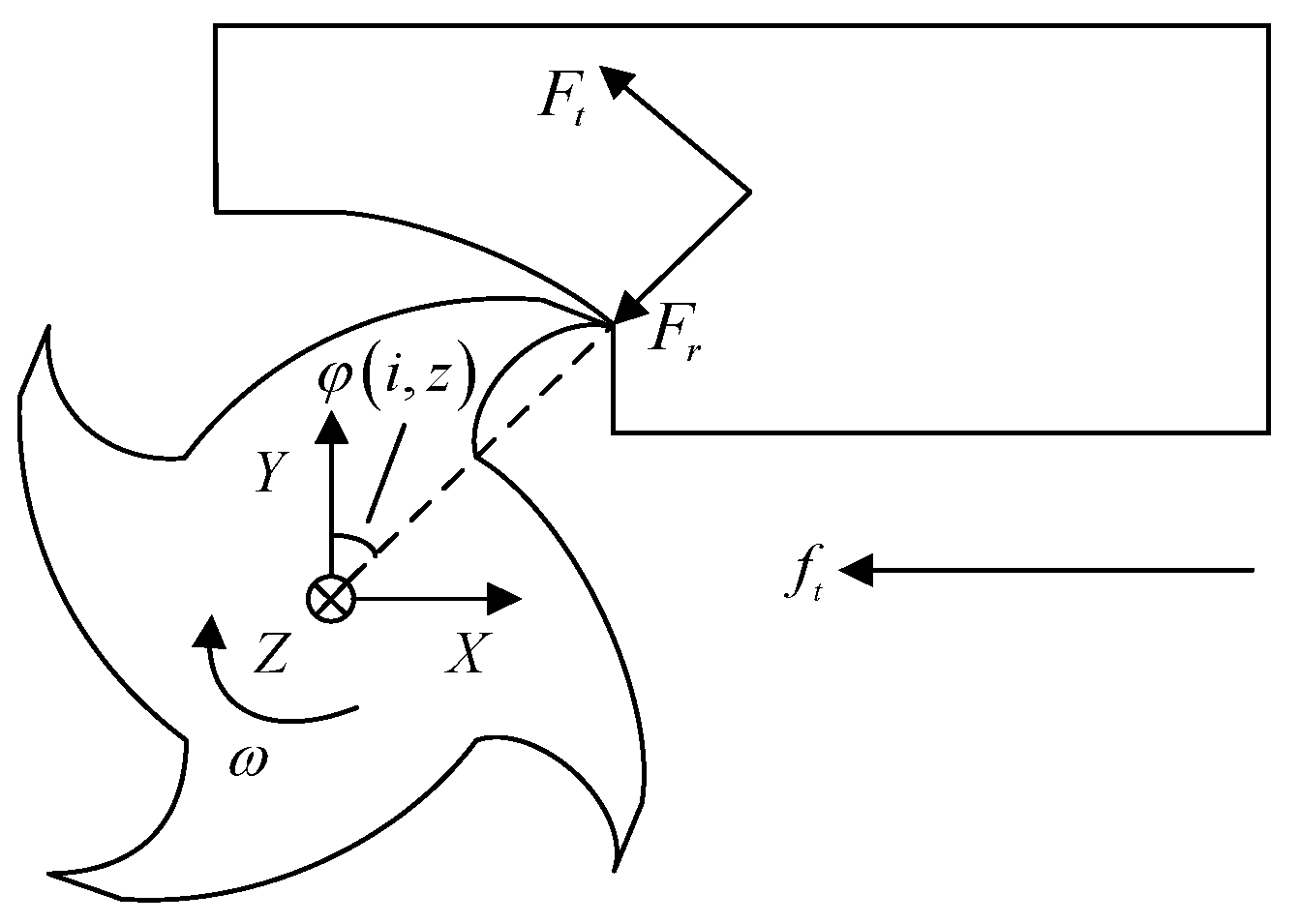
In order to establish the milling force prediction model of the variable helix end mill, force analysis was firstly carried out; the milling method was up-cut milling, and the established coordinate system is shown in Figure 6.

In order to facilitate the analysis, the micro-element milling force is usually converted into the workpiece coordinate system, and the transformation matrix can be obtained from the geometric relationship in Figure 6.

$$T_{i,z}=\left[\begin{array}{ccc}-\cos \left(\phi \left(i,z\right)\right)& -\sin \left(\phi \left(i,z\right)\right)& 0\\ \sin \left(\phi \left(i,z\right)\right)& -\cos \left(\phi \left(i,z\right)\right)& 0\\ 0& 0& 1\end{array}\right].$$

(9)

The micro-element milling force at the height z on the i-th cutting edge in the workpiece coordinate system can be written as:

$$d{F}_{i,z}=\left[\begin{array}{c}d{F}_x\\ d{F}_y\\ d{F}_z\end{array}\right]=T_{i,z}\left[\begin{array}{c}d{F}_t\\ d{F}_r\\ d{F}_a\end{array}\right].$$

(10)

In this paper, the average cutting force coefficient model was adopted, the milling force coefficient was regarded as a constant, and the milling force coefficient was calculated by the average milling force as follows:

$$\{\begin{array}{l}\overline{F_x}=-\frac{N{a}_p}{4}{K}_{rc}{f}_z-\frac{N{a}_p}{\pi }{K}_{re}\\ \overline{F_y}=\frac{N{a}_p}{4}{K}_{tc}{f}_z+\frac{N{a}_p}{\pi }{K}_{te}\\ \overline{F_z}=\frac{N{a}_p}{\pi }{K}_{ac}{f}_z+\frac{N{a}_p}{2}{K}_{ae}\end{array}.$$

(11)

A milling force coefficient discrimination experiment was designed and performed, using the slot milling method; the experimental parameters and the average milling force measurement results are shown in

Table 1. Milling force coefficient identification experimental data.

Experiment Number	Feed per Tooth (mm/z)	$\overline{{\mathit{F}}_{\mathbf{x}}}\left(\mathbf{N}\right)$	$\overline{{\mathit{F}}_{\mathbf{y}}}\left(\mathbf{N}\right)$	$\overline{{\mathit{F}}_{\mathbf{z}}}\left(\mathbf{N}\right)$
1	0.01	18.99	26.07	−0.24
2	0.02	32.13	34.81	−1.55
3	0.03	43.82	38.06	−2.95
4	0.04	56.07	42.87	−4.43
5	0.05	65.83	45.42	−6.19
6	0.06	76.27	46.12	−7.73

.

Taking the feed as the independent variable and the measured corresponding average milling force as the dependent variable, the linear regression equation between the average milling force and the feed was established by the least squares method. The identified milling force coefficients are shown in

Table 2. Milling force factor.

Shear Coefficient (N/mm2)	Value	Plow Force Coefficient (N/mm2)	Value
Ktc	870.04	Kte	38.01
Krc	−2284.21	Kre	−13.95
Kac	−245.87	Kae	1.66

.

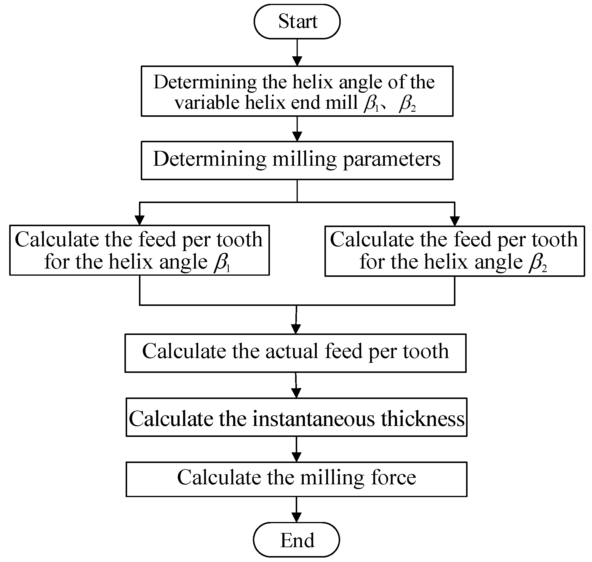
According to the theoretical model of the milling force, a MATLAB solution program was written to analyze the influence of the variable helical characteristics on the milling force. The solution process is shown in Figure 7.

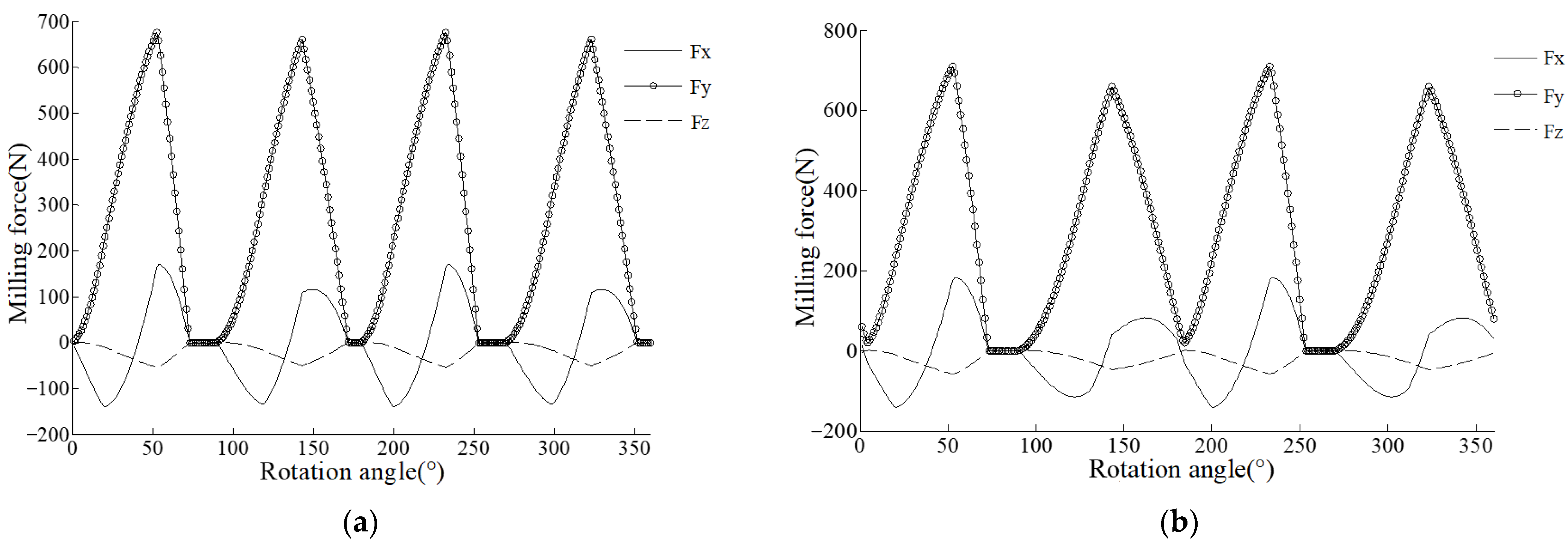
The selected milling parameters were a radial depth of cut of 2 mm and an axial depth of cut of 3 mm; the small helix angle blade entered the cutting first. Figure 8a,b show the plots of the milling force of the variable helix end mill with helix angles of [30°/40°] and [30°/50°].

It can be seen from Figure 8a that the cutting process maintains a single-tooth cutting state, the changing trend of the milling force of the cutting edges with different helix angles is the same, and the peak value of the milling force changes, among which the change in the milling force in the Z-direction is small. For the cutting edge with a larger helix angle, the peak values of the milling force in the X- and Y-directions are increased. Comparing the phase difference of two adjacent teeth, the phase difference during the rotation from the 30° cutting edge to the 40° cutting edge is greater than the rotation from the 40° cutting edge to the 30° cutting edge. This shows that the period of milling force changed due to the difference in pitch angle of adjacent cutting edges.

It can be seen from Figure 8b that, during the rotation of the 50° cutting edge to the 30° cutting edge, the two cutting edges participate in cutting at the same time. Therefore, for variable helix end mills, in addition to changing the axial depth of cut and radial depth of cut, the number of cutting edges involved in simultaneous cutting can be controlled by changing the size of the second helix angle. Comparing Figure 9 and Figure 10, it can be found that, when the second helix angle is larger, the variation range of the pitch angle increases, resulting in a change in peak milling force of the adjacent cutting edges in the three directions and a phase difference between the cutting edges.

3. Finite Element Simulation Analysis of Milling

Through the finite element simulation, the milling process of the variable helix end mill can be truly reflected. By modifying the finite element model and processing parameters, milling simulations under different working conditions were carried out, which allowed analyzing the influence of the variable helix angle structure on the milling force. Using ABAQUS software, a finite element model for milling titanium alloy with variable helix end mill was established, and the influence of different second helix angles on the milling force was analyzed.

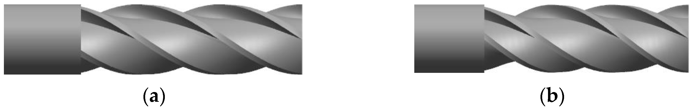
To simulate the milling process, a three-dimensional model of the helix angle of the [35°/38°] variable helix end mill was first established. In this paper, the curve winding method was used to construct the helical unfolding line first, and then the variable helix structure was obtained by winding. Figure 9 shows the three-dimensional models of end mills with different helix angle structures established using this method.

Comparing the two types of milling cutters with helical angle structures in Figure 9, the shape of the helical groove of the variable helical end mill was changed, and the pitch and phase at different axial heights were different from those of the standard milling cutter.

The diameter of the variable helix end mill used in the simulation was 10 mm, the number of teeth was 4, the total length of the milling cutter was 75 mm, and the effective length of the blade was 30 mm. Carbide was selected as the milling cutter material, and its physical properties are shown in

Table 3. Physical properties of cemented carbide materials.

Density	Young’s Modulus	Poisson’s Ratio	Specific Heat Capacity	Heat Transfer Coefficient
1.44 g/cm3	640 GPa	0.22	220 J/(kg·°C)	75.4 W/(m·K)

.

The workpiece material used in the simulation was Ti6Al4V, and its physical properties are shown in

Table 4. Physical properties of Ti6Al4V material.

Density	Young’s Modulus	Poisson’s Ratio	Yield Strength	Shear Strength	Heat Transfer Coefficient
4.44 g/cm3	108 GPa	0.34	870 MPa	760 MPa	0.9

.

In order to express the stress–strain relationship of the material and reflect its superelasticity and nonlinearity, scholars have established a constitutive model. At present, there are many kinds of constitutive models. Ti6Al4V is subjected to the action of milling force and cutting heat during the milling process, resulting in a large elastic–plastic strain. Therefore, this tudy adopted the Jonson–Cook constitutive model to simulate the stress–strain relationship of Ti6Al4V in the milling process. The expression for this model can be written as follows [29]:

$$\sigma =(\mathrm{A}+\mathrm{B}\cdot {\epsilon }^n\left)\right(1+\mathrm{C}\cdot \mathrm{In}(\frac{\stackrel{•}{\epsilon }}{{\stackrel{•}{\epsilon }}_0}\left)\right)(1-{\left(\frac{T-T_r}{T_m-T_r}\right)}^m),$$

(12)

where A, B, C, m, and n are material constants, T is the parameter temperature, T_m is the melting point temperature of the material, T_r is the room temperature, ε is the equivalent plastic strain, $\dot{\epsilon }$ is the equivalent plastic strain rate, and ${\dot{\epsilon }}_0$ is the reference strain rate. The corresponding JC constitutive model data are shown in

Table 5. JC constitutive model data of Ti6Al4V material [30].

A	B	C	n	m	Tm	Tr
860 MPa	683 MPa	0.035	0.47	1	1560 °C	20 °C

.

Milling is a process of continuously removing material, which is reflected in the finite element simulation as the deformation failure of the cut element, and the failed element is deleted. Since the JC constitutive model is used, the corresponding failure and separation criteria use the Jonson–Cook damage evolution model. The principle of this model is to set incremental steps through the iterative convergence of finite element software to perform damage evolution on mesh elements. When the element’s damage parameter ω is >1, the element fails and is deleted. The calculation formula of the damage parameter ω can be written as:

$$\omega =\frac{{\overline{\epsilon }}_0^{pl}+{\displaystyle \sum {\overline{\epsilon }}_{}^{pl}}}{{\overline{\epsilon }}_f^{pl}},$$

(13)

where $\overline{{\epsilon }_0^{pl}}$ is the initial value of the equivalent plastic strain, $\overline{{\epsilon }^{pl}}$ is the equivalent plastic strain increment, and $\overline{{\epsilon }_f^{pl}}$ is the failure strain. The failure strain formula defined by the Jonson–Cook damage evolution model can be written as:

$${\overline{\epsilon }}_f^{pl}=(d_1+d_2\exp (d_3\frac{p}{q}))(1+d_{4}In(\frac{\stackrel{•}{\epsilon }}{{\stackrel{•}{\epsilon }}_0}))(1+d_5(\frac{T-T_r}{T_m-T_r})),$$

(14)

where d₁, d₂, d₃, d₄, and d₅ are material failure parameters, p is the compressive stress, and q is the von Mises stress. The failure parameters of Ti6Al4V material are shown in

Table 6. Failure parameters of Ti6Al4V material [30].

Material	d1	d2	d3	d4	d5
Ti6Al4V	−0.09	0.25	−0.5	0.014	3.87

.

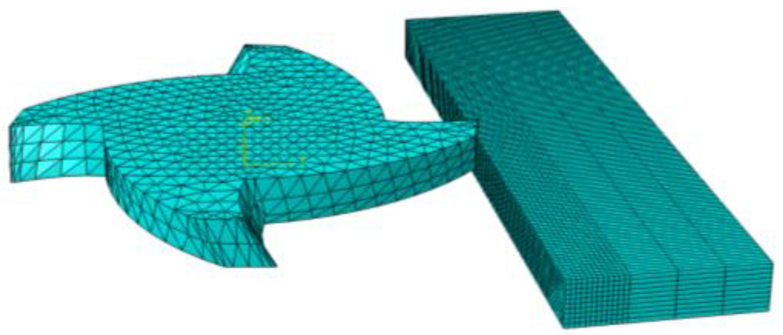
The meshing is shown in Figure 10. Since the structure of the tool was relatively complex, the tool mesh was divided using a free division method, and the overall mesh was a tetrahedral element. In order to reduce the amount of calculation and improve the calculation accuracy, when dividing the workpiece unit, the milling area and the non-milling area were divided. The milling area used small units, and the division was denser, whereas the non-milling area used large units, and the division was relatively sparse.

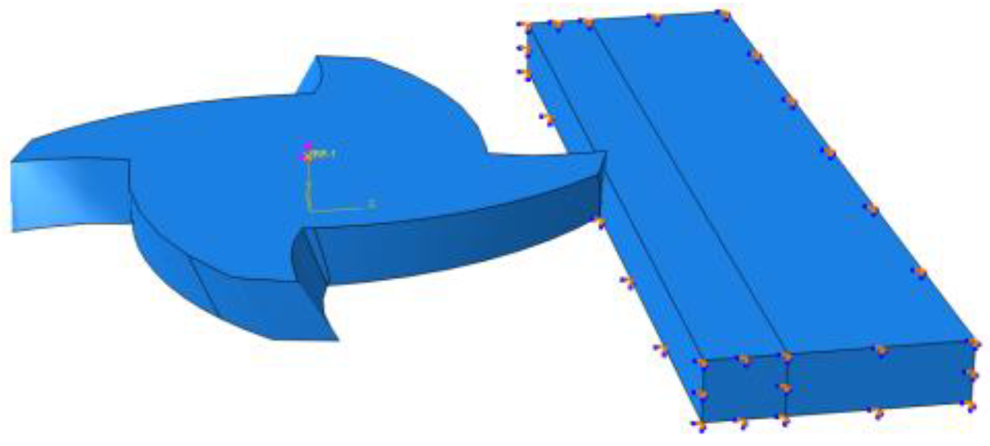
The machining conditions in the actual machining were reflected in the load settings in the finite element simulation. Except for the contact surface with the tool, the other planes on the workpiece could be set as completely fixed constraints by applying boundary conditions. In order to facilitate the output of the simulation results of the milling force, a reference point was set at the top of the tool. Since the milling cutter was a rigid body in the model, the reference point of the tool could represent the entire milling cutter. The speed and feed of the tool were applied by applying loads to the reference point. When setting the reference point, attention was paid to coupling all mesh nodes of the tool model, such that the motion of the reference point could represent the motion of the rigid tool, with the load settings shown in Figure 11.

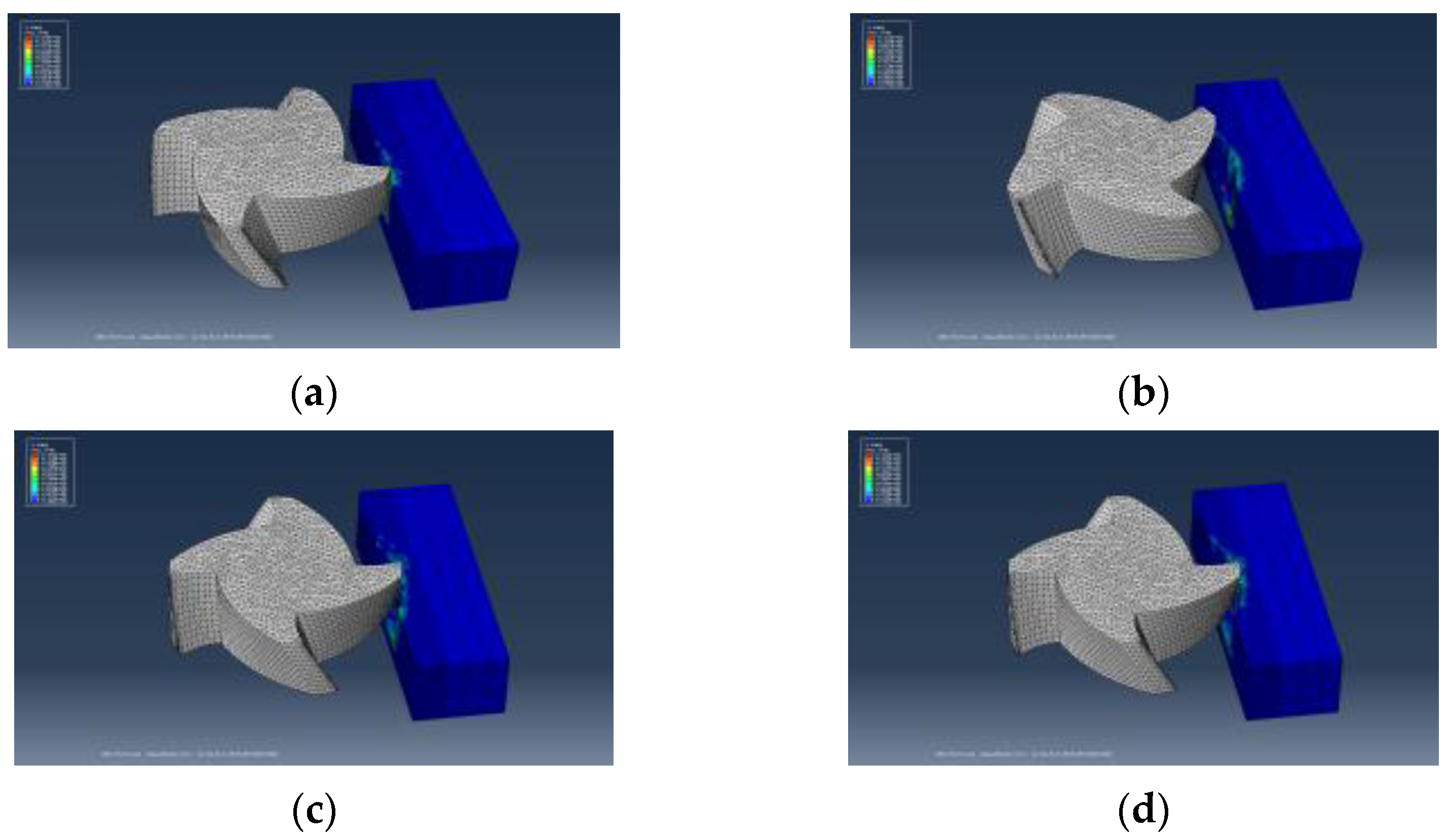
The set parameters were a spindle speed of 1200 r/min, a feed rate of 480 mm/min, and an axial depth of cut of 0.5 mm; the simulation process is shown in Figure 12.

Keeping the rake angle of the tool at 10°, the relief angle at 10°, and the first helix angle at 30°, the 3D model of the milling cutter with the second helix angles of 32°, 34°, 36°, and 38° was established for simulation. The obtained milling force peaks in all directions are shown in

Table 7. The second helix angle simulation results.

The Second Helix Angle	$\overline{{\mathit{F}}_{\mathbf{x}}}\left(\mathbf{N}\right)$	$\overline{{\mathit{F}}_{\mathbf{y}}}\left(\mathbf{N}\right)$	$\overline{{\mathit{F}}_{\mathbf{z}}}\left(\mathbf{N}\right)$	$\overline{\mathit{F}}\left(\mathbf{N}\right)$
30°	94.82	84.47	−12.68	127.62
32°	95.46	85.18	−13.33	128.63
34°	96.55	86.92	−14.17	130.68
36°	98.75	88.66	−14.61	133.51
38°	100.04	91.35	−16.77	136.51

.

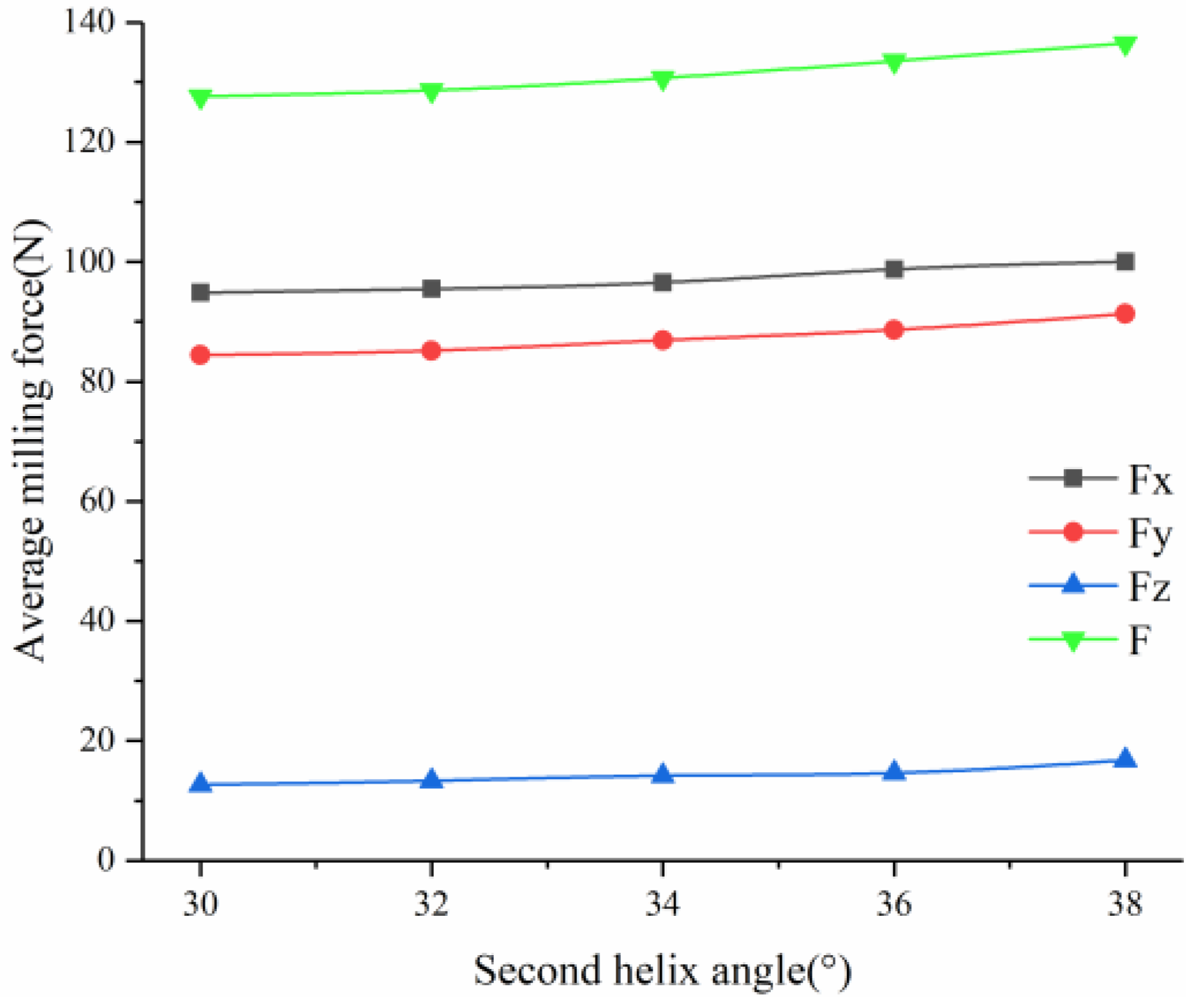
A line chart was plotted on the basis of the data in Table 7, as shown in Figure 13.

It can be seen from the analysis of the curve that, with the increase in the second helix angle, the overall average milling force increased gradually, the milling force in the X- and Y-directions increased greatly, and the milling force in the Z-direction increased slightly. This is because, with the increase in the second helix angle, the contact area between the corresponding cutting edge and the workpiece increased, and, although the helix angles of the other two cutting edges remained unchanged, the overall cutting area tended to increase. Therefore, the milling force increased.

4. Milling Stability Analysis

In order to analyze the influence of the variable helix end mill on the stability of the milling system, this section combines the process damping effect to solve the critical axial depth of cut of the variable helix end mill milling system.

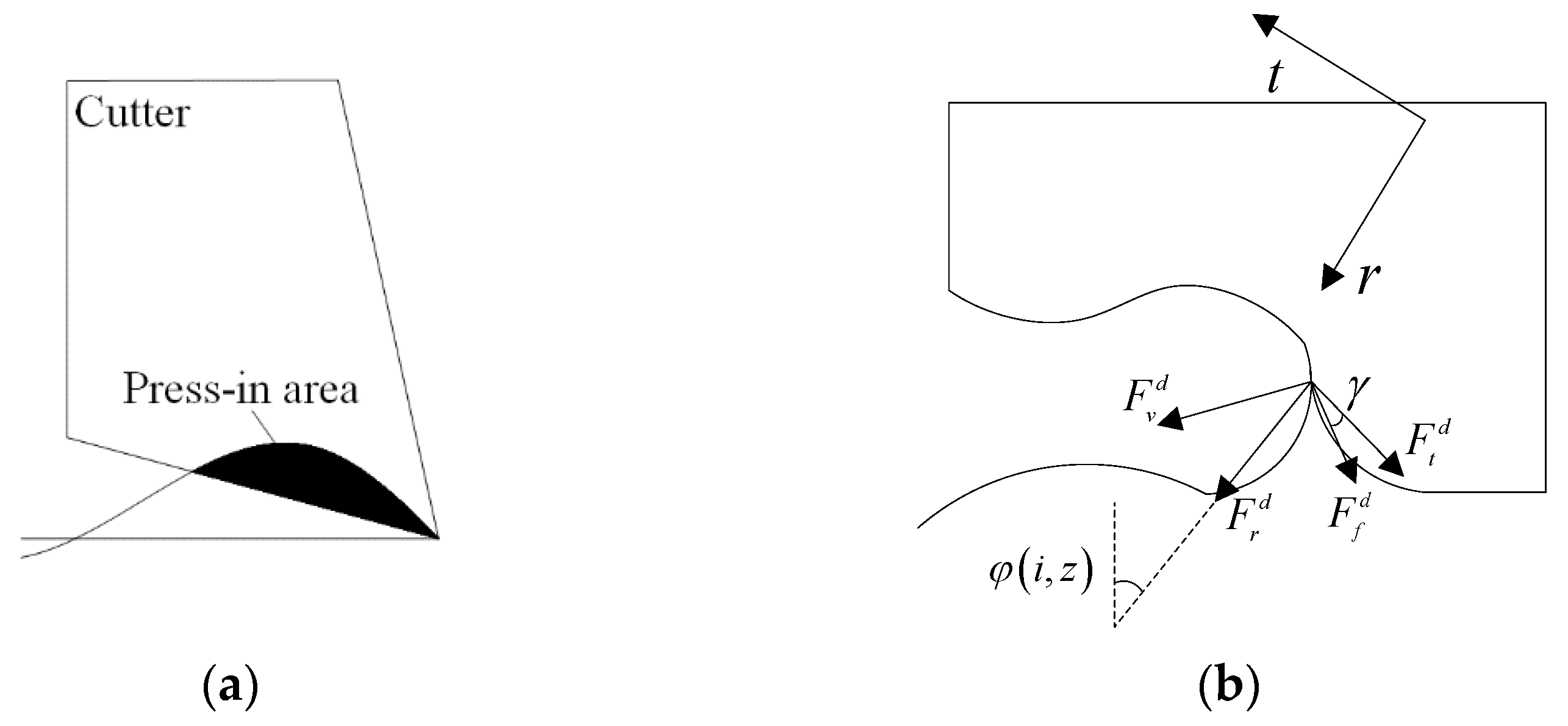
First of all, considering the occurrence of the process damping effect, during the milling process, due to the occurrence of vibration, the flank of the tool interferes with the vibration pattern on the surface of the workpiece, forming an indentation area as shown in Figure 14a.

When interference occurs, the schematic diagram of the force is as shown in Figure 14b. In the figure, $F_v^d$ is the pressing force generated by the interference action, and $F_f^d$ is the friction force generated by the interference action. $F_r^d$ and $F_t^d$ are the radial force and tangential force converted into the corresponding process damping force in the tool coordinate system, which are obtained by coordinate transformation. First, the pressing area was calculated [31].

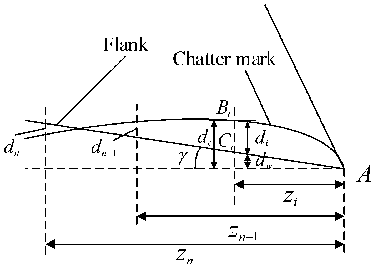
The schematic diagram of the pressing area when interference occurs is shown in Figure 15. In Figure 15, A is the contact point between the tool tip and the vibration pattern on the surface of the workpiece at the current moment. Taking the contact point as the starting point, the cutting edge is expanded in the circumferential direction. Then, take Δt as the time interval to discretize the time, let the arc length of two adjacent discrete points be Δs; then, Δs = v Δt, and let B_i be the vibration ripple point corresponding to each discrete timepoint, and C_i be the point on the flank face corresponding to the same timepoint. Let the vertical distance from point B_i to the circular development line be d_c, the vertical distance from point C_i to the circular development line be d_w, and the distance between B_i and C_i be d_i.

First, the radial coordinates of the vibration point and the corresponding point on the flank face can be solved as follows:

$$\{\begin{array}{cc}{z}_i=i\Delta s\hfill & i=1,2,\dots \\ d_c={\mathrm{z}}_i\tan (\gamma )\hfill & d_w=r-r_w\\ d_i=d_w-d_c\hfill & \end{array},$$

(15)

where r_w is the distance between the center axis of the tool and the vibration pattern point at the current moment, and the intersection of the flank face and the vibration pattern is determined by the step search method. Assuming that the intersection is located between the (n − 1)-th and n-th discrete timepoints, the search is performed along the flank face with Δt as the step, and the d_i value corresponding to each step is calculated in turn. When the value of d_n−1 is positive and the value of d_n is negative, it means that the intersection point is between the two points, and the search can be stopped. According to the obtained d_i values, the indentation area can be calculated as follows:

$$\{\begin{array}{l}\Delta A^i=\frac{d_i+d_{i+1}}{2}\Delta s\hspace{1em}i=2,\dots ,n-2\\ \Delta A^n=\frac{{(d_{n-1})}^2}{2(d_{n-1}-d_n)}\Delta s\hspace{1em}\Delta A^1=\frac{d_1\Delta s}{2}\\ U(t)={\displaystyle \sum _{i=1}^n\Delta A^i}\end{array}.$$

(16)

Similar to the calculation of the milling force, assuming that the process damping force F_d is proportional to the pressing area U, the micro-element process damping force can be written as:

$$\{\begin{array}{l}d{F}_v^d=K^{d}U(t,z)dz\\ d{F}_f^d=\mu d{F}_v^d\end{array},$$

(17)

where K^d is the indentation force coefficient, and μ is the friction coefficient. The indentation force coefficient can be calculated using Equation (18).

$$K^d=\frac{E}{1.29\rho (1-2\mu )},$$

(18)

where E is Young’s modulus, μ is Poisson’s ratio, and ρ is the degree of deformation, representing the distance of the elastic–plastic deformation zone during milling. This paper references the calibration results in [31]: K^d = 3 × 10⁴ N/mm³, μ = 0.3.

According to the geometric relationship shown in Figure 16, the micro-element process damping force of the tool coordinate system can be written as:

$$\{\begin{array}{l}d{F}_r^d=d{F}_v^d(\cos (\gamma )+\mu \sin (\gamma ))\\ d{F}_t^d=d{F}_v^d(-\sin (\gamma )+\mu \cos (\gamma ))\end{array}.$$

(19)

Combining Equations (8) and (19), the micro-element milling force considering the process damping effect can be written as:

$$\{\begin{array}{l}d{F}_t=K_{tc}h(i,z)dz+K_{te}\frac{dz}{\cos \beta }-d{F}_r^d\\ d{F}_r=K_{rc}h(i,z)dz+K_{re}\frac{dz}{\cos \beta }+d{F}_t^d\\ d{F}_a=K_{ac}h(i,z)dz+K_{ae}\frac{dz}{\cos \beta }\end{array}.$$

(20)

Equation (20) can be converted to the overall micro-element milling force in the workpiece coordinate system as follows:

$$\left[\begin{array}{c}d{F}_x\\ d{F}_y\\ d{F}_z\end{array}\right]=T\left[\begin{array}{c}d{F}_t\\ d{F}_r\\ d{F}_a\end{array}\right].$$

(21)

The solution of the vibration point coordinates affects the establishment of the dynamic equation; thus, under the condition of rigid workpiece, the coordinates of the new vibration point can be judged by the position of the cutting edge. Assuming that the mode shape function of the tool at different blade heights is Φ(z), then the instantaneous position of the blade whose height is z on the i-th tooth in the vibration state is as follows [32]:

$$\{\begin{array}{l}x(t)=R\sin \left(\phi \left(i,z\right)\right)+{\Phi }_x\left(z\right)x_{c,i}\\ y(t)=R\cos \left(\phi \left(i,z\right)\right)+{\Phi }_y\left(z\right)y_{c,i}\end{array},$$

(22)

where $\left(x_{c,I},y_{c,i}\right)$ is the vibration displacement of the tool during the machining process, and Φ_x(z) and Φ_y(z) are the mode shape functions in the X- and Y-directions of the tool.

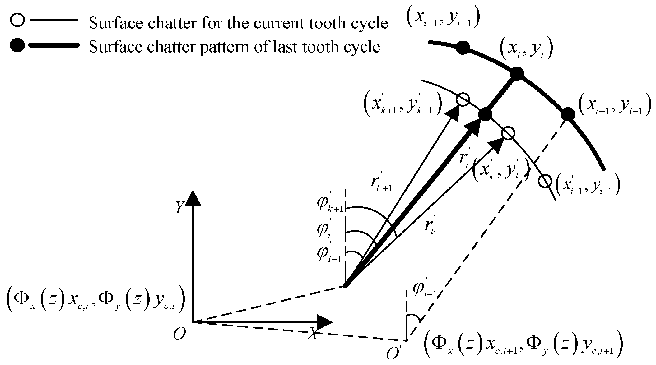
Figure 16 is a schematic diagram of the vibration pattern coordinates. For the surface vibration pattern point $\left(x_i,y_i\right)$ at the i-th timepoint, its source has the following two possibilities:

• If the tool is in the cutting state, the surface chatter point left is the same as the instantaneous position of the cutting edge;
• If the tool is in an uncut state, i.e., it is not in contact with the workpiece, then the surface vibration point at this time is the coordinate point left after the last cutting.

To determine which of the above cases is represented by $\left(x_i,y_i\right)$, it is necessary to find the surface vibration point $\acute{{\phi }_i}$ at the corresponding azimuth angle $\left(\acute{x_i},\acute{y_i}\right)$ in the previous cutting cycle, and calculate the distance ${\acute{r}}_i$ between this point and the central axis of the tool. The relationship between ${\acute{r}}_i$ and the tool radius can be compared to judge the cutting situation at this time.

After discretizing the cutting process into time elements, for an arbitrary timepoint i, we can search for two adjacent discrete timepoints k and k + 1 points at this moment. Assuming that the coordinates of the vibration pattern points corresponding to the two discrete timepoints are $\left(x_k^{\prime },y_k^{\prime }\right)$ and $\left(x_{k+1}^{\prime },y_{k+1}^{\prime }\right)$, the azimuth angles are ${\phi }_k^{\prime }$ and ${\phi }_{k+1}^{\prime }$, and the distances from the central axis of the tool are $r_k^{\prime }$ and $r_{k+1}^{\prime }$; these two distance values can be written as:

$$r_k^{\prime }=\sqrt{{\left(x_k^{\prime }-{\Phi }_x(z)x_{c,k}\right)}^2+{\left(y_k^{\prime }-{\Phi }_y(z)x_{c,k}\right)}^2},$$

(23)

$$r_{k+1}^{\prime }=\sqrt{{\left(x_{k+1}^{\prime }-{\Phi }_x(z)x_{c,k+1}\right)}^2+{\left(y_{k+1}^{\prime }-{\Phi }_y(z)x_{c,k+1}\right)}^2}.$$

(24)

Then, the azimuth corresponding to the two discrete points can be written as:

$${\phi }_k^{\prime }=\arcsin (\frac{y_k^{\prime }-{\Phi }_y(z)x_{c,k}}{r_k^{\prime }}),$$

(25)

$${\phi }_{k+1}^{\prime }=\arcsin (\frac{y_{k+1}^{\prime }-{\Phi }_y(z)x_{c,k+1}}{r_{k+1}^{\prime }}).$$

(26)

The search stop conditions are set to ${\phi }_k^{\prime }<{\phi }_i^{\prime }<{\phi }_{k+1}^{\prime }$. After the search is stopped, if the time element used is small enough, the coordinates of the adjacent vibration pattern points can be regarded as linear changes, and $r_i^{\prime }$ can be calculated by linear interpolation.

$$r_i^{\prime }=r_k^{\prime }+\frac{r_{k+1}^{\prime }-r_k^{\prime }}{{\phi }_{k+1}^{\prime }-{\phi }_k^{\prime }}\left({\phi }_i^{\prime }-{\phi }_k^{\prime }\right).$$

(27)

In this way, the instantaneous cutting thickness h can be written as

$$\{\begin{array}{ll}h=R-r_i^{\prime }& R>r_i^{\prime }\\ h=0& R<r_i^{\prime }\end{array}.$$

(28)

The coordinates of the surface vibration point of the workpiece in the previous cutting cycle can be written as:

$$\{\begin{array}{l}{x}_i^{\prime }=r_i^{\prime }\sin ({\phi }_i)+{\Phi }_x(z)x_{c,i}\\ y_i^{\prime }=r_i^{\prime }\cos ({\phi }_i)+{\Phi }_y(z)y_{c,i}\end{array}.$$

(29)

Then, the new workpiece surface vibration point coordinates can be written as:

$$\{\begin{array}{ll}\left(x_i,y_i\right)=(x(t),y(t))& R-r_i^{\prime }\ge 0\\ \left(x_i,y_i\right)=\left(x_i^{\prime },y_i^{\prime }\right)& R-r_i^{\prime }<0\end{array}.$$

(30)

Since the workpiece is continuously feeding, the tool coordinate system is also constantly moving; therefore, every time the tool rotates for a timestep Δt, f is the feed rate, and the surface vibration pattern coordinates of the workpiece must be updated, i.e., Δx is moved along the X axis.

$$\Delta x=-f\frac{\Delta t}{T}.$$

(31)

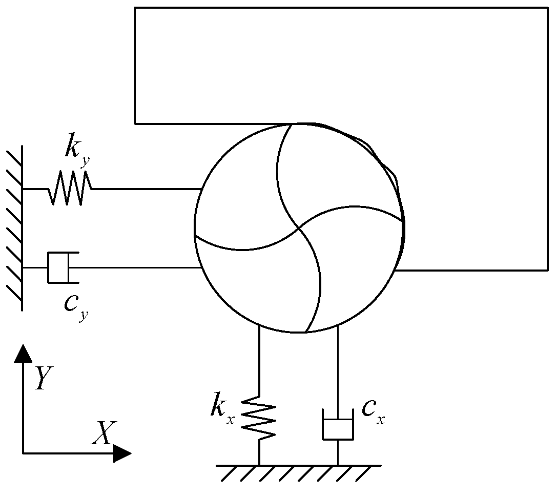
After completing the calculation of the relevant parameters, the dynamic equation can be established. Considering that the rigid workpiece does not vibrate, this section takes a spindle–tool system as the stability research object. In the specific machining process, the vibration of the entire system in the two degrees of freedom of feed (X-direction) and vertical direction (Y-direction) is analyzed, and it is simplified into a two-degree-of-freedom damped vibration system as shown in Figure 17.

If the modal coupling of the spindle–tool system is not considered, we can perform modal analysis in the X- and Y-directions respectively. Taking the modal analysis in the X-direction as an example, the milling cutter fixed on the spindle can be regarded as a cantilever beam, and the cutter is discretized into n micro-elements from the fixed end to the free end. Since these tool elements are identical in structure, the corresponding modal parameters (m_x, c_x, k_x) are exactly the same. The main difference is that the mode shape coefficients of each element are different, which is related to the position of the element in the Z-direction. We can set its mode shape coefficient as the Φ_x(z) function; then, the corresponding natural mode shape of a certain order mode is {Φ_x(z)}, and the mode shape coefficient of the tool tip position is assumed to be 1.

Then, according to the mass matrix [M_x], damping matrix [C_x], and stiffness matrix [K_x] of the system, the modal parameters in the X direction can be obtained as:

$$\{\begin{array}{l}{m}_x={\left\{{\Phi }_x\left(z\right)\right\}}^T\left[M_x\right]\left\{{\Phi }_x\left(z\right)\right\}\\ c_x={\left\{{\Phi }_x\left(z\right)\right\}}^T\left[C\right]\left\{{\Phi }_x\left(z\right)\right\}\\ k_x={\left\{{\Phi }_x\left(z\right)\right\}}^T\left[K_x\right]\left\{{\Phi }_x\left(z\right)\right\}\\ {\Phi }_x\left(0\right)=1\end{array}.$$

(32)

Similarly, the modal parameter (m_y, c_y, k_y, Φ_y(z)) in the Y-direction is consistent with that in the X-direction.

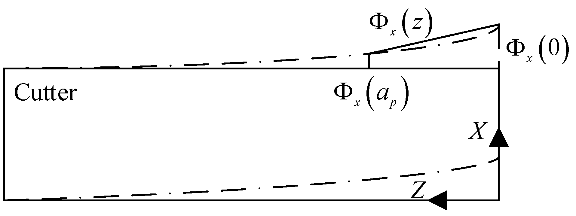
According to the principle of regenerative chatter vibration, the spindle–tool system is excited by the milling force in the X- and Y-directions, resulting in vibration in the corresponding directions. Assuming that the vibration displacement of the tool nose position is (x_c, y_c), the vibration displacement at any height is (x_c Φ_x(z), y_c Φ_y(z)), and the Φ(z) function can be solved by the interpolation method. Assuming that the mode shape coefficient changes linearly from the free end (z = 0) of the tool to the cutting end (z = a_p), the entire mode shape function can be obtained by identifying the mode shape coefficients of two points, as shown in Figure 18.

Considering the occurrence of regenerative chatter, the instantaneous cutting thickness of the cutting edge is divided into two parts: static cutting thickness $h_s\left({\phi }_j\right)$ and dynamic cutting thickness $h_d\left({\phi }_j\right)$.

$$h\left({\phi }_j\right)=h_s\left({\phi }_j\right)+h_d\left({\phi }_j\right).$$

(33)

According to the analytical expression of the milling force of the end mill, the static cutting thickness is related to the feed per tooth and the azimuth angle. Under the condition of rigid workpiece milling, the dynamic cutting thickness only considers the vibration of the tool, as shown in Figure 19.

Instantaneous cutting thickness $h\left({\phi }_j\right)$ can be written as:

$$h\left({\phi }_j\right)=\left[f_z\sin \left({\phi }_j\right)+\left(v_j\left(t-T\right)-v_j\left(t\right)\right)\right]g\left({\phi }_j\right)=\left[\begin{array}{l}{f}_z\sin \left({\phi }_j\right)-\left[\sin \left({\phi }_j\right)\cos \left({\phi }_j\right)\right]\\ \left\{\begin{array}{l}{\Phi }_x\left(z\right)\left[x_c\left(t\right)-x_c\left(t-T\right)\right]\\ {\Phi }_y\left(z\right)\left[y_c\left(t\right)-y_c\left(t-T\right)\right]\end{array}\right\}\end{array}\right]g\left({\phi }_j\right),$$

(34)

where ${\phi }_{st}$ is the cut-in angle of the cutting edge, ${\phi }_{ex}$ is the cut-out angle of the cutting edge, and the unit step function $g\left({\phi }_j\right)$ used to judge the cutting state of the cutting edge can be written as:

$$g\left({\phi }_j\right)=\{\begin{array}{l}1\hspace{1em}\hspace{1em}{\phi }_{st}<{\phi }_j<{\phi }_{ex}\\ 0\hspace{1em}{\phi }_j<{\phi }_{st}\mathrm{or}{\phi }_j>{\phi }_{ex}\end{array}.$$

(35)

In the workpiece coordinate system, the micro-element milling forces in the X- and Y-directions can be written as:

$$\left[\begin{array}{c}d{F}_{x,j}\\ d{F}_{y,j}\end{array}\right]=T_j\left[\begin{array}{l}{K}_{tc}{h}_j\left({\phi }_j\right)dz+K_{te}\frac{dz}{\cos \beta }-d{F}_r^d\\ K_{rc}{h}_j\left({\phi }_j\right)dz+K_{re}\frac{dz}{\cos \beta }+d{F}_t^d\end{array}\right],$$

(36)

where T_j is the transformation matrix from the tool coordinate system to the workpiece coordinate system, which can be written as:

$$T_j=\left[\begin{array}{cc}\cos \left({\phi }_j\right)& -\sin \left({\phi }_j\right)\\ \sin \left({\phi }_j\right)& \cos \left({\phi }_j\right)\end{array}\right].$$

(37)

Finally, the milling forces of all cutter teeth and all micro-elements can be superimposed to obtain the milling dynamics equation, which can be written as:

$$\{\begin{array}{l}{m}_x\stackrel{··}{x_c}+c_x\stackrel{·}{x_c}+k_x{x}_c={\displaystyle \sum _{j=1}^N{\displaystyle \sum _{k=1}^{S}g\left({\phi }_j\left(z\right)\right)}{\Phi }_x\left(z\right)d{F}_{x,j}}\\ m_y\stackrel{··}{y_c}+c_y\stackrel{·}{y_c}+k_y{y}_c={\displaystyle \sum _{j=1}^N{\displaystyle \sum _{k=1}^{S}g\left({\phi }_j\left(z\right)\right)}{\Phi }_y\left(z\right)d{F}_{y,j}}\end{array}.$$

(38)

The time-domain solution method can be used to numerically calculate Equation (38) to obtain the time domain data of the entire system, and then to judge the stability of the entire system. The classical fourth-order Runge–Kutta method can be selected to solve the dynamic equations. First, according to the requirements of the Runge–Kutta method, the corresponding first-order differential equation can be established as follows:

$$y^{\prime }=f\left(t,y\right).$$

(39)

The milling dynamics equation can be rewritten into a new equation system, and the new function variable can be set as:

$$y={\left[x_c{y}_c\stackrel{·}{x_c}\stackrel{·}{y_c}\right]}^T.$$

(40)

The rewritten kinetic equations can be written as:

$$\{\begin{array}{l}\stackrel{·}{x}=\stackrel{·}{x}\\ \stackrel{·}{y}=\stackrel{·}{y}\\ -{\omega }_x^{2}x-2{\zeta }_x{\omega }_x\stackrel{·}{x}+F_x\left(t\right)/m_x=\stackrel{··}{x}\\ -{\omega }_y^{2}y-2{\zeta }_y{\omega }_y\stackrel{·}{y}+F_y\left(t\right)/m_y=\stackrel{··}{y}\end{array}.$$

(41)

The equation system in Equation (41) can be rewritten into a matrix form with Equation (40) as the function variable.

$$f=\left[\begin{array}{cc}\left[0\right]& \left[I\right]\\ \left[-{\omega }^2\right]& \left[-2\zeta \omega \right]\end{array}\right]y+\left[\begin{array}{c}\left[0\right]\\ \left[F\left(t\right)\right]\end{array}\right].$$

(42)

Each coefficient matrix in Equation (42) can be written as:

$$\left[-{\omega }^2\right]=\left[\begin{array}{l}-{\omega }_x^{2}0\\ 0-{\omega }_y^2\end{array}\right]=\left[\begin{array}{l}-k_x/m_{x}0\\ 0-k_y/m_y\end{array}\right],$$

(43)

$$\left[-2\zeta \omega \right]=\left[\begin{array}{l}-2\zeta {\omega }_{x}0\\ 0-2\zeta {\omega }_y\end{array}\right]=\left[\begin{array}{l}-c_x/m_{x}0\\ 0-c_y/m_y\end{array}\right],$$

(44)

$$\left[F\right]={\displaystyle \sum _1^{S}g\left({\phi }_j\left(z\right)\right)}\left[\begin{array}{l}{\Phi }_x\left(z\right)d{F}_{x,j}/m_x\\ {\Phi }_y\left(z\right)d{F}_{y,j}/m_y\end{array}\right]dz.$$

(45)

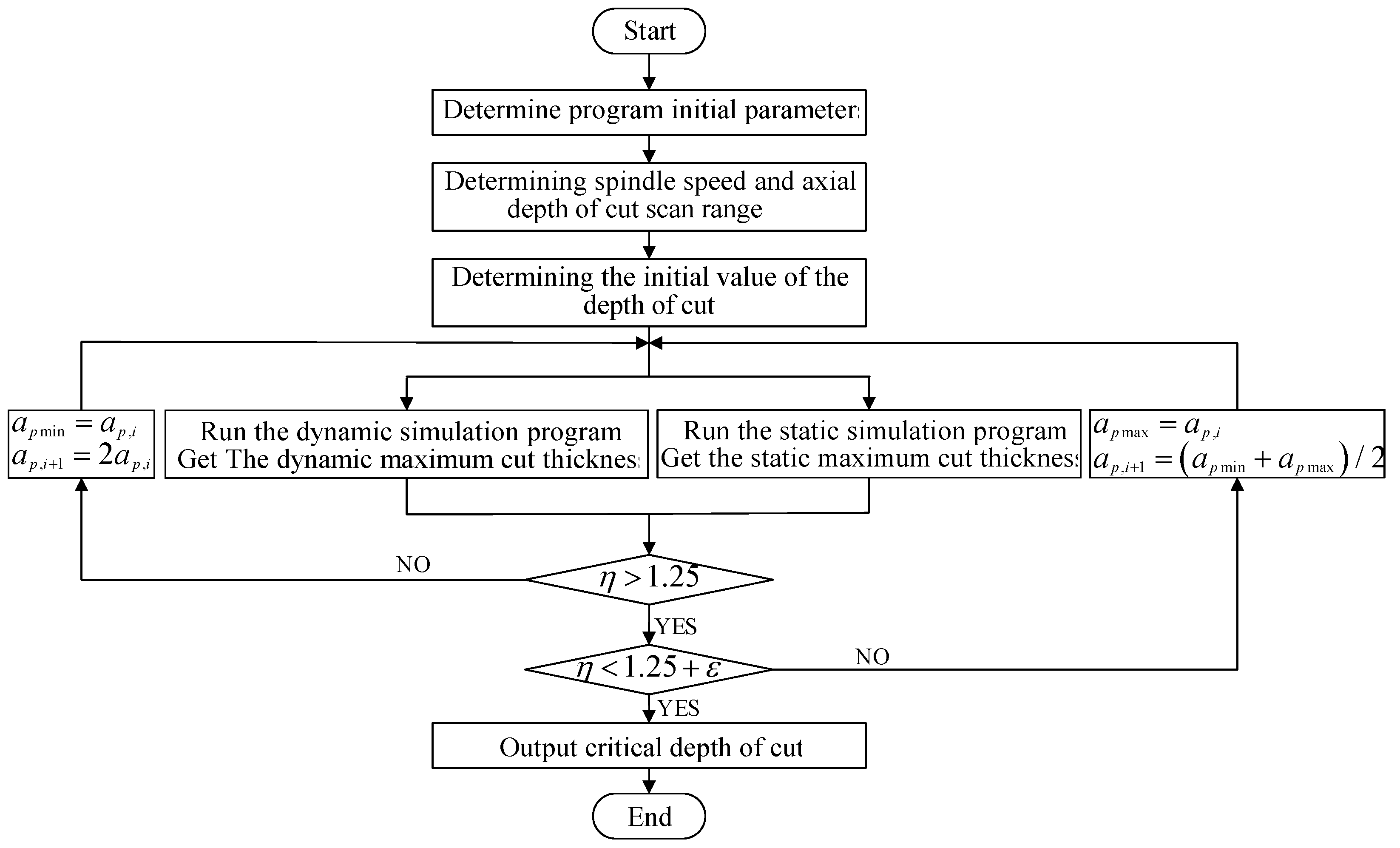
In order to reduce the amount of computation, the dynamic simulation time limit is set to two milling cycles, and the static simulation time is set to one milling cycle. According to the calculation rule of Runge–Kutta method, the recursive formula of the state quantity from the i-th timepoint to the (i + 1)-th timepoint can be obtained as:

$$\{\begin{array}{l}{y}_{i+1}=y_i+h\left(k_1+2k_2+2k_3+k_4\right)/6\\ k_1=f\left(t_i,y_i\right)\\ k_2=f\left(t_i+h/2,y_i+h{k}_1/2\right)\\ k_3=f\left(t_i+h/2,y_i+h{k}_2/2\right)\\ k_4=f\left(t_i+h,y_i+h{k}_3\right)\end{array}.$$

(46)

Unlike the solution method in the frequency domain, the time-domain method uses the ratio η of the maximum cutting thickness in the dynamic and static simulation as the basis for the occurrence of chatter.

$$\eta =\frac{h_{d,max}}{h_{s,max}},$$

(47)

where h_d,max is the maximum cutting thickness calculated by the dynamic simulation program, and h_s,max is the maximum cutting thickness calculated by the static simulation program. Due to the variable helix angle structure of the tool, the cutting thickness of the cutting edge at different heights is different. Here, the maximum cutting thickness of all micro-elements in the whole simulation cycle was selected.

The specific flow of flutter stability time-domain analysis is shown in Figure 20.

In this experiment, the influence of the blade height on the tool vibration was ignored. Therefore, it was assumed that the vibration conditions of the micro-element cutting edge at different heights were the same within the range of the axial cutting depth.

The time-domain method was used for the stability analysis of the milling system. Therefore, parameters such as modal mass (m_x, m_y), modal damping (c_x, c_y), and modal stiffness (k_x, k_y) needed to be obtained through experiments, and the modal parameters of the spindle–tool system were obtained through modal experiments as shown in

Table 8. Spindle–tool system modal parameters.

Modal Order	Natural Frequency (Hz)	Damping Ratio (%)	Modal Mass (kg)
X-direction first order	1493	3.885	4.41
X-direction second order	4253	1.105	1.39
Y-direction first order	1460	4.144	4.90
Y-direction second order	4280	1.646	1.81

.

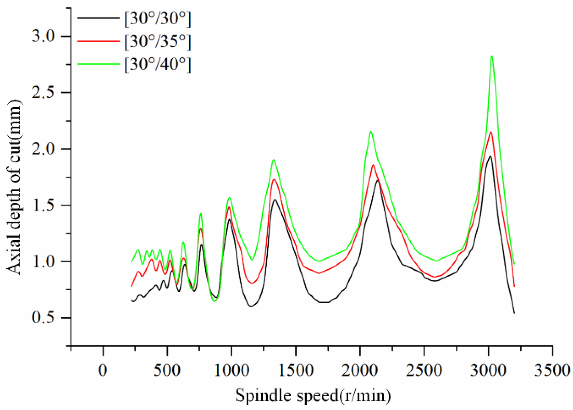
In order to analyze the influence of the variable helix angle structure on the milling stability, the milling stability lobe diagrams with variable helix angle parameters of [30°/30°], [30°/35°], and [30°/40°] were plotted, as shown in Figure 21.

Observing the images, it can be found that, on the whole, with the increase in the second helix angle, the maximum and minimum critical axial depths of cut increased, and the milling stability region showed an expanding trend. This may have been due to the change in the second helix angle, whereby the time delay range between adjacent cutting edges increased, which had a better suppression effect on chatter. There was no significant change in the minimum critical depth of cut between 750 and 1000 r/min. The reason may be that the increase in the helix angle led to an increase in the milling force, which affected the vibration weakening effect. Observing the images between 2000 and 3200 r/min, it can be found that, after the second helix angle changed, the spindle speed corresponding to the maximum critical depth of cut also changed.

5. Milling Experiment

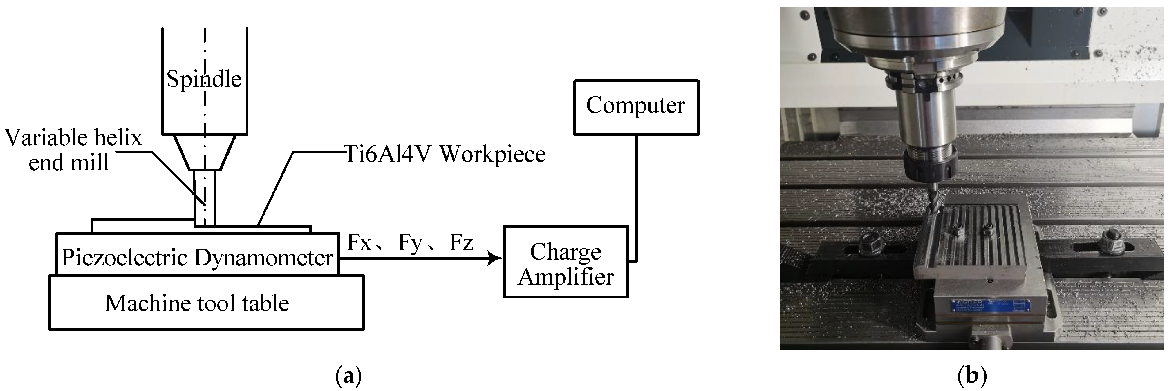
In order to analyze the application of variable helix end mills in actual machining, milling experiments were designed. As shown in Figure 22, the experimental equipment included a three-axis vertical machining center, piezoelectric force measuring instrument, charge amplifier, and optical digital microscope. A total of three experimental tools were selected, namely, 35° standard end mills and [30°/32°] and [35°/38°] variable helix end mills.

The roughness measurement equipment was a DSX510 optical digital microscope from OLYMPUS, as shown in Figure 23. During the measurement, five different points were selected on the surface of the workpiece, and the three-dimensional image of the surface was obtained by using the 3D acquisition mode. Using the surface roughness calculation module in the software, the average value of the five points was taken as the surface roughness value.

The milling force measurement system was a Swiss Kistler9257B piezoelectric force measuring instrument, as shown in Figure 24a; a Kistler5070 charge amplifier and acquisition card, as shown in Figure 24b, were also used, in conjunction with Dynoware computer analysis software.

The experimental equipment connection and milling experiments are shown in Figure 25a,b.

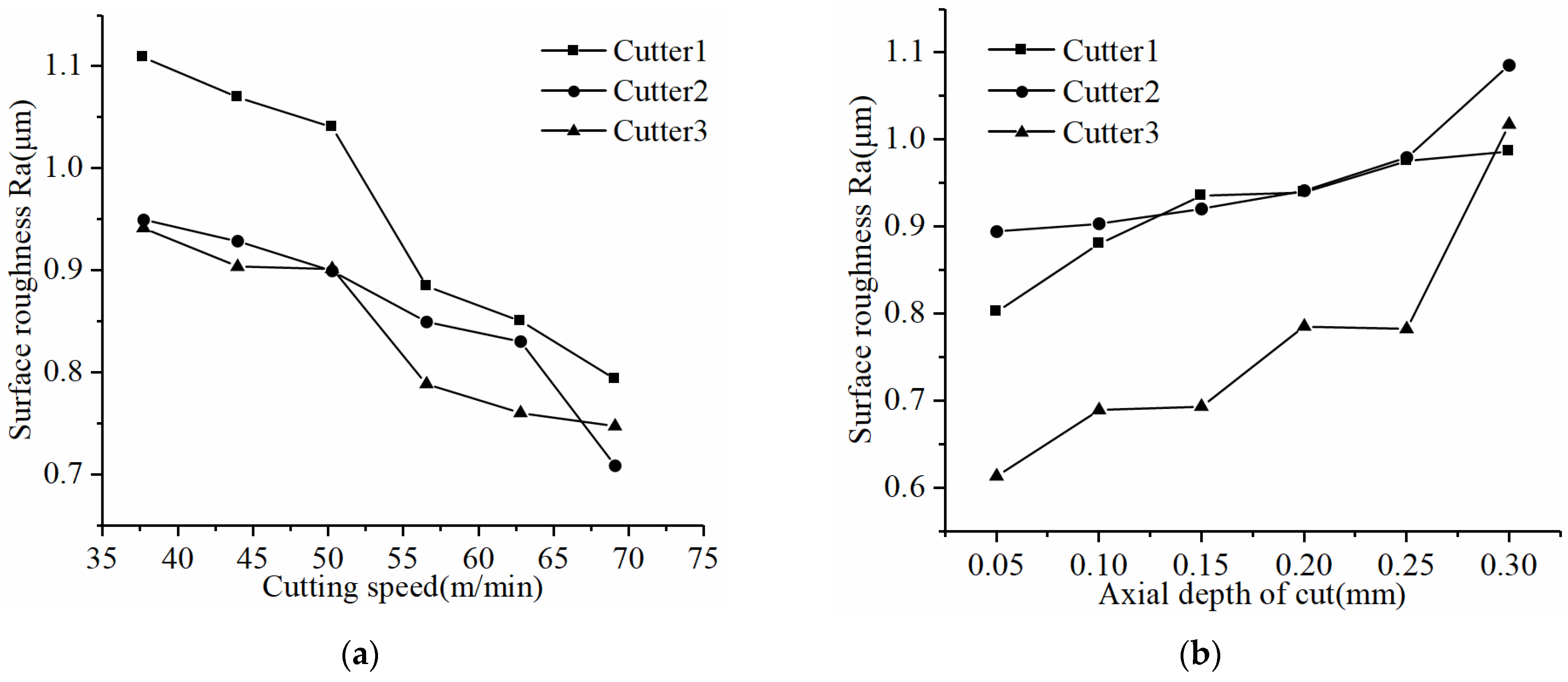
First, a single-factor milling experiment was carried out. The experimental factors were cutting speed and axial depth of cut. The surface roughness after machining was measured, and the curve was plotted as shown in Figure 26. In the figure, tool 1 is the [30°/32°] variable helix end mill, tool 2 is the 35° standard end mill, and tool 3 is the [35°/38°] variable helix end mill.

It can be seen from Figure 26 that, for the three tools in the experiment, with the increase in the cutting speed, the machined surface roughness of tool 1 and tool 2 showed a decreasing trend. The machined surface roughness of tool 3 showed a trend of decreasing first, then increasing, and finally decreasing. The main reason is that, with the increase in cutting speed, the machining time of the milling area was shortened, and the degree of plastic deformation in the area was weakened, thereby improving the surface roughness. As the axial depth of cut increased, the machined surface roughness also increased. This is because, with the increase in the axial depth of cut, the cutting area increased, the cutting force also increased, the stability of the milling system decreased, and the machined surface roughness increased.

Comparing the machining quality of the tools, the machining quality of tool 2 and tool 3 was generally higher than that of tool 1, which shows that the variable helix angle structure could suppress the vibration during the milling process. However, as the axial depth of cut increased, the machining quality of tool 2 became similar to or even slightly lower than that of tool 1. This shows that, within the range of the specified axial depth of cut, although tool 2 had a variable helix angle structure, due to the larger helix angle of tool 1, the contact area between the workpiece and the tool increased. Thus, chip removal was promoted, and the improvement effect on the machining quality was more obvious.

A four-factor and four-level orthogonal milling experiment was designed, and the average milling force was orthogonally analyzed. The four factors of cutting speed, feed per tooth, axial depth of cut, and radial depth of cut are represented by A, B, C, and D, respectively, and the range and variance analyses of the experimental results are shown in

Table 9. Range analysis table.

	Factor	A	B	C	D
Level
I		8.329	7.188	3.133	6.746
II		7.810	7.365	6.032	7.061
III		7.612	8.176	9.964	8.22
IV		7.267	8.288	11.887	8.991
Range		1.062	1.1	8.756	2.245
Effects from major to minor		C, D, B, A

and

Table 10. Variance analysis table.

Source	Degrees of Freedom	Seq SS	Adj SS	Adj MS	F	Salience
Cutting speed	3	2.365	2.365	0.788	17.77	0.05
Feed per tooth	3	3.741	3.741	1.247	28.11	0.05
Axial depth of cut	3	185.20	185.20	61.734	1391.6	0.05
Radial depth of cut	3	12.975	12.975	4.325	97.49	0.05
Error	3	0.133	0.133	0.044
Total	15	204.7762

.

It can be seen from the above analysis that the degree of influence on the milling force of the variable helix end mill was in the order axial depth of cut > radial depth of cut > feed per tooth > cutting speed. In terms of significance, the axial depth of cut had the greatest influence on the milling force.

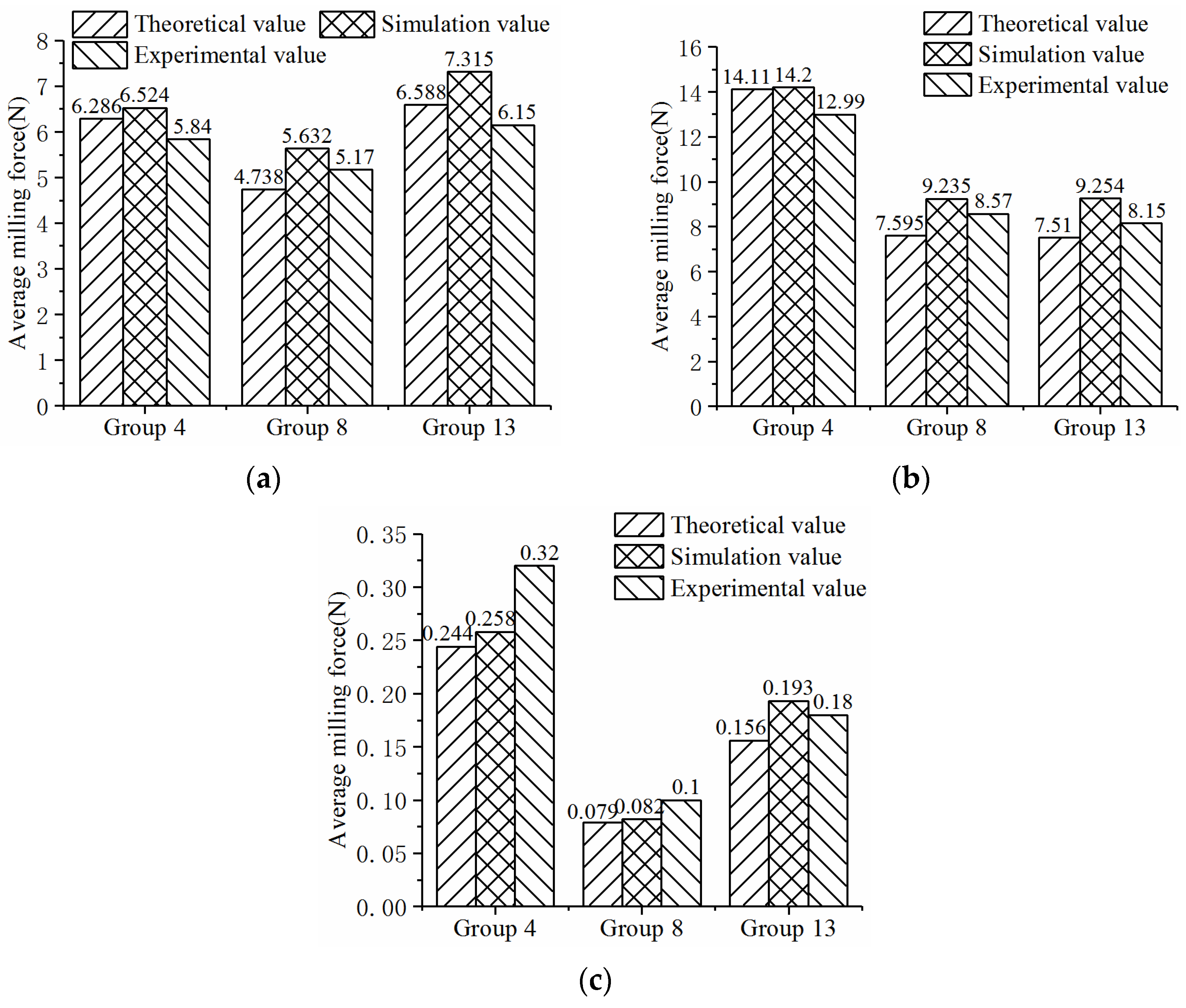
The three sets of orthogonal experimental results were used to verify the accuracy of the milling force prediction model and the finite element simulation model, and a comparison bar chart was drawn, as shown in Figure 27.

From Figure 27, it can be intuitively seen that there were differences between the average milling forces obtained in the three directions using different methods. The next step was to calculate the relative errors between the theoretical model and finite element model and the experimental data to evaluate the accuracy of the two models. The specific results are shown in

Table 11. Theoretical model milling force verification results.

Group	Milling Force Direction	Theoretical Value (N)	Experimental Value (N)	Relative Error (%)
4	X	−6.286	−5.84	7.64
	Y	14.11	12.99	8.62
	Z	−0.244	−0.32	23.8
8	X	−4.738	−5.17	8.4
	Y	7.595	8.57	11.4
	Z	−0.079	−0.1	21
12	X	−6.588	−6.15	7.12
	Y	7.51	8.15	7.85
	Z	0.156	0.18	13.3

and

Table 12. Milling force verification results of finite element simulation model.

Group	Milling Force Direction	Simulation Value (N)	Experimental Value (N)	Relative Error (%)
4	X	−6.524	−5.84	11.7
	Y	14.20	12.99	9.31
	Z	−0.258	−0.32	19.4
8	X	−5.632	−5.17	8.94
	Y	9.235	8.57	7.76
	Z	−0.082	−0.1	18
12	X	−7.315	−6.15	18.9
	Y	9.254	8.15	13.6
	Z	0.156	0.18	13.3

.

It can be seen from Table 11 that the relative error range between the milling force of the variable helix end mill calculated according to the theoretical model and the milling force measured by the milling experiment was 7.12–23.8%. It can be seen from Table 12 that the relative error range between the simulated milling force and the experimental milling force was 7.22–19.4%.

Through analysis, it can be found that the error may have been due to a certain simplification in the theoretical model, as the finite element simulation model assumed that the tool was a rigid body with a certain number of meshes. From the perspective of the overall error, the established variable helical milling cutter milling force prediction model and finite element simulation model have certain reference value for actual milling machining.

6. Conclusions

This paper explored the influence of the variable helix angle structure on the feed per tooth and cutting thickness, established the milling force theory and a finite element simulation model of the variable helix end mill, and analyzed the milling stability of the variable helix end mill. Finally, a milling experiment was designed to verify the model. The conclusions of the research are as follows:

(1)

The change trend of the feed per tooth of the adjacent cutting edges of the variable helix end mill is opposite, the change speed is the same, and the change speed increases with the increase in the second helix angle. The cutting thickness of the small teeth first increases and then decreases, the peak value moves in the direction of the greater height of the milling cutter with the increase in the second helix angle, and the cutting thickness of the cutting edge with a large helix angle decreases monotonically.

(2)

The peak value of the milling force of the variable helix end mill and the phase difference of the adjacent cutting edge curves are changed, and the peak value of the milling force of the cutting edge with a small helix angle is larger than that of the cutting edge. By adjusting the size of the second helix angle, the number of cutting edges participating in cutting at the same time can be changed. With the increase in the second helix angle, the average milling force in the X- and Y-directions increases, and the average milling force in the Z-direction increases slightly.

(3)

The variable helix end mill can increase the stability area of milling. When the second helix angle changes, the spindle speed corresponding to the maximum critical axial depth of cut in the high-speed area changes. Variable helix end mills can improve the surface quality to a certain extent.

(4)

The order of influence of each parameter on the milling force of the variable helical milling cutter was as follows: axial depth of cut > radial depth of cut > feed per tooth > cutting speed. The relative error range between the theoretical milling force and the experimental milling force was 7.12–23.8%, and the relative error range between the simulated milling force and the experimental milling force was 7.22–19.4%.