Abstract
Advanced cascade design theories and methods are crucial to the rapid development of torque converters. Therefore, the study proposed a new parametric design method for a hydrodynamic torque converter cascade. The method is embodied by using a cubic non-uniform rational B-splines (NURBS) open curve and closed curve, respectively, to carry out the parametric design of the unit blade camberline and unit blade thickness distribution, and the curvature of the designed blade curve is continuous. Then, the author developed batch and script files in the Isight platform for a fully automated integrated design of the hydrodynamic torque converter, including cascade parametric modeling, meshing, computational fluid dynamics (CFD) simulation, post-processing, and optimization design. A three-dimensional cascade integrated optimization design system of the hydrodynamic torque converter is established with CFD technology as the bottom layer design, a control file as the middle layer, and an optimization algorithm as the top layer drive. Finally, multi-objective optimization was carried out for the key cascade parameters (camberline peak height). Compared with the original blade, the optimized NURBS blade increased by 7.207% in high-efficiency region width (Gη), and the optimized blade increased by 2.673% in peak efficiency (ηmax) to meet the actual engineering requirements. The new parametric design method of the blade shape and the integrated optimization design system of a three-dimensional cascade of torque converter proposed in this paper significantly reduces the design costs and shortens the design cycle of the torque converter, which will provide a valuable reference for engineers of turbomachinery.
1. Introduction
The hydrodynamic torque converter is a power transmission device that realizes power transmission through energy conversion between a cascade and a transmission medium. The typical torque converter is composed of a radially installed pump (the pump shroud is connected to the engine, and the pump shroud is fixedly connected to the pump with hexagon bolts), a turbine (the turbine is directly connected to the input shaft of the gearbox), and an axially installed stator (the stator is fixed on the stationary hub) (Figure 1). Torque converters have good launching performance at low-speed ratios, a continuously variable torque, torque multiplication, and vibration isolation and are widely used in automobiles and construction machinery.
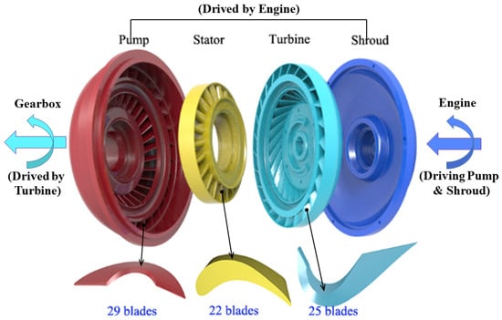
Figure 1.
Illustration of a torque converter.
In the past, constrained by developments in technology, Eulerian one-dimensional flow beam theory has become the mainstream design method for the torque converter cascade. One-dimensional flow beam theory has the advantages of clear design ideas, easy operation, and being fast. However, the one-dimensional flow beam theory has made many assumptions, such as replacing the three-dimensional flow with design streamline and ignoring the number of blades and the thickness of the blades. The assumptions of non-viscous fluid are very different from real three-dimensional flow. In the later stages, the hydrodynamic loss coefficient needs to be revised through experiments, which greatly extends the design cycle. With developments in technology, a numerical simulation based on three-dimensional flow has been rapidly developed and applied. Schulz et al. [1] proposed to use the three-dimensional non-orthogonal curvilinear coordinate system to express the complex geometric shape of the cascade of the hydrodynamic torque converter and carried out computational fluid dynamics (CFD) three-dimensional flow field calculations. Wollnik et al. [2] used 3D computer code to calculate the three-dimensional flow field inside the torque converter and analyzed the mechanisms of centrifugal force, pressure gradients, shear force, Coriolis, and other parameters’ effects on the internal flow field. Fuente et al. [3] used CFX commercial software to numerically simulate the three-dimensional transient flow field inside the hydrodynamic torque converter, compared the differences between the one-dimensional flow beam theory, steady-state calculation, transient calculation, and the test results, and used transient simulation to analyze the flow behavior of the unsteady flow field at the pump exit and turbine inlet for a period of time. Wozniak et al. [4] conducted a systematic study on the rotor–stator interaction between the pump and the turbine of the torque converter and concluded that the relative position of the turbine did not significantly affect the flow at the pump outlet, and the flow behavior at the turbine inlet was significantly affected by the jet/wake of the pump. Xiong et al. [5,6] showed that Joukowsky airfoil can improve the external characteristics of the torque converter without changing the chord length and angle of the blade. Zheng et al. [7] employed CFD combined with the design of experiments (DOE) and the Kriging surrogate model to optimize the blade angle of the pump, which effectively improved the efficiency of the hydrodynamic torque converter. Liu et al. [8] developed a segmented turbine blade to significantly improve the efficiency and stall torque ratio of the torque converter. Liu et al. [9] employed the Joukowksky profile to parameterize the torque converter stator and then carried out a multi-objective optimization of its parameters, which significantly improved the external characteristics of the hydrodynamic torque converter. Hussain et al. [10] employed Fluent commercial software to numerically simulate the first-stage nozzle vane. They concluded that the design of the slot structure on the first-stage nozzle vane can improve the cooling and heating transfer performance of the guide vane. Teia [11] proposed a supersonic loss model for the preliminary design of transonic turbine blades, which can be effectively integrated into the existing turbine loss model and can shorten the preliminary design cycle of transonic turbine blades. The rapid development of CFD technology has promoted the development efficiency of turbomachinery cascade design.
In addition, many scholars have conducted numerous studies on turbine blade parametric design. Koini et al. [12,13] and Mo et al. [14] employed non-uniform rational B-splines (NURBS) to realize the parametric design of turbine blades and developed the “T4T” (Tools for Turbomachinery) software, which is compatible with existing mainstream modeling software. Derksen and Rogalsky [15] employed four Bezier-PARSECs to parametrically design the unit camberline and unit blade thickness distribution of BP3333 airfoil, which significantly accelerated the optimization design process and the convergence speed. Rossgatterer et al. [16] employed a B-spline curve to carry out the parametric design of turbine and propeller blades and superimposed the thickness distribution on both sides of the mid-arc surface to realize the parametric modeling of turbine and propeller blades. Braibant and Fleury [17] proposed that the parametric design and sensitivity analysis of geometric profiles with a B-spline can effectively improve the smoothness and design efficiency of the curve. It can be seen that the advanced Bezier curve, B-spline curve, and NURBS curve have achieved parametric design in turbomachinery and corresponding parametric modeling software has been developed. Advanced curves such as NURBS are rarely employed in the parametric design of the cascade of the torque converter. Therefore, it is necessary to use NURBS for parametric modeling in the design of the torque converter cascade to solve the problems of the blade’s continuous curvature and long design cycle.
In order to shorten the design cycle of the torque converter cascade and reduce the product development costs, many researchers have carried out numerous studies on the optimal integrated design of the torque converter. Song et al. [18] and Shieh et al. [19] developed a torque converter design optimization system (TDOS) and torque converter analytical program (TCAP), which integrated cascade parametric modeling, meshing, CFD simulation, and cascade system optimization in Isight software. Wei and Yan [20] employed the Isight platform to integrate Unigraphics, Turbogrid, CFX, and other software and then used it to optimize the design of the torus and cascade parameters, which significantly shortened the torque converter design cycle. Li et al. [21] developed BladeDesign software for turbine blades. The suction side and the pressure side of the blade are represented by two Bezier curves and one Bezier curve, respectively, and the trailing edge of the blade adopts an arc transition to realize the parametric design of the turbine blade.
It can be seen from the above literature survey that the torque converter is developing from a one-dimensional flow beam design to a full three-dimensional transient flow-field design based on CFD. With the development and application of advanced spline curves in the design of torque converter cascades, the curvature continuity problem of the cascade is solved and has gone from a simple retrofit design to an integrated optimization design combined with advanced optimization algorithms. Therefore, this paper proposes to use advanced cubic NURBS for the parametric design of the torque converter cascade. A three-dimensional cascade integrated optimization design system for the hydrodynamic torque converter is developed on the Isight platform, which integrates cascade parametric modeling, meshing, CFD calculation, and optimization design. This article is arranged as follows. Section 2 introduces the NURBS curve, the parametric modeling of the torque converter cascade system, and the setting of the CFD numerical simulation strategy. In order to further improve the external characteristics of the original cascade, a multi-objective optimization design based on the proposed cascade parametric model is carried out in Section 3, followed by a summary of the cascade parameters and CFD calculation results before and after the multi-objective optimization. Section 4 discusses and analyzes the cascade before and after the optimization from the perspective of the external characteristics and internal flow field of the hydrodynamic torque converter. Section 5 summarizes the main conclusions of this paper.
2. Parametric Design Method for Torque Converter Cascade
2.1. Definition of NURBS and Its Derivation
In order to ensure that the blade profile of the hydrodynamic torque converter meets the requirements of the streamline curve, that is, the blade profile has strict curvature continuity, this paper uses cubic NURBS to parameterize it. The calculation formula of cubic NURBS is as follows.
In the formula, n is the number of control points, ωi is the weight, di is the control points, u is the implicit expression of independent variables, Ni,3(u) is the basis function of the cubic non-uniform rational B-spline, and its calculation formula (De Boor–Cox recursive formula) is:
where ui are the knots and U = [u0, u1,…, um]T is the non-uniform parameter vector. In NURBS theory, the high-order derivative of the basis function can be expressed by the linear superposition of the low-order derivative of the basis function, namely:
According to the definition of the De Boor–Cox recursive formula, it is obvious that the derivative of the basis function with an order greater than 3 is 0. In order to design the blade curve with NURBS theory, the derivative of the NURBS curve needs to be obtained. If Equation (1) is directly derived, it will be very complicated. Therefore, it is necessary to do a derivation calculation. The numerator and denominators of Equation (1) are calculated separately, assuming that:
The k-order derivative of Equation (4) can be expressed as:
The k-order derivative of the NURBS curve can be expressed as:
Substituting Equations (2), (3), (8) and (9) into Equation (7), the k-order derivative of the NURBS curve can be obtained.
The profiles of the NURBS curve depend on the control points, non-uniform parameter vectors, and weights. In order to reduce the difficulty of the subsequent cascade optimization design, all the weights in this paper are taken as 1, and the non-uniform parameter vectors are calculated by the cumulative chord length parameterization method. The cumulative chord length parameterization method shows the distribution of the interpolation points according to the chord lengths of the polygons and can obtain the interpolation curve with good smoothness. The non-uniform parameter vectors of the accumulated chord length parameterization method are as follows:
In this way, the control points need to be defined to realize the parametric design of NURBS curves.
2.2. Parametrization Design of the Blade
(a) Parameterization of camberline and blade thickness distribution
The three-dimensional blade profile curve of the torque converter can be obtained from the two-dimensional blade profile curve and the torus through generalized conformal transformation. The definition of generalized conformal transformation can be found in Reference [22]. When the size of the torus is determined, the design of the two-dimensional blade curve determines the parametric design of the three-dimensional blade. In order to establish a more direct relationship between the control points of the NURBS curve and the key geometric parameters of the hydrodynamic torque converter, this paper further deduces the mathematical relationship. The key geometric parameters of the hydrodynamic torque converter are blade inlet angle αi, blade outlet angle αo, blade camberline peak position xg*, and blade camberline peak height yg*, as shown in Figure 2 (solid sphere point is interpolation point, hollow sphere point is control point, black solid line is NURBS curve). The control point matrix d of the hydrodynamic torque converter camberline can be defined as.
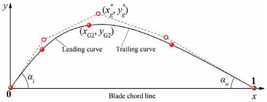
Figure 2.
Blade camberline geometry and parameters.
According to the properties of NURBS curves, when the first and last control points have fourfold knots, the first and last control points of a NURBS curve are the initial and terminal points on the curve itself. Since the leading edge is at (0, 0) and the trailing edge is at (1, 0), then
The derivative at the leading and trailing edge of the NURBS curve equals the slope of the two control points at the leading and trailing edge
then,
Finally, the control point matrix of the blade can be expressed as.
In the actual blade design, we do not know the specific positions of the control points, and we often reverse the control points based on the known interpolation points on the existing blade curves and then construct a NURBS curve with known interpolation points (Figure 2). Assuming that the known blade interpolation point matrix is
The known interpolation point matrix can be substituted into the right side of Equation (16), and the control point matrix can be obtained by matrix calculation. Equation (16) can calculate the control point matrix of the NURBS open curve.
In Equation (16) ai, bi, ci, ei can be expressed as:
di is the control point and pi is the interpolation point. The symbol Δ is introduced to express the length of each knot interval as Δi = ui+1 − ui (i = 0, 1, 2…, n). ui is the knot, subscripted as a sequence of positive constants (i = 0, 1, 2…, n).
Equations (15) and (17) are substituted into Equation (16) to obtain all the unknown control points di, and the calculated control point matrix and Equation (14) are equal to each other to obtain the key geometric parameters of the unit blade camberline. Finally, the NURBS curve of the unit camberline can be obtained by substituting into Equation (1), and the parameterized adjustment of the blade camberline can be realized by adjusting the key geometric parameters.
Unlike the unit blade camberline constructed by a NURBS open curve, the unit blade thickness distribution is constructed by a NURBS closed curve, as shown in Figure 3.
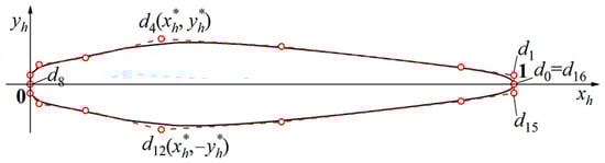
Figure 3.
Thickness distribution model for streamlined torque converter blading.
The thickness distribution curve of the original blade was fitted by 17 interpolation points. The initial interpolation point and the termination interpolation point coincide at (1, 0) and the intermediate interpolation point is at (0, 0). The initial fitting of the thickness distribution profiles will have a sharp angle at the (1, 0) position, which needs to be revised and re-fitted. According to the known interpolation points, 17 control points are inversely calculated (Figure 3). Then, adjust the three control points near (0, 0) to the yh-axis, and adjust the four control points at (1, 0) to the line with xh = 1. At the same time, fourfold knots are used at the (0, 0) and (1, 0) positions so that the curvature of the joint point can be guaranteed to be continuous and the curve can pass through the (0, 0) and (1, 0) positions, which is convenient for the construction of the blade profile in the following.
(b) Parameterization of blade profiles
Before constructing the profiles of the blade pressure side and suction side, the blade camberline posture needs to be adjusted. Mirroring, rotating, and scaling the unit blade camberline (Figure 4), the control point matrix of the 2D profiles of the real unit blade camberline can be obtained.
where γ represents the deflection angle of the blade camberline. For the pump and turbine, it refers to the angle between the blade chord line and the radial baseline, and for the stator, it refers to the angle between the blade chord length and the axial baseline. The counterclockwise rotation is positive and the clockwise rotation is negative. L represents the length of the core and shell curve intercepted by the inlet and outlet edges of the blade on the meridian view.
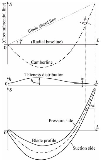
Figure 4.
Blade profile layout.
The real 2D blade profiles can be obtained by overlaying the real thickness distribution on the normal direction of the real blade camberline. The 2D coordinates of the pressure side and suction side of the blade can be calculated by Equation (19).
where subscript p represents the pressure side, s represents the suction side, and c represents the camberline; hi is the blade thickness, ki is the slope of the camberline, is the angle between the camberline normal line and horizontal line; the angle between the normal line and the horizontal line; L denotes the baseline (for pump and turbine refer to the radial baseline, for stator refer to the axial baseline), S denotes the circumferential arc length.
2.3. Parameterized Blade-Fitting Accuracy Evaluation
The comparison between the NURBS and original blades is shown in Figure 5. It can be seen from Figure 5b that the largest errors in the fitting of the pump profiles occur at the leading and trailing edge of the blades. The maximum error is about 0.6 mm at the leading edge of the pressure side, which may be caused by the casting errors of the original blade head, and the average error is within −0.3–0.3 mm. It can be seen in Figure 5a that the maximum error between the pressure side and the suction side of the turbine blade is less than 0.6 mm and the average error is also within −0.3–0.3 mm. Due to the great curvature changes in the turbine blade and the narrow and long turbine blade, the fitting accuracy of the turbine blade has decreased to a certain extent. It can be seen in Figure 5c that the maximum error of the stator blade is below 0.3 mm and the average error is within −0.2–0.2 mm. In summary, the NURBS curve can perform high-precision fitting and parametric expression on the original profiles, which lays a solid foundation for the subsequent optimal design of the cascade system.
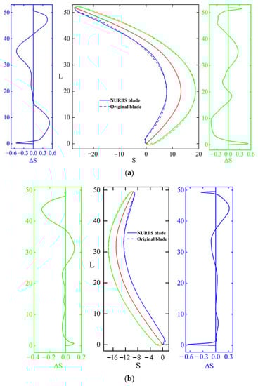
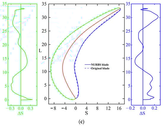
Figure 5.
2D blade profile construction results of hydrodynamic torque converter (a) turbine blade, (b) pump blade, (c) stator blade (the green line on both sides is the fitting error distribution of suction side, the blue line is the fitting error distribution of pressure side, and the middle part is the comparison of cascade modeling results).
2.4. Numerical Method Validation
In this paper, a multi-objective optimization study is carried out on an essential cascade parameter (camberline peak height). The detailed parameters of the camberline peak height of each impeller blade are listed in Table 1. The torque converter’s torus diameter is 380 mm. The CFD model and grid independence study of the hydrodynamic torque converter are shown in Figure 6.

Table 1.
The unit camberline peak height of the original model.
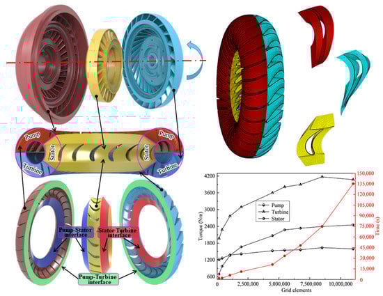
Figure 6.
CFD model of the hydrodynamic torque converter and grid independence study.
In this paper, tetrahedral grids are used to calculate the response surface model (RSM) and multi-objective optimization (fully automated CFD). Finally, hexahedral grids with high precision are used to analyze the flow-field mechanism and capture the secondary flow phenomenon (manual CFD). The global grid element size is 2.4 and the grid elements reach 8.51 × 10⁶ (tetrahedral grids). As shown in Figure 6, increasing the grid size has little effect on the impeller torque but it will significantly increase the computational costs. In order to capture the flow separation phenomenon around the blade (hexahedral grids), the grid near the wall is refined. In order to ensure that y+ is less than 2, the height of the first layer is 0.025 mm and the grid growth rate is 1.2 for the 12-layer grid near the wall. The solver in this paper is calculated by ANSYS Fluent 2021 commercial software. The detailed parameter settings of the CFD calculation are shown in Table 2.
Table 2.
CFD model parameters.
The torque converter external characteristic bench test in this paper is carried out in the hydrodynamic transmission department of Shaanxi Fast Auto Drive Group Company. The experimental prototype and test rig of the hydrodynamic torque converter are shown in Figure 7. The speed ratios (i) of the driving motor (generator) and the load motor (motor) are adjusted according to the setting conditions of the simulation. The impeller torque at different speed ratios is obtained according to the torque and speed sensors on both sides of the torque converter and then the external characteristics are calculated.
Figure 7.
The prototype and test rig of the torque converter: (a) experimental prototype; (b) test rig.
The external characteristics of the torque converter are composed of the torque ratio (K), the efficiency (η), the nominal torque (Tbg), and the high-efficiency region width (Gη) under different speed ratios. (). MT is the turbine torque (Nm), MP is the pump torque (Nm), ωT is the turbine rotational speed (rpm), and ωP is the pump rotational speed (rpm). ηp is the minimum efficiency allowed by the torque converter for normal operating conditions. For engineering machinery, ηp = 0.75, see page 43 of Reference [23]. Gη is the width of the high-efficiency region, indicating the high-efficiency range of the hydrodynamic torque converter under normal operating conditions. The ratio of the high-speed ratio to the low-speed ratio corresponding to ηp= 0.75 can be used to characterize the economic performance of the hydrodynamic torque converter.
The external characteristics of the original blade and NURBS blade (base model) are compared, as shown in Figure 8. On the whole, the external characteristics of the original cascade and NURBS cascade are almost the same (the original cascade is slightly larger than the NURBS cascade at i = 0–0.2, which may be due to the fitting error). The CFD results can achieve an accurate prediction of the original cascade experimental test results and the average error is within 5%. It can be concluded that the parametric expression and construction of the original cascade by the NURBS curve in this paper are successful.
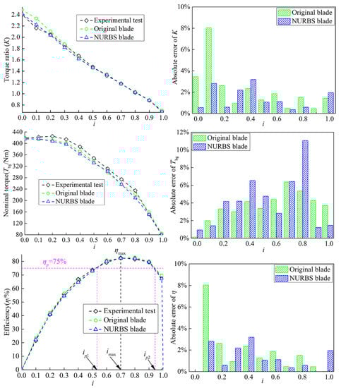
Figure 8.
The comparison of hydrodynamic performances between the simulation and rig test.
3. Optimization Strategy of Hydrodynamic Torque Converter Cascade
3.1. Optimization Problem Description and Constraint Handling
Numerous studies [24,25,26] have shown that the peak height of the blade camberline is very important for the external characteristics of the hydrodynamic torque converter. When the hydrodynamic torque converter is under normal operating conditions, most of the time it is operating in the high-efficiency zone, that is, η ≥ 0.75. The peak efficiency and width of the high-efficiency zone are crucial to the hydrodynamic torque converter and these two indicators determine its economic performance. In engineering practice applications, a greater width of the high-efficiency region and a larger peak efficiency are preferred. Therefore, in the study, the peak height of the camberline of the three impeller blades is used as the independent variable, and the peak efficiency and width of the high-efficiency region are used as the optimization objectives to carry out the multi-objective optimization design. The upper and lower limits of the peak height of the three impeller blades are constrained by the author of this paper. The multi-objective optimization problem of the hydrodynamic torque converter cascade system in this paper can be described by Equation (20).
The optimal Latin hypercube method is often employed to select the sample points because of its uniformity of random sample points [27,28,29]. Therefore, this study selects the optimal Latin hypercube to select the sample space point of the peak height of the blade camberline. In this paper, 30 groups of sample points are evenly selected, and the parametric modeling of the selected 30 groups of sample points is carried out. Then the external characteristics are calculated, and the response surface model (RSM) of the peak height of the blade camberline is established.
3.2. Establishment of Integrated Optimization Platform for 3D Cascade System of Torque Converter
In order to shorten the design cycle and computational costs, the hydrodynamic torque converter cascade system integration optimization platform in the Isight multidisciplinary optimization software is established by the authors. Each process of the cascade design, including the cascade parametric modeling, meshing, flow-field analysis, and optimization design, is integrated by batch and script files (Figure 9). A 3D cascade optimization integrated design platform for torque converters with the CFD as the core and the optimization method as the top-level drive is established, as shown in Figure 9. The three-dimensional cascade system integration optimization platform of the torque converter is as follows: the sample point matrix of the cascade parameters is generated by DOE; the blade profile curve is calculated by Matlab software; the generated blade curve is imported into the UG software, and the parametric modeling and automatic program operation of the full-flow passage of the torque converter are realized by batch and script files; the generated full-flow passage model is imported into the ICEM-CFD software through batch and script files to realize the automatic meshing and output grid model; the generated mesh model is imported into the Fluent software through batch and script files to realize the automatic CFD calculation; a PC with an Intel Xeon Silver 4210R 2.4 GHz CPU and 128 GB of memory was employed for the calculations (20 cores and 40 threads). In this paper, parallel computing is carried out (each Fluent component is assigned 5 cores and 10 threads, a batch of parallel computing consists of four Fluent components: Fluent 0: i = 0, 0.4; Fluent 1: i = 0.5, 0.6; Fluent 2: i = 0.7, 0.8; Fluent 3: i = 0.9, 1.0). Finally, the torque of the impeller is output, the external characteristics of all sample points are calculated, and the response surface model of the cascade parameters is established. Then, the multi-objective optimization of the NURBS cascade can be completed.
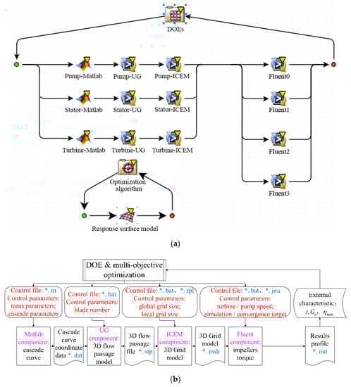
Figure 9.
Integrated optimization system model of 3D cascade system for hydrodynamic torque converter (a) integrated optimization system (Fluent 0: i = 0, 0.4; Fluent 1: i = 0.5, 0.6; Fluent 2: i = 0.7, 0.8; Fluent 3: i = 0.9, 1.0); (b) flow-process diagram.
The peak height of the blade camberline of the hydrodynamic torque converter is optimized by two stages, the automatic CFD stage and the manual CFD stage, as seen in Table 3 in Section 3.2. The optimization process includes two stages: (1) The automatic CFD stage: in order to speed up the calculation and reduce human error, the full-flow passage tetrahedral grid of the hydrodynamic torque converter is automatically divided and the advanced GEKO turbulence model is used for the numerical simulation and multi-objective optimization calculation; (2) The manual CFD stage: the full-flow passage of the hydrodynamic torque converter is manually divided into hexahedral grids and LES is used for the numerical model to capture the separation flow and secondary flow in the internal flow field, and then the flow-field mechanism is analyzed.
Table 3.
Parameter settings of four optimization algorithms.
3.3. Response Surface Model and Multi-Objective Optimization
(a) Response surface model
The cubic response surface model, which includes the main effect, the quadratic effect, the cubic effect, and the third-order or lower-order interaction effect, is employed for the regression analysis
The response surface between the peak height of the camberline and the external characteristics constructed by the third-order regression model is shown in Figure 10. It can be seen in Figure 10 that there is a highly nonlinear relationship between the peak height of the blade camberline and the external characteristics.
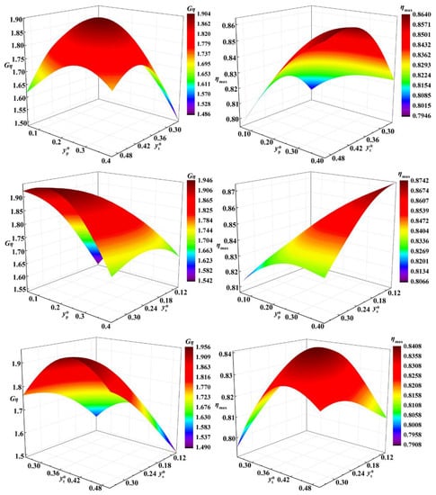
Figure 10.
Nonlinear relationship between parameters and performances.
Ten sample monitoring points are selected to evaluate the fitting accuracy of the response surface model (Figure 11). According to the predicted value of the response surface and the actual calculated values of the 10 sample monitoring points, the R2 value can be calculated by Equation (22). The closer R2 is to 1, the higher the fitting accuracy of the response surface model. It is concluded that the R2 values of Gη and ηmax are 0.99136 and 0.96857, respectively, which are both greater than 0.9, indicating that the response surface model is very reasonable.
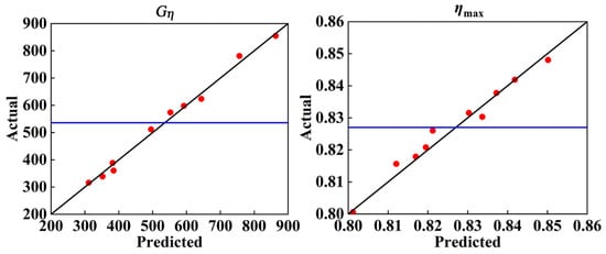
Figure 11.
Precision measurement distribution of sample points. (R2: Gη = 0.99136; ηmax = 0.96857).
The Pareto charts of the nine most significant terms for the two responses are illustrated in Figure 12. For Gη, the quadratic effects of and , the main effect of , and the interaction between and and accounted for −22.32%, −16.91%, 14.44%, −13.04%, and 11.46%, respectively, accounting for 78.17% of the overall contribution rate. For ηmax, the main effect of , the quadratic effect of , and the first-order interaction between , and accounted for 19.29%, −18.36% and 34.08%, respectively, accounting for 71.73% of the overall contribution rate. Overall, in all effects, the factor is crucial to the external characteristics. There is a significant quadratic effect relationship between and ηmax, and there is a significant quadratic effect relationship between and and Gη, which can be clearly seen in Figure 10.
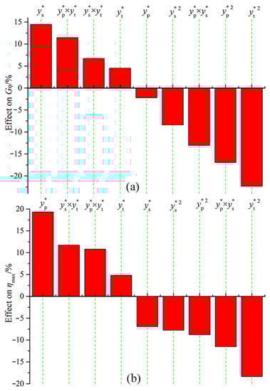
Figure 12.
Pareto charts showing the first 9 primary effects for (a) Gη, and (b) ηmax in the torque converter cascade parameters study.
(b) Multi-objective optimization
Methling et al. [30] used an artificial neural network to predict the stall behavior and state of the four-stage transonic compressor and the results showed that the artificial neural network model could achieve an effective state prediction of the transonic compressor after sufficient training. Poles et al. [31] studied and compared the optimization results of the NSGA-II and MOGA-II optimization algorithms and the results show that there is essentially no difference between the two optimization algorithms. In addition, they also proposed that the reasonable distribution of the initial population can significantly accelerate the convergence of the calculation results. Mariotti et al. [32,33] optimized the diffuser’s contoured cavities using Bezier curves to maximize the pressure recovery and minimize the flow separation, thereby achieving key hydrodynamic performance indicators such as improving diffuser efficiency. In order to avoid the prediction error of the calculation results caused by the different optimization algorithms, the author selects four commonly used optimization algorithms to solve the surrogate model in this paper. The four optimization algorithms are as follows: (1) the archive-based micro genetic algorithm (AMGA); (2) the neighborhood cultivation genetic algorithm (NCGA); (3) the second-generation non-dominated sorting genetic algorithm (NSGA-II); and (4) the multi-objective particle swarm optimization (MOPSO). The detailed parameter settings of the four optimization algorithms are shown in Table 3, and the differences between the four calculation results are also compared in the following sections. Of course, the optimization algorithm is not the only method and the designer can choose the appropriate optimization algorithm according to the actual engineering problems. The NSGA-II optimization algorithm adopted by the author in the previous research [34] in the optimization of the cascade system of the hydrodynamic torque converter can realize the multi-objective optimization of the cascade parameters, so the final adoption is that of the NSGA-II optimization algorithm in this paper.
The whole optimization process adopted in the study is shown in Figure 13.
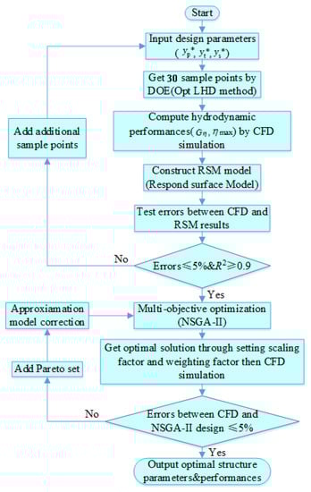
Figure 13.
Multi-objective optimization process.
3.4. Optimization Results
It is important to obtain the Pareto front solution sets with good convexity for the torque converter cascade. In this paper, four optimization algorithms are used to optimize the cascade system of the hydrodynamic torque converter, and the Pareto front solution sets under different optimization algorithms are obtained as shown in Figure 14. It can be seen in Figure 14 that the Pareto front solution sets of these four optimization algorithms are basically the same. The diversity of the Pareto front solutions of the NSGA-II algorithm is the most abundant and the convexity of the solution set is the best. Therefore, this paper finally uses NSGA-II to optimize the solution. Table 4 shows the peak efficiency and high-efficient region width of the optimal torque converter obtained by the different optimization algorithms, and the results of the four algorithms are basically the same. After solving by NSGA-II optimization algorithm, the cascade parameters’ combination of the optimal peak height of the blade camberline can be obtained, as shown in Table 5. Table 6 shows the comparison of the RSM prediction and CFD calculation results of the optimized cascade. The error of the RSM prediction is less than 2%, which demonstrates that the accuracy of the response surface model is very accurate. After optimization, increases from 0.159 to 0.279, increases from 0.369 to 0.371, increases from 0.233 to 0.333, Gη increases from 1.790 to 1.919, and ηmax increases from 0.823 to 0.845 (Table 7). Combined with the response surface analysis in Figure 10, it can be seen that of the optimized cascade is at the maximum value of the quadratic effect relationship, and remains basically unchanged and is near the maximum value of the quadratic effect. has a contradictory relationship with Gη and ηmax, which increases Gη and sacrifices part of ηmax. Overall, the optimized result is a comprehensive optimization scheme, which is consistent with the optimization search direction.
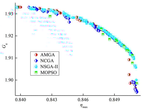
Figure 14.
Comparison of Pareto front solution sets of different optimization algorithms.
Table 4.
Comparison of two objective optimization results of different optimization algorithms.
Table 5.
Comparison of structural parameters before and after optimization.
Table 6.
Comparison of CFD simulation and two-objective optimization results.
Table 7.
Comparison of objectives between the base and optimized models.
4. Results Analysis
4.1. External Characteristics Analysis
The comparison of the external characteristics of the cascade before and after optimization is shown in Figure 15. Compared with the base cascade model, the ηmax and Gη of the optimized cascade increased by 2.673% and 7.207% respectively. Under the normal operating conditions of the torque converter (η ≥ 0.75), the efficiency of the optimized blade is better than that of the base blade. By optimizing the and of the base cascade model, the ηmax and Gη of the torque converter can be significantly improved and at the same time, the other external characteristics indicators are guaranteed to be basically equivalent to the base cascade, which can meet the actual requirements of engineering.
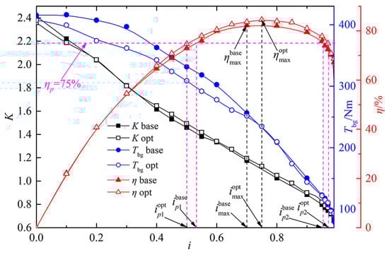
Figure 15.
Comparison of the external characteristics of the cascade before and after optimization.
4.2. Internal Flow-Field Analysis
Figure 16 shows the load distribution on the pump and turbine blades before and after optimization at peak-efficiency operating conditions (i = 0.75). It can be seen from the figure that the pressure distribution on the pump blade before and after optimization is basically the same, demonstrating that the pump torque is basically the same under peak-efficiency operating conditions (it can be seen in Figure 16 that the nominal torque before and after optimization is almost the same under an i = 0.75 operating condition). It can be seen from the efficiency calculation formula that when the pump torque and operating conditions are the same, the efficiency is proportional to the turbine torque. It can be seen in Figure 16b that the turbine torque of the optimized cascade is greater than that of the base cascade, which demonstrates that the peak efficiency of the optimized cascade is greater than that of the base cascade. The dimensionless distance of 0.4 between the suction side of the pump blade and the optimized cascade is the maximum position of the blade curvature, resulting in a decrease in pressure of the suction side. The increase in the pump camberline peak height is crucial to increasing the mass flow rate in the mainstream area of the hydrodynamic torque converter. The increase in the peak height of the pump camberline increases the length of the pump camberline. The larger force area of the pump blade helps to improve the peak efficiency of the hydrodynamic torque converter and reduce the hydrodynamic loss.
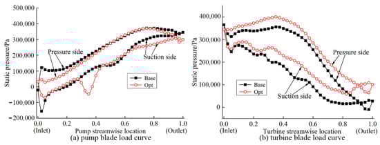
Figure 16.
Comparison of blade load before and after optimization under peak-efficiency operating conditions from inlet (0) to outlet (1).
Figure 17 is the comparison of the velocity field distribution in the pump region before and after optimization. It can be seen in the figure that the increase in the peak height of the pump camberline blade helps to improve the flow rate of the trailing edge of the blade, that is, the mass flow rate of the leading edge of the turbine. Therefore, the hydrodynamic loss is reduced, especially the torque multiplication capacity under peak-efficiency operating conditions is improved, that is, the peak efficiency and the economic performance of the hydrodynamic torque converter are improved.
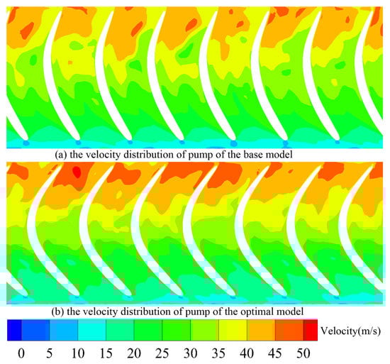
Figure 17.
Comparison of pump flow field before and after optimization under peak-efficiency operating condition.
5. Conclusions
Traditional one-dimensional flow beam theory is discontinuous and cannot realize the accurate adjustment of the blade profile curve. Therefore, in order to make up for defects in the curvature of the hydrodynamic torque converter cascade design, a new parametric design method for a hydrodynamic torque converter cascade based on a NURBS curve is proposed in this paper. In this paper, the parametric modeling, meshing, CFD post-processing, and multi-objective optimization of the hydrodynamic torque converter cascade are integrated, and the integrated optimization design platform of the three-dimensional cascade system of the hydrodynamic torque converter is established. Through the multi-objective optimization of the key parameters of the base model cascade, the economic performance index of the hydrodynamic torque converter can be effectively improved.
The following conclusions can be obtained:
- 1.
- Based on NURBS theory, a new parametric design method for a hydrodynamic torque converter cascade is proposed. In this paper, a cubic NURBS open curve is proposed to construct the parametric structure of the blade camberline, which solves the curvature discontinuity problem in the design of the splicing curve in the traditional blade camberline. A cubic NURBS closed curve is proposed to construct the blade thickness distribution curve, and the problem of sharp angles in the blade thickness distribution is solved by controlling the collinear of the four control points at the trailing edge of the blade thickness, which provides an ideal blade thickness parametric design method for designers. By adjusting the key parameters of the cascade, designers can achieve accurate adjustments of the cascade curve posture.
- 2.
- Four advanced optimization algorithms are used to optimize the key parameters of the parametrically designed NURBS cascade system, and the corresponding external characteristics and internal flow-field characteristics are analyzed:
- (1)
- After optimization, compared with the base model, the peak efficiency ηmax of the optimized cascade is increased by 2.673 %, and the high-efficiency width Gη is increased by 7.207 %, which means that the economic performance of the optimized cascade is greatly improved and the fuel consumption and carbon dioxide emission are reduced.
- (2)
- It can be seen from the comparison of the internal flow-field results of the optimized and the base model cascades that the increase in the peak height of the pump camberline blade helps to improve the flow rate of the trailing edge of the pump blade, that is, the mass flow rate of the leading edge of the turbine. Therefore, the hydrodynamic loss is reduced and the torque multiplication capacity under peak efficiency operating conditions is improved, that is, the peak efficiency and the economic performance of the hydrodynamic torque converter are improved.
- 3.
- The parametric modeling, meshing, CFD post-processing, and multi-objective optimization of the hydrodynamic torque converter cascade are integrated. The integrated optimization design platform for the three-dimensional cascade system of the hydrodynamic torque converter is established, which can greatly reduce artificial errors and shorten the design and optimization cycle of the hydrodynamic torque converter cascade. This will provide great potential and economic value for the development of the hydrodynamic torque converter.
In this paper, the advanced NURBS theory is introduced into the parametric design of the hydrodynamic torque converter cascade system, and a three-dimensional cascade system-integrated optimization design system is built with CFD technology as the bottom design, a control file as the middle layer, and an optimization algorithm as the top drive. The design method of the set of hydrodynamic torque converter cascade systems proposed in this paper provides a new idea for the development of hydrodynamic torque converters. At the same time, the cascade design method and integrated optimization design system can also provide a good reference for engineers for turbomachinery cascade design.
Author Contributions
K.W. and Z.R. performed the data analyses and designed and performed the experiments, and Z.R. wrote the manuscript; B.C. contributed significantly to the analysis and manuscript preparation; K.W. and W.M. contributed to the conception of the study; W.M. and B.C. helped perform the analysis with constructive discussions. All authors have read and agreed to the published version of the manuscript.
Funding
The research is supported by the National Natural Science Foundation of China, grant number 52075212, the Scientific Research Project of the Education Department of Jilin Province, grant number JJKH20220977KJ, the Exploration Foundation of State Key Laboratory of Automotive Simulation and Control, grant number ascl-zytsxm-202010, and the Fundamental Research Funds for the Central Universities, CHD, grant number 300102251511.
Institutional Review Board Statement
Not applicable.
Informed Consent Statement
Not applicable.
Data Availability Statement
The data presented in the study are available on request from the corresponding author.
Conflicts of Interest
The authors declare no conflict of interest.
Nomenclature
| n | Number of control points |
| Weight | |
| di | Control points |
| u | The implicit expression of independent variables |
| NURBS | Non-uniform rational B-spline |
| The basis function of the cubic non-uniform rational B-spline | |
| ui | Knot value |
| U | Knot vector |
| C | NURBS curves |
| k | k-order derivative of NURBS curve |
| pi | Interpolation points |
| Blade inlet angle [degree] | |
| Blade outlet angle [degree] | |
| Blade camberline peak position | |
| Blade camberline peak height | |
| , the length of each knot interval | |
| Blade thickness peak position | |
| Blade thickness peak height | |
| The control point matrix of the 2D profiles of the real unit blade camberline | |
| Deflection angle of the blade camberline [degree] | |
| L | Radial baseline position for pump and turbine/ Axial baseline position for stator |
| S | Circumferential baseline position |
| p | Pressure side |
| s | Suction side |
| Blade thickness | |
| The slope of the camberline | |
| The angle between the camberline normal line and horizontal line [degree] | |
| , speed ratio | |
| K | , torque ratio |
| Turbine torque [Nm] | |
| Pump torque [Nm] | |
| Turbine rational speed [rpm] | |
| Pump rational speed [rpm] | |
| The high-efficiency region width | |
| The minimum efficiency allowed by torque converter for normal operating conditions | |
| K × i, efficiency | |
| The peak efficiency | |
| The nominal torque [Nm] | |
| AMGA | Archive-based micro genetic algorithm |
| NCGA | Neighborhood cultivation genetic algorithm |
| NSGA-II | The second-generation non-dominated sorting genetic algorithm |
| MOPSO | Multi-objective particle swarm optimization |
References
- Schulz, H.; Greim, R.; Volgmann, W. Calculation of three-dimensional viscous flow in hydrodynamic torque converters. ASME J. Turbomach. 1996, 118, 578–589. [Google Scholar] [CrossRef]
- Wollnik, M.; Volgmann, W.; Stoff, H. Importance of the Navier-Stokes forces on the flow in a hydrodynamic torque converter. In Proceedings of the 4th WSEAS International Conference on Fluid Mechanics and Aerodynamics, Elounda, Greece, 21–23 August 2006. [Google Scholar]
- Fuente, P.; Stoff, H.; Volgmann, W.; Wozniak, M. Numerical analysis into the effects of the unsteady flow in an automotive hydrodynamic torque converter. In Proceedings of the World Congress on Engineering 2011, London, UK, 6–8 July 2011. [Google Scholar]
- Wozniak, M.; Pawelski, Z.; Fuente, P.; Ozuna, G. The mutual influence and blade-row interaction between pump and turbine in a hydrodynamic torque converter. Arch. Motoryz. 2012, 1, 83–93. [Google Scholar]
- Xiong, P.; Chen, X.; Sun, H.; Zhong, J.; Wu, L.; Gao, H. Effect of the blade shaped by joukowsky airfoil transformation on the characteristics of the torque converter. Proc. Inst. Mech. Eng. Part D J. Automob. Eng. 2021, 235, 3314–3321. [Google Scholar]
- Xiong, P.; Sun, H.; Zhong, J.; Zhen, C.; Chen, X.; Gao, H. Analysis of the influence of the number of torque converter blades on working performance based on the response surface method. J. Phys. Conf. Ser. 2021, 1748, 022028. [Google Scholar] [CrossRef]
- Zheng, Z.; Liu, Q.; Deng, Y.; Li, B. Multi-objective optimization design for the blade angles of hydraulic torque converter with adjustable pump. Proc. Inst. Mech. Eng., Part C J. Mech. Eng. Sci. 2020, 234, 2523–2536. [Google Scholar] [CrossRef]
- Liu, C.; Yang, K.; Li, J.; Xu, Z.; Wang, T. Performance improvement and flow field investigation in hydraulic torque converter based on a new design of segmented blades. Proc. Inst. Mech. Eng. Part D J. Automob. Eng. 2020, 234, 2162–2175. [Google Scholar] [CrossRef]
- Liu, C.; Yan, Q.; Wei, W. Design and optimization of torque converter stator blade. J. Harbin Inst. Technol. 2016, 48, 114–119. [Google Scholar]
- Hussain, S.; Liu, J.; Sunden, B. Study of effects of axisymmetric endwall contouring on film cooling/heat transfer and secondary losses in a cascade of first stage nozzle guide vane. Appl. Therm. Eng. 2019, 168, 114844. [Google Scholar] [CrossRef]
- Teia, L. New supersonic loss model for the preliminary design of transonic turbine blades and the influence of pitch. ASME J. Turbomach. 2020, 142, 041008. [Google Scholar] [CrossRef]
- Koini, G.; Sarakinos, S.; Nikolos, I. A software tool for parametric design of turbomachinery blades. Adv. Eng. Softw. 2009, 40, 41–51. [Google Scholar] [CrossRef]
- Koini, G.; Sarakinos, S.; Nikolos, I. Parametric Design of Turbomachinery Blades. In Proceedings of the International Conference on Computer as a Tool (EUROCON 2005), Belgrade, Serbia, 21–24 November 2005; Volumes 1–2, pp. 539–542. [Google Scholar]
- Mo, J.; Tan, X.; Qian, J.; Li, T. Application of NURBS in turbine blade parametric design. Therm. Power Gener. 2013, 42, 46–49. [Google Scholar]
- Derksen, R.; Rogalsky, T. Bezier-PARSEC: An optimized aerofoil parameterization for design. Adv. Eng. Softw. 2010, 41, 923–930. [Google Scholar] [CrossRef]
- Rossgatterer, M.; Juttler, B.; Kapl, M.; Della, V. Medial design of blades for hydroelectric turbines and ship propellers. Comput. Graph. 2012, 36, 434–444. [Google Scholar] [CrossRef] [Green Version]
- Braibant, V.; Fleury, C. Shape optimal design using B-splines. Comput. Methods Appl. Mech. Eng. 1984, 44, 247–267. [Google Scholar] [CrossRef]
- Song, K.; Kim, K.; Park, J.; Kook, J.; Oh, J.; Cho, J.; Kim, M. Development of the Integrated Process for Torque Converter Design and Analysis; No. 2008-01-0785; SAE International: Warrendale, PA, USA, 2008. [Google Scholar]
- Shieh, T.; Perng, C.; Chu, D. Torque Converter Analytical Program for Blade Design Process. SAE Trans. 2000, 200, 1646–1652. [Google Scholar]
- Wei, W.; Yan, Q. Study on hydrodynamic torque converter parameter integrated optimization design system based on tri-dimensional flow field theory. SAE Int. J. Fuels Lubr. 2009, 1, 778–783. [Google Scholar] [CrossRef]
- Li, J.; Qing, X.J.; Zhou, S.; Zeng, J. Turbine blade aerodynamic design software: BladeDesign. Gas Turbine Exp. Res. 2011, 24, 11–15. [Google Scholar]
- Ma, W.; Ran, Z.; Liu, C. Quasi-Uniform B-Spline Curve-Based Hydrodynamic Torque Converter Blade Modeling Method: China. 112963515B [P], 10 September 2021. [Google Scholar]
- Ma, W.X. Theory and Design of Hydrodynamic Transmission; Chemical Industry Press: Beijing, China, 2004. [Google Scholar]
- Ke, Z.; Liu, C.; Wei, W.; Yan, Q.; Meng, X. Numerical Simulation of Torque Converter with Different Pump Blade Camber. In Proceedings of the ASME-JSME-KSME 2019 8th Joint Fluids Engineering Conference, San Francisco, CA, USA, 28 July–1 August 2019. [Google Scholar]
- Liu, C.; Xiang, C.; Yan, Q.; Wei, W.; Watson, C.; Wood, H.G. Development and validation of a CFD based optimization procedure for the design of torque converter cascade. Eng. Appl. Comput. Fluid Mech. 2019, 13, 128–141. [Google Scholar] [CrossRef] [Green Version]
- Liu, C.; Wei, W.; Yan, Q.; Morgan, N. Design of Experiments to Investigate Blade Geometric Effects on the Hydrodynamic Performance of Torque Converters. Proc. Inst. Mech. Eng. Part D J. Automob. Eng. 2019, 233, 276–291. [Google Scholar] [CrossRef]
- Liu, C.; Pan, X.; Yan, Q.; Wei, W. Effect of blade number on performance of torque converter and its optimization based on DOE and response surface methodology. Trans. Beijing Inst. Technol. 2012, 7, 689–693. [Google Scholar]
- Liu, C.; Sheng, C.; Yang, H.; Yuan, Z. Design and optimization of bionic janus blade in hydraulic torque converter for drag reduction. J. Bionic Eng. 2018, 15, 160–172. [Google Scholar] [CrossRef]
- Liu, C.; Bu, W.; Xu, D. Multi-objective shape optimization of a plate-fin heat exchanger using CFD and multi-objective genetic algorithm. Int. J. Heat Mass Transfer. 2017, 111, 65–82. [Google Scholar] [CrossRef]
- Methling, F.; Stoff, H.; Grauer, F. The pre-stall behavior of a 4-stage transonic compressor and stall monitoring based on artificial neural networks. Int. J. Rotating Mach. 2004, 10, 10. [Google Scholar] [CrossRef]
- Poles, S.; Fu, Y.; Rigoni, E. The effect of initial population sampling on the convergence of multi-objective genetic algorithms. In Multiobjective Programming and Goal Programming; Barichard, V., Gandibleux, X., T’Kindt, V., Eds.; Springer: Berlin/Heidelberg, Germany, 2009; pp. 123–133. [Google Scholar]
- Mariotti, A.; Buresti, G.; Salvetti, M. Use of multiple local recirculations to increase the efficiency in diffusers. Eur. J. Mech. B Fluids. 2015, 50, 27–37. [Google Scholar] [CrossRef]
- Mariotti, A.; Buresti, G.; Salvetti, M. Control of the turbulent flow in a plane diffuser through optimized contoured cavities. Eur. J. Mech. B. Fluids 2014, 48, 254–265. [Google Scholar] [CrossRef]
- Ran, Z.; Ma, W.; Liu, C.; Li, J. Multi-objective optimization of the cascade parameters of a torque converter based on CFD and a genetic algorithm. Proc. Inst. Mech. Eng. Part D J. Automob. Eng. 2021, 235, 2311–2323. [Google Scholar] [CrossRef]
Publisher’s Note: MDPI stays neutral with regard to jurisdictional claims in published maps and institutional affiliations. |
© 2022 by the authors. Licensee MDPI, Basel, Switzerland. This article is an open access article distributed under the terms and conditions of the Creative Commons Attribution (CC BY) license (https://creativecommons.org/licenses/by/4.0/).