Article

Constrained Image-Based Visual Servoing of Robot Manipulator with Third-Order Sliding-Mode Observer

College of Intelligent System Science and Engineering, Harbin Engineering University, Nantong Street, Harbin 150001, China
*
Author to whom correspondence should be addressed.
Machines 2022, 10(6), 465; https://doi.org/10.3390/machines10060465
Submission received: 21 April 2022 / Revised: 3 June 2022 / Accepted: 9 June 2022 / Published: 11 June 2022
(This article belongs to the Topic Recent Advances in Robotics and Networks)

Abstract

:
A new image-based robot visual servo control strategy based on a third-order sliding-mode observer (TOSM) model predictive control is proposed in this study. This new control strategy solves the problem of robot visual servo control with system constraints and time-varying disturbances when the camera and model of the robot manipulator are uncertain and the joint velocity is unknown. In the proposed method, the joint velocity and system centralized uncertainties are estimated simultaneously based on a third-order sliding-mode observer, and the image-based visual servoing problem is transformed into a nonlinear optimization problem based on a model predictive control method considering both visibility constraints and actuator constraints, which minimizes the predicted trajectory cost function to generate the control signal for each cycle. Simulations were carried out to verify the effectiveness of the proposed control scheme.

1. Introduction

To make robots more intelligent and flexible, they are often equipped with vision sensors as tools for interacting with the outside world. In recent decades, robotic visual servoing has been fully researched and widely used in various areas, such as robotic production logistic [1], robotic service [2,3], robotic navigation and exploration [4,5]. According to the different feedback information from the camera, the visual servoing system can be divided into image-based visual servoing [6,7], position-based visual servoing [8,9], and hybrid visual servoing [10,11]. Refs. [6,7] adopted the image-based visual servoing method, which takes the deviation between the current and desired image features as the control deviation. The robustness of different position-based visual servoing systems was discussed in [8,9], where the control deviations are the deviations of relative pose between the end-effector and the target in the Cartesian coordinate system. The hybrid visual servoing method combines the above two visual servoing methods, and the control deviation is composed of two-dimensional (2D) and three-dimensional (3D) deviations. Refs. [10,11] discussed the applications of the hybrid visual servoing method in mobile robots and parallel robots, respectively. Among these, image-based visual servoing has been the most widely studied and is discussed in this study.
In the image-based visual servo system, the hand-eye mapping relationship is represented by the dynamic relationship between the velocity of the feature points and the joints of the manipulator, which is usually expressed as a Jacobian matrix. Because the Jacobian matrix contains the robot kinematics model and internal and external parameters of the camera, the traditional Jacobian matrix requires a tedious calibration process, and accurate calibration results are difficult to obtain in practical application scenarios. Uncalibrated visual servoing directly defines the error in the image space according to the image features of the manipulator end effector and target and estimates the Jacobian matrix or other nonlinear mapping models during the real-time operation of the system. Yoshimi and Allen proposed an online Jacobian matrix estimation method to solve the jacking task on the plane. In each servo cycle, the manipulator moves through tentative motion and records the image feature changes at the end of the manipulator in the image plane, and uses the parameter identification method. Estimating the current-image Jacobian matrix value, due to its sampling nature, the real-time performance of the system cannot be satisfied [12]. Wang and Liu [13] put forward a neural network algorithm of mixed genetic majorization back-propagation with an aim of model compositing the Jacobian matrix. Zhong put forward an algorithm that combines an Elman neural network and robust Kalman filter to determine the interaction matrix online, taking into account composite noise [14]. The authors of [15,16] both utilize the limit learning machine to evaluate the interaction matrix pseudo inverse for avoiding noise interference and matrix singularity. A six-degree-of-freedom visual servo control method based on image-moments was proposed to solve the problem of underwater vehicle dynamic positioning [17]. In [18], the authors solved the problem of quality inspection of remote radio units (RRUs) through image-based visual servo control. A depth-independent interaction matrix was designed that relates the depth information with the area of the region of interest surrounding the power port in the controller. The stability of the proposed visual servoing controller was analyzed by Lyapunov’s theory. However, the aforementioned studies do not fully consider the linear and nonlinear constraints in visual servoing. For example, if visibility constraints are not considered, the image feature points may be out of the field range of the camera during visual servo control. If the torque constraints are not considered, the joint torque given by the controller may exceed the physical limitation of the robot manipulator. These behaviors will lead to the loss of control quality and failure of the visual servoing task. Therefore, it is crucial to consider the system constraints in designing the controller of visual servoing. One strategy for dealing with constraints is through the path planning technique. In [19], a visual servoing technique based on optimized trajectory planning was proposed to optimize the control process and determine the trajectory parameters by minimizing image-feature deviation. In this technique, the majorization problem is converted into the convex problem, and the trajectory tracking problem for a four-degree-of-freedom manipulator is realized by combining it with the depth-estimation method. The artificial potential field was used in [20] to obtain the initial path, then the initial path was checked and corrected based on the genetic algorithm, and finally, the visual servoing task under the constraint environment was completed. The intelligent control approach has also been utilized to deal with the visual servo system constraint problem. A finite-time optimal control framework was used in [21] to solve feature correspondence and control problems simultaneously, and a small unmanned quadrotor was taken as an example to verify the theoretical research. In [22], a deep reinforcement learning-based visual servo approach was put forward to deal with the problem of feature loss, and an adaptive adjustment controller gain based on DRL was designed to enhance the visual servoing efficiency in the context of meeting the visual field constraints. An approach based on Lyapunov was presented in [23] to realize the semi-global asymptotic (exponential) regulation of the HVS system under unconstrained conditions, and the system’s local asymptotic stability was verified considering the driving-speed constraint. In [24], a method based on the sliding-mode control method was advanced to meet the constraints of robot vision servoing, and 2D and 3D cases were simulated separately. The robustness and feasibility of this approach were confirmed by using the traditional six-axis manipulator. Model predictive control (MPC) methods can solve the constraints explicitly and are often used in constrained systems. Ref. [25] developed a novel visual servo-based model predictive control method to steer a wheeled mobile robot (WMR) moving in a polar coordinate toward the desired target, where kinematic and dynamic constraints are both considered. A predictive controller of visual servo based on the traditional image Jacobian matrix was designed in [26]. A depth-independent Jacobian matrix was used in [27] to verify the robustness of MPC in eye-in-hand (ETH) and eye-to-hand (EIH) visual servoing systems without considering the robot dynamics model. In [28], a quasi-min-max MPC method for visual servoing was presented, in which the depth value is a fixed constant in the Jacobian matrix. In [29], a constrained predictive visual servoing method for fully actuated underwater robots was introduced.
Motivated by the works mentioned above, this paper aims to discuss the visual servoing problem of the robot manipulator considering system model uncertainty, system constraints and time-varying disturbances with the joint velocity unknown using a third-order sliding-mode observer-based model predictive control (MPC-TOSM) method.
The main contributions of this paper are given as follows:
  • A new MPC control strategy is proposed based on the TOSM observer. Considering the nonlinear dynamics of the robot, the MPC controller output the optimal sequence of joint torque with visibility constraints and actuator constraints, and the TOSM observer is employed to observe the system centralized uncertainties together with joint velocities.
  • Compared with the classical traditional control method in [30,31], the proposed strategy in this paper can achieve better servo performance with model errors and system constraints in a 2-DOF robot manipulator. Compared with the recent visual servo control method proposed in [27], the proposed strategy in this paper provides faster convergence speed and more accurate control with time-varying disturbances in both 2-DOF and 6-DOF robot manipulators.
  • The global stability of the system when combining MPC controller and TOSM observer is proved by the Lyapunov stability theory.
These contributions are validated by various comparative experiments.
The residual parts of the paper are organized as follows. Section 2 presents the visual servo model. In Section 3, the sliding-mode observer and MPC controller of the image-based visual servoing are designed. Simulation analysis results are detailed in Section 4. Finally, simulation results that could verify the effectiveness of the proposed image-based visual servo control method are presented in Section 5.

2. Visual Servoing System Modeling

In the current section, the kinematics of visual servoing and robot dynamics modeling are introduced.

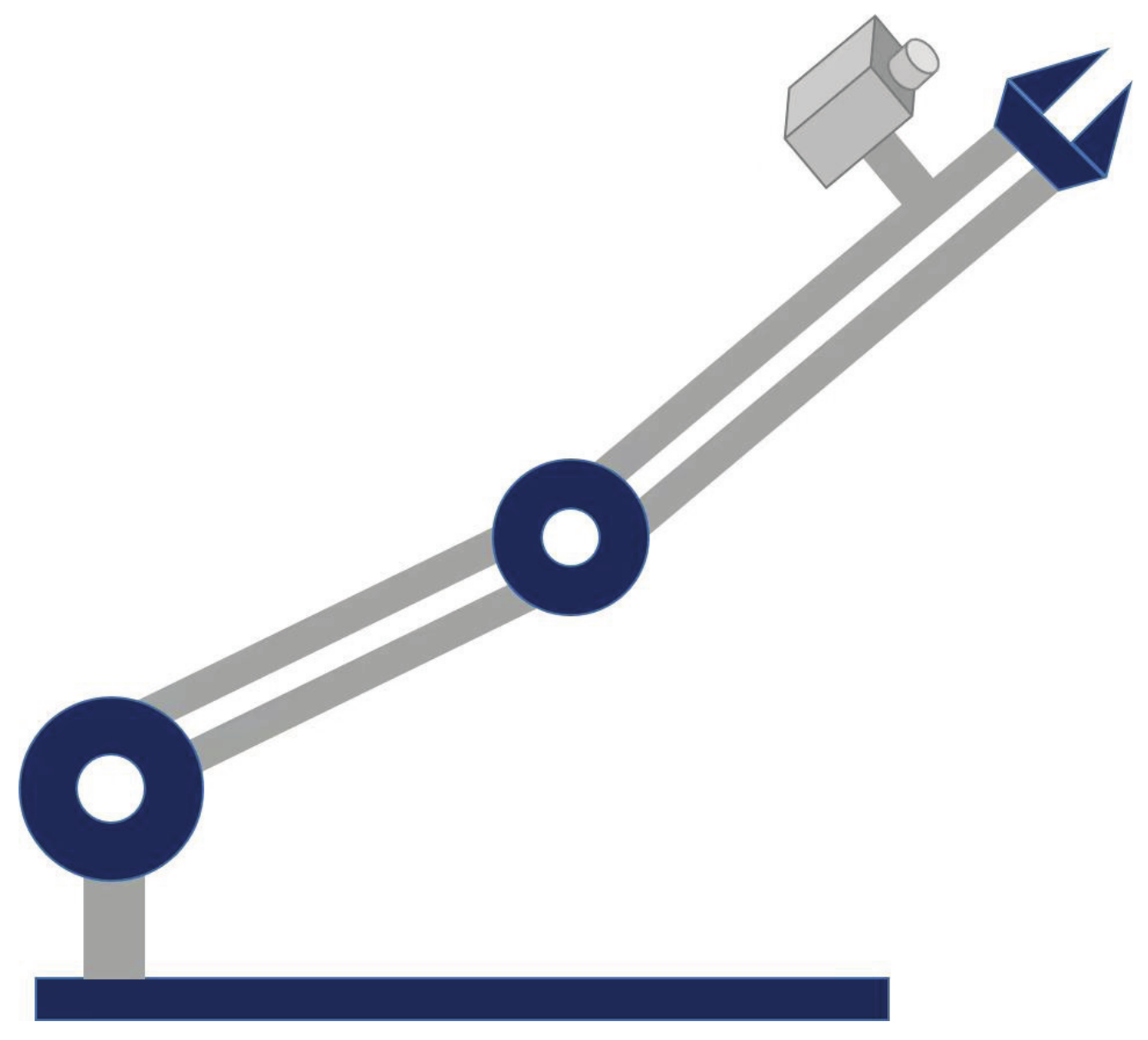
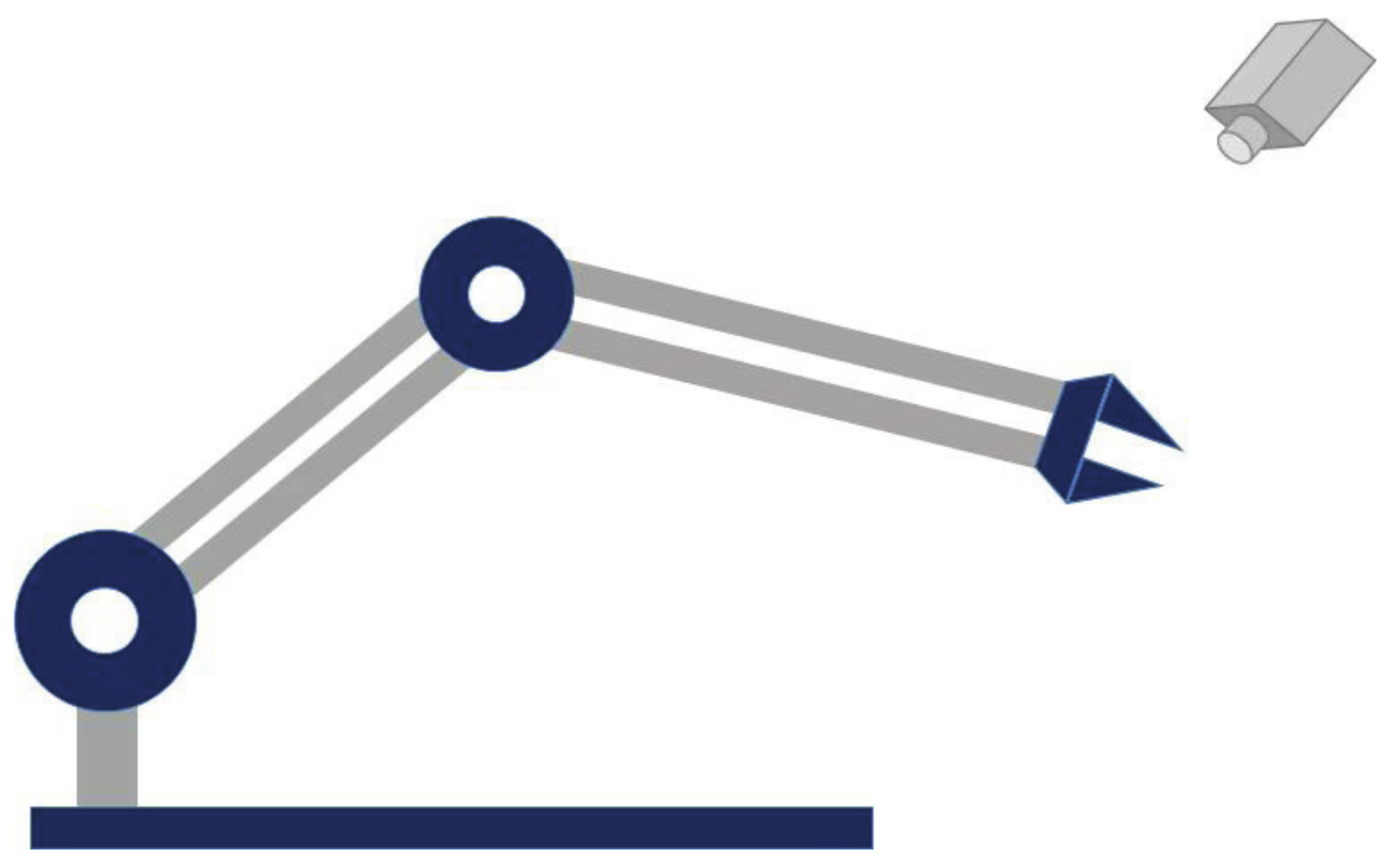
2.1. Kinematics of Visual Servoing Systems

In accordance with the positional correlation between robot and camera, a visual servoing system can be divided to eye-in-hand (EIH) and eye-to-hand (ETH) configurations, as shown in Figure 1 and Figure 2, respectively. In both of these configurations, we give a unified coordinate mapping correlation between the image and camera coordinate system. The feature points in the image coordinate system are defined as s n = ( u n , v n ) T and can be formulated by
s n =   1 z i m 1 T m 2 T Ω y c 1 ,
where z i stands for the depth information of a feature point existing in the camera coordinates, m i T the ith row of the camera parameter matrix which is unknown M 3 × 4 , and Ω 3 × 4 the coordinate transformation matrix which is determined by kinematics, expressed as Ω = R P 0 1 × 3 1 , where R 3 × 3 is a matrix representing the rotation relationship and P 3 × 1 is a matrix representing translation relationship, and y c represents the unknown feature point in Cartesian coordinates.
Different configurations correspond to different matrices. In the configuration of Figure 1, M = D Ω e c , Ω = Ω e b 1 . In the configuration of Figure 2, M = D Ω b c , Ω = Ω e b . The above symbols are defined as follows.
D 3 × 4 is a matrix that involves the camera’s internal parameters, Ω e c stands for the coordinate transformation matrix of the robot base framework relative to the camera framework, Ω e b represents the coordinate transformation matrix of the robot base relative to the end-effector framework relative to the robot base framework, and it can be gathered from the forward kinematics of robot, and Ω b c the coordinate transformation matrix of the robot base framework relative to the camera framework.
The depth z i can be expressed as
z i = m 3 T Ω y c 1 .
Differentiating the above formula relative to time, we can acquire the relationship between the joint velocity and variation of the feature point with time as
s ˙ n = 1 z i C q ˙ ,
where q ˙ R n × 1 denotes the velocity of robot joints, n the freedom degrees of the robot, and C R 2 × n the image Jacobian matrix where the depth is independent, which is expressed as
C = m 1 T u n m 3 T m 2 T v n m 3 T 1 q Ω y c 1 .
The unknown robot kinematic parameters together with the camera parameters identified the components of the depth-independent image Jacobian matrix. In the above formula, both the Jacobian matrix and depth information in it are nonlinear. Therefore, the following properties are introduced herein, and the nonlinear elements are linearized by the regression matrix and unknown parameter vector.
Property 1.
The product D η for a vector η n × 1 can be parameterized linearly as below equations:
D η = B s n ,   η ,   q θ ,
d T η = b s n ,   η θ ,
where B s n ,   η ,   q , b s n ,   η denote the regression matrices, while θ represents the associated unknown parameter vector identified through the products of the unknown robot kinematic parameters together with the unknown camera parameters.
Property 2.
The depth z i can be expressed as the unknown parameters linear form as below
z i = Y q θ z ,
where Y q represents the regression matrix, while θ z stands for the unknown parameters influenced via the products of an unknown camera parameters together with feature position.

2.2. Robot Dynamics

The dynamic control system of robot manipulators can be regarded as a kind of second-order uncertain nonlinear system. The dynamic model of the robot manipulator is given in Lagrangian form as follows:
H q t q ¨ t + K q t ,   q ˙ t q ˙ t + G q t = τ t + τ e t ,
where H q t n × n denotes the inertia matrix, K q t , q ˙ t denote the centripetal and Coriolis torque matrix, G q t n × n the gravitational torques, τ t n × 1 the input torque vector, and τ e t n × 1 the slowly varying external disturbances.
The modeling deviation between the real and mathematical models Δ H 0 q t , Δ K 0 q t ,   q ˙ t , and Δ G 0 q t can be expressed as
Δ H q t = H q t H 0 q t ,
Δ K q t ,   q ˙ t = K q t ,   q ˙ t K 0 q t ,   q ˙ t ,
Δ G q t = G q t G 0 q t ,
respectively, where H 0 q t , K 0 q t ,   q ˙ t , and G 0 q t denote the corresponding nominal parts of the model. Then, Equation (8) can be written as
H 0 ( q ( t ) ) q ¨ ( t ) +   K 0 ( q ( t ) ,   q ˙ ( t ) ) q ˙ ( t ) + G 0 ( q ( t ) ) = τ ( t ) + τ e ( t ) Δ H ( q ( t ) ) q ¨ ( t ) Δ K ( q ( t ) ,   q ˙ ( t ) ) q ˙ ( t ) G ( q ( t ) )
By defining variables F ( q ,   q ˙ ,   t ) ,
F ( q ,   q ˙ ,   t ) = τ e t Δ H q t Δ K q t ,   q ˙ t Δ G q t ,
Equation (12) can be rewritten as
H 0 q t q ¨ t + K 0 q t ,   q ˙ t q ˙ t + G 0 q t = τ t + F ( q ,   q ˙ ,   t ) .
The joint acceleration can be expressed as
q ¨ t = H 0 q t 1 K 0 q t ,   q ˙ t q ˙ t H 0 q t 1 G 0 q t + H 0 q t 1 τ t + H 0 q t 1 F ( q ,   q ˙ ,   t ) .
Considering the uncertain parameters and external disturbances, the approximate dynamic model can be defined as
q ¨ t = f q t ,   q ˙ ( t ) + Δ f ,
where f q t ,   q ˙ ( t ) = H 0 q t 1 K 0 q t ,   q ˙ t q ˙ t H 0 q t 1 G 0 q t + H 0 q t 1 τ t , Δ f = H 0 ( q ( t ) ) 1 F ( q ,   q ˙ ,   t ) .

3. Third-Order Sliding-Mode Observer

As a multi-variable complicated nonlinear system with multi-variable and strong coupling characteristics, the manipulator is easily affected by various internal and external factors during operation, and its own joint velocity measurement is often accompanied by noise. At the same time, it is difficult to ensure the modeling accuracy and hand-eye calibration accuracy of the manipulator in the visual servo system. Therefore, in the current section, a third-order sliding-mode observer is introduced to estimate the system speed and centralized uncertainty, and then the estimated information is input to the model predictive controller as a feed-forward signal. The robot dynamics model (15) is reconstructed into state space equations.
Variables x 1 = q , x 2 = q ˙ are proposed to rewrite the kinetic model as
x ˙ 1 = x 2
x ˙ 2 = f x + g x u t + Π x ,   t
where f x = H 0 q t 1 K 0 q t ,   q ˙ t q ˙ t G 0 q t , g x = H 0 q t 1 ,
u ( t ) = τ ( t ) , and Π x ,   t = H 0 q t 1 F ( q ˙ ,   q ,   t ) .
The following TOSM observer is presented:
x ^ ˙ 1 = σ 1 | x 1 x ^ 1 | 2 / 3 s i g n x 1 x ^ 1 + x ^ 2
x ^ ˙ 2 = f ( x ^ ) + g ( x ^ ) τ ( t ) + σ 2 x 1 x ^ 1 1 / 3 s i g n x 1 x ^ 1 y ^
y ^ ˙ = σ 3 sign x 1 x ^ 1
where x ^ denotes the observation value of the disturbance observer and σ 1 , σ 2 , σ 3 denotes the suitable observer gain value. Subtracting (17) and (18) to (19)–(21), and defining the system state’s estimation errors x ˜ = x x ^ , we have
x ˜ ˙ 1 = σ 1 | x ˜ 1 | 2 / 3 s i g n x ˜ 1 + x ˜ 2
x ˜ ˙ 2 = σ 2 | x ˜ 1 | 1 / 3 s i g n x ˜ 1 + Π ^ x , x ^ , t + y ^
y ^ ˙ = σ 3 s i g n x ˜ 1
By introducing variables y ^ 0 = Π ^ x , x ^ , t + y ^ , the sliding-mode observer becomes
x ˜ ˙ 1 = σ 1 | x ˜ 1 | 2 / 3 s i g n x ˜ 1 + x ˜ 2
x ˜ ˙ 2 = σ 2 | x ˜ 1 | 1 / 3 s i g n x ˜ 1 + y ^ 0
y ^ ˙ 0 = σ 3 s i g n x ˜ 1 + Π ^ ˙ x ,   x ^ ,   t
The estimation errors (25)–(27) is the standard form of the second-order robust accurate differentiator, and its finite-time stability has been successfully proved in [32].

4. MPC Controller Design

In the preceding section, joint velocities and system centralized uncertainty were effectively estimated by designing an SMO. In this section, an MPC-based controller is designed for solving system constraints and model uncertainty, so that image feature points converge to expected values. Figure 3 reflects the overall control scheme. The control instruction is the joint torque of the robot manipulator and the output is the joint angle q. The system uncertainty is estimated using an SMO in the feedforward loop.
The model predictive controller obtains the optimal control input for each control cycle by solving a constrained optimization problem. The design of the model predictive controller is described below.
The visual servo system model is represented by the following discrete-time model:
s n k + 1 q ˙ k + 1 = s n k q ˙ k + 1 z i C k q ˙ k T d ( f q t ,   q ˙ ( t ) + Δ f ) T d ,
where T d denotes the sampling period. The servoing system control inputs can be counted through dealing with the below constrained finite-time optimization problem:
J ( k ) = i = 1 N p s ¯ ( k + i ) s d Q F 2 + i = 1 N p q ˙ ¯ k + i Q G 2 + i = 1 N c τ ¯ k + i 1 R 2
where s ¯ k + i , q ˙ ¯ k + i , and τ ¯ k + i 1 denote the image which is predicted by the MPC, joint velocity, and output torque, respectively, to be modified at time k. s d denotes the desired coordinates of image features. N p denotes the prediction step length, horizon and N c the control step length, which is usually N c N p . The cost function J k consists of three parts: image-feature bias, joint velocity, and torque. Q F 0 , Q G 0 and R represent the associated weighting matrices.
The MPC-based visual servo system with constraints can be described as
Ψ min J k q ˙ k .
To make sure that the feature points are in the camera’s visual field, the visibility constraint is defined as
s n min s n ( k ) s n max ,
where s n min and s n max denote the range of coordinates, respectively, of the image plane.
The torque constraint is expressed as
τ min τ ( k ) τ max ,
where τ min and τ max stand for the boundary value of the force torque. The sequential quadratic programming (SQP) algorithm is an algorithm that converts complex nonlinear constrained optimization problems into simpler quadratic programming (QP) problems. Therefore, this paper adopts the SQP algorithm for the optimal control problem.
The Lyapunov function is defined as as follows:
V k = i = 1 N s ¯ k + i s d Q F 2 + i = 1 N q ˙ ¯ k + i Q G 2 + i = 1 N τ ¯ k + i 1 R 2
Here, for the sake of brevity, the control time domain and the prediction time domain are made equal, that is N P = N C = N . Let
R i = s ¯ k + i s d Q F 2 + q ˙ ¯ k + i Q G 2 + τ ¯ k + i 1 R 2 ,   i I 1 , N
then
V ( k + 1 ) = min τ i = 1 N s ¯ ( k + i + 1 ) s d Q F 2 + i = 1 N q ˙ ¯ ( k + i + 1 ) Q G 2 + i = 1 N τ ¯ ( k + i ) R 2 = min τ i = 1 N R ( i ) R ( 1 ) + R ( N ) = R ( 1 ) + min τ i = 1 N R ( i ) + R ( N ) R ( 1 ) + V ( k ) + min τ i = 1 N R ( N )
and R ( 1 ) 0 , min τ i = 1 N R ( N ) = 0 . As a result, V ( k + 1 ) V ( k ) , namely, V ( k + 1 ) V ( k ) 0 .
Therefore, the stability of the closed-loop system is proven.

5. Simulation Results

In order to verify the effectiveness and robustness of the MPC-TOSM method, the comparative simulations are carried out in this section.

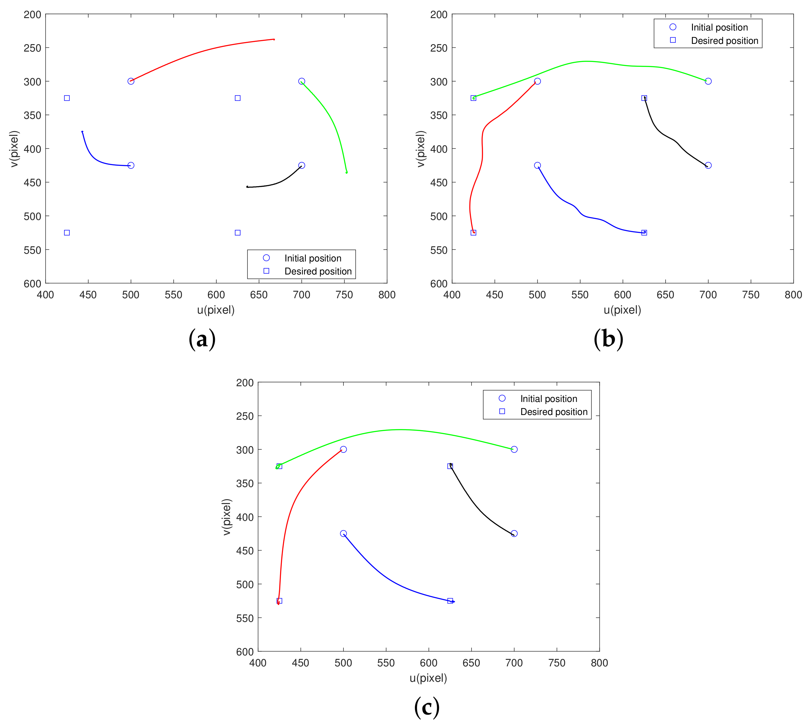
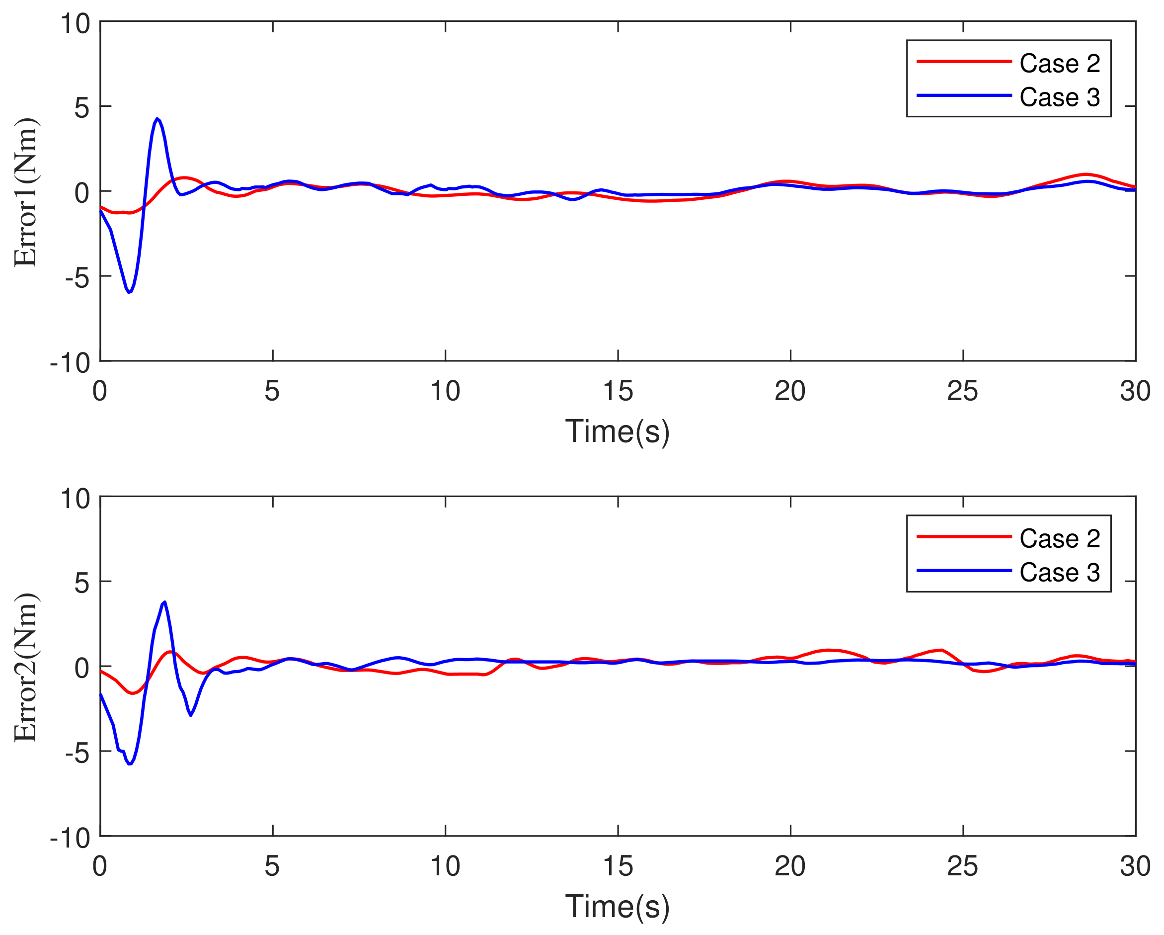
5.1. Comparative Simulations with Model Uncertainty

First of all, the comparative simulations of visual servoing with model uncertainty are carried out in this part. Three control strategies used for the comparative simulations are shown below.
  • Case 1: The control strategy is the traditional visual servo control method in [30].
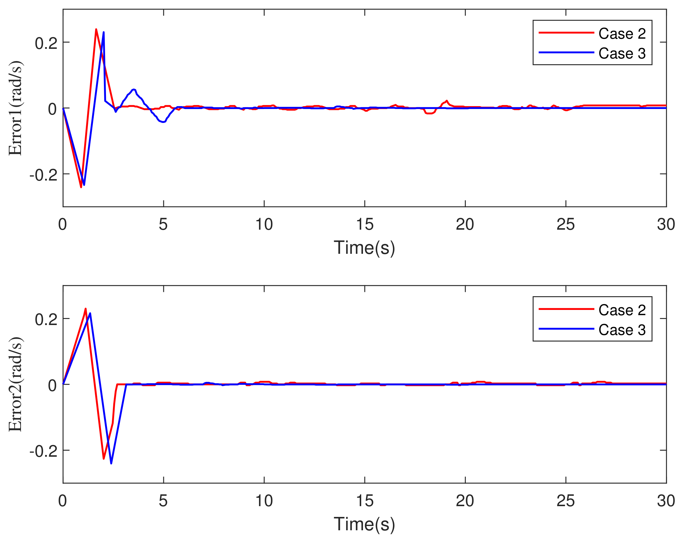
  • Case 2: The control method is MPC and the observer is a traditional SMO in [31].
  • Case 3: The control strategy is the MPC-TOSM method proposed in this paper.
The simulation object adopts the two-degree-of-freedom (2-DOF) manipulator from [27]. In the parameters of the 2-DOF robot manipulator, for the first and second links, their lengths, masses, mass centers and inertia are expressed as l 1 and l 2 , m 1 and m 2 , l c 1 and l c 2 , I 1 and I 2 , respectively. In the initial rough parameters of the 2-DOF robot manipulator, for the first and second links, their lengths, masses, mass centers and inertia are expressed as l ^ 1 and l ^ 2 , m ^ 1 and m ^ 2 and l c 2 , l ^ c 1 and l ^ c 2 , I ^ 1 and I ^ 2 , respectively. The specific values are shown in Table 1 and Table 2.
Furthermore, we assume that the exact camera parameters are unknown in the comparative simulations. The real camera parameters and initial rough camera parameters are shown in Table 3. In this paper, the focal length is denoted by f.The real and initial rough coordinates of the camera stagnation point are u 0 ,   v 0 and u ^ 0 ,   v ^ 0 , which are in the image frame. The real and initial rough scaling factors along the u and v axes are k u ,   k v and ( k ^ u ,   k ^ v ) . The range of the u axis are u min = 0 , u max = 1292 pixels. The range of the v axis are v min = 0 , v max = 964 pixels. The minimum and maximum torques of the actuator are −t10 Nm and 10 Nm. Both visibility constraints and actuator constraints manifest in the visual servoing task. The real and initial rough camera parameters are shown in Table 3.
The Cartesian coordinates of Feture Point 1 to Feture Point 4 that relative to the robot base are 0.0618 , 0.0516 , 0.3 T m, 0.0159 , 0.0516 , 0.3 T m, 0.0618 , 0.023 , 0.3 T m, and 0.0159 , 0.023 , 0.3 T m, respectively. The initial 2D coordinates of the image feature points are 500 , 300 T pixels, 700 , 300 T pixels, 500 , 425 T pixels, and 700 , 425 T pixels. The desired 2D coordinates of the image-feature points are 425 , 525 T pixels, 425 , 325 T pixels, 625 , 525 T pixels, and 625 , 325 T pixels. The initial states of robot manipulator are chosen as q 1 ( 0 ) = q 2 ( 0 ) = π 6 , q ˙ 1 ( 0 ) = q ˙ 2 ( 0 ) = 0 . The coordinate transformation matrix of the end-effector framework relative to the camera framework H c e is expressed as
H c e = 1 0 0 0.01 0 1 0 0.02 0 0 1 0.015 0 0 0 1 .
In the experiments, setting the initial rough estimation of camera extrinsic parameter matrix H ^ c e as
H ^ c e = 1 0 0.25 0.005 0 1 0 0 0 0 0.95 0.01 0 0 0 1 .
The parameters in the third-order sliding mode are chosen as σ 1 = 2.2 L 1 / 3 , σ 2 = 2 L 2 / 3 , σ 3 = L , with L = 6 . The parameters in the MPC controller are chosen as Q F = 30 I 8 × 8 , Q G = 0 I 2 × 2 , and R = 5 I 2 × 2 , N p = 10 , and N c = 8 .
With an aim of comparing the control effects of several methods, the same initial positions of the image features are set, which are represented by circles in Figure 4, and the same desired positions of the image features are represented by boxes. Figure 4 displays the trajectories of features in the image plane in Case 1, 2, and 3 control strategies, respectively. The trajectories of Feture Point 1 to Feture Point 4 are shown in red, green, blue and black, respectively. In Case 1, the rough initial parameters make the classical image-based visual servoing invalid, the feature points deviate from the desired positions, and the visual servoing task cannot be completed. In Case 2 and 3, the image features both reach the desired final position. However, the trajectory of image features fluctuates during the convergence process in Case 2. In Case 3, the trajectory of image features converges to the desired position smoothly and quickly. Figure 4c indicates that the proposed method can obtain satisfactory control effects without joint-angle measurement in the company of visibility constraints, actuator constraints, and system model uncertainty. Figure 5 displays the feature response deviations in the image plane in Case 1, 2, and 3 control strategies, respectively. The deviation is defined as the difference between the current feature point coordinates and the desired point coordinates. In Figure 5b,c, it can be seen that the stabilization time of the control system is about 10 s in Case 3, faster than in Case 2 (15 s). In Figure 6, it can be observed that the traditional SMO control strategy leads to the chattering phenomenon of the joint torques, while the proposed MPC-TOSM method can suppress the chattering phenomenon effectively and better complete the visual servo goals. Figure 7 and Figure 8 display the estimation errors of the joint velocities together and the uncertainty estimation errors of the observers in Case 2 and Case 3. We can see that the TOSM observer has higher estimation accuracy than the traditional sliding mode observer. Higher estimation accuracy brings better control performance to the control system.

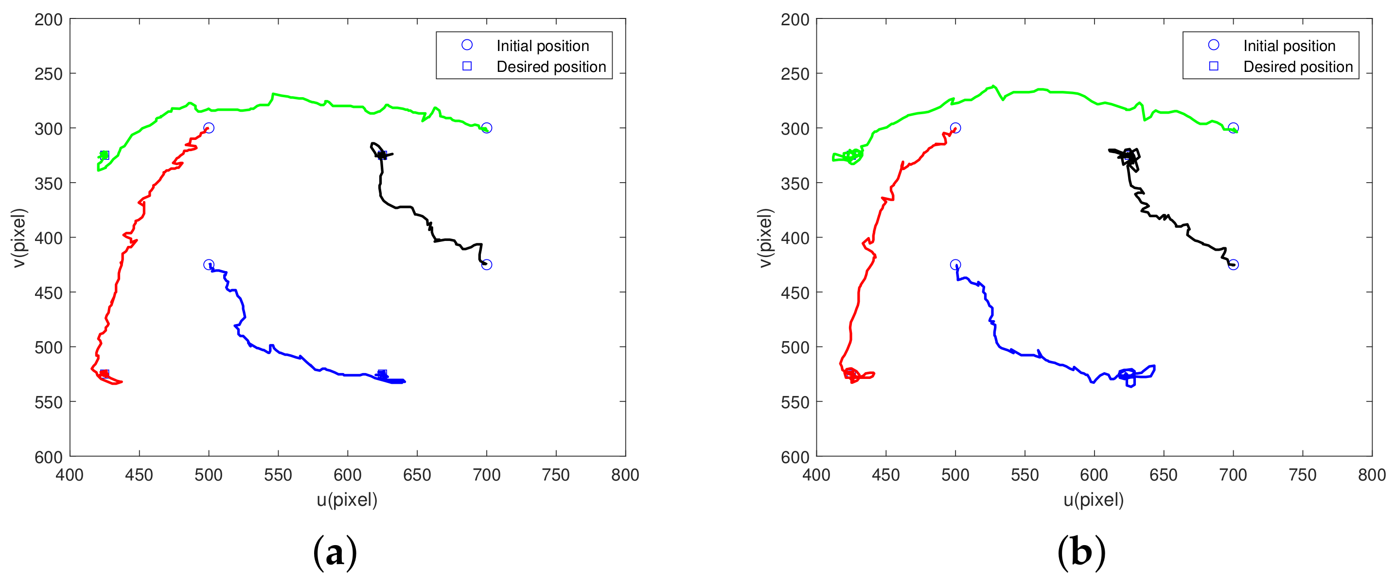
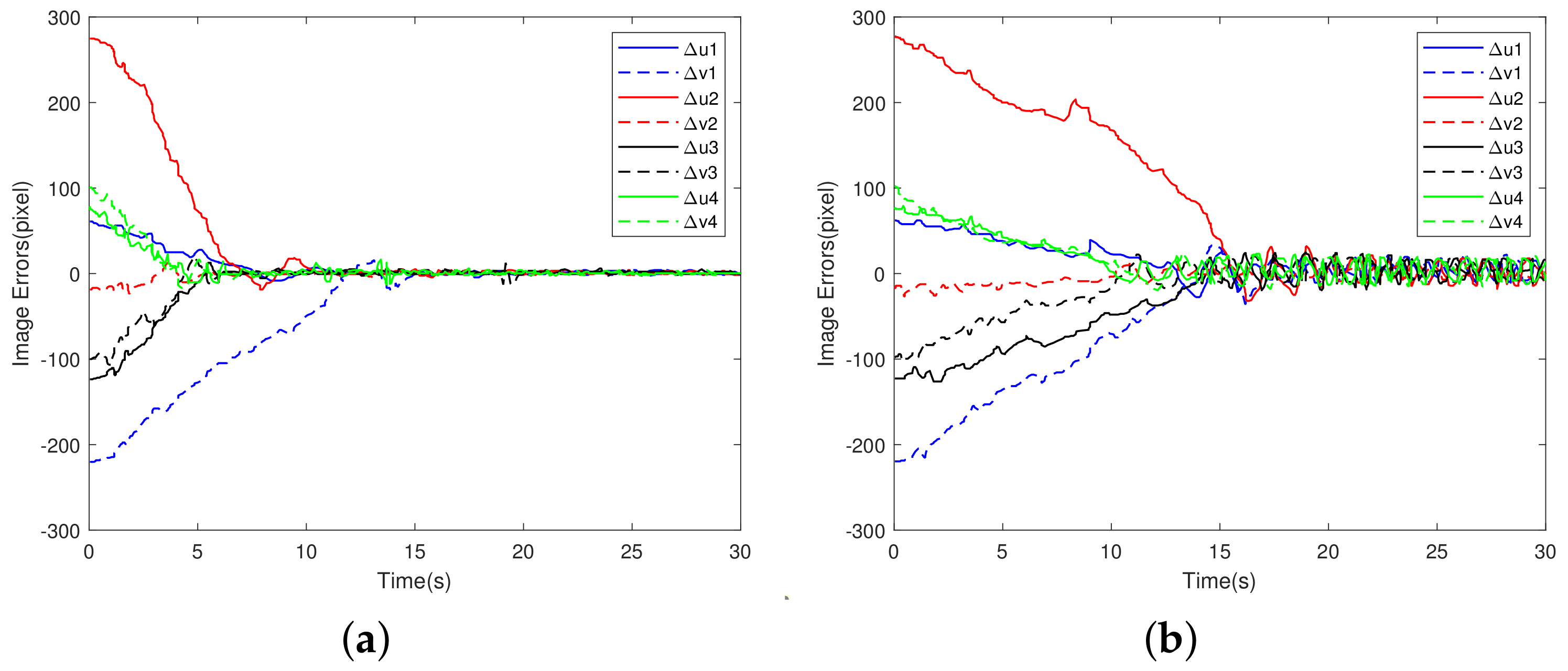
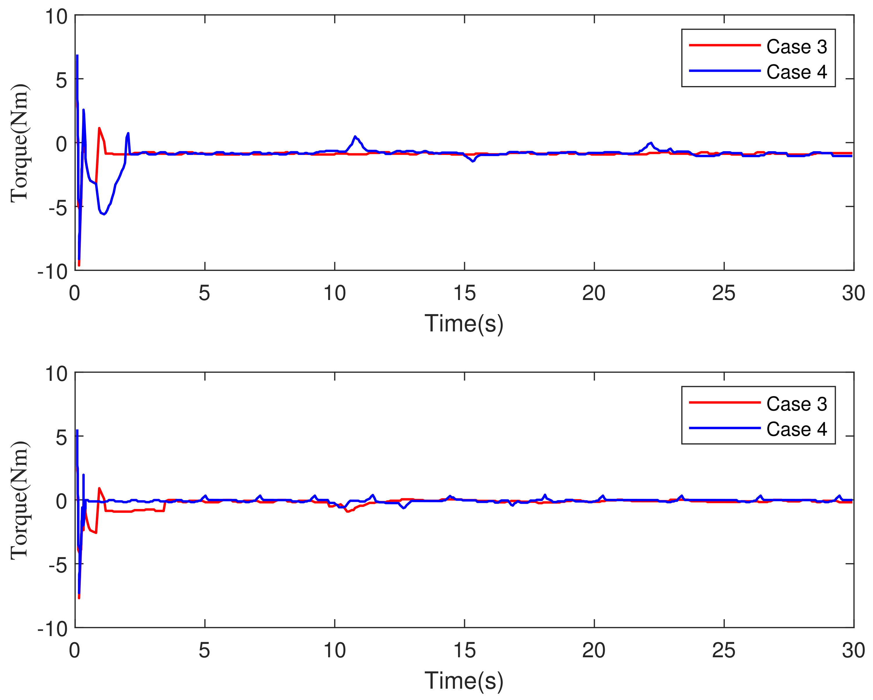
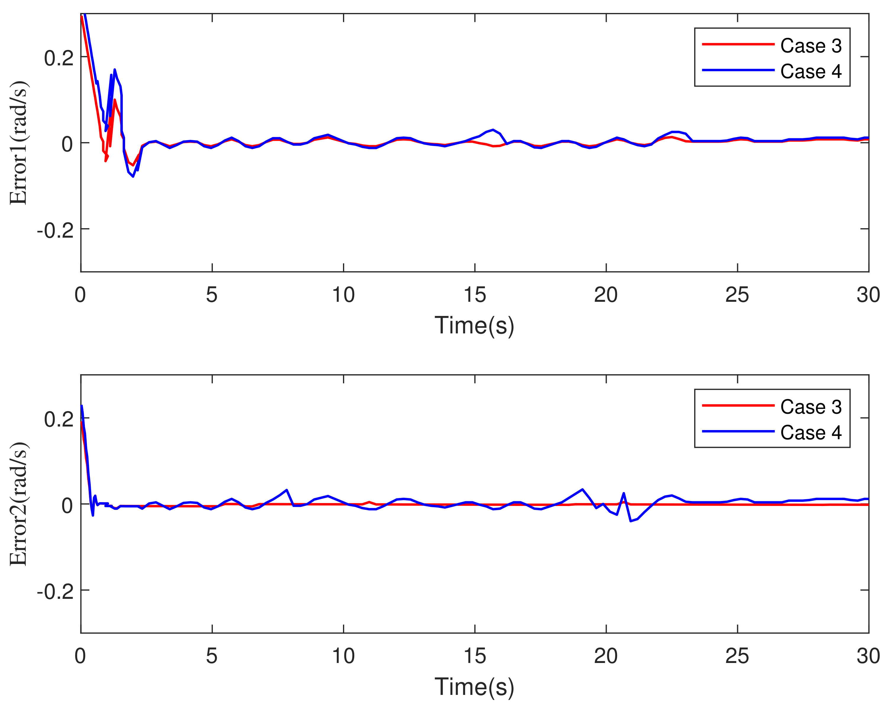
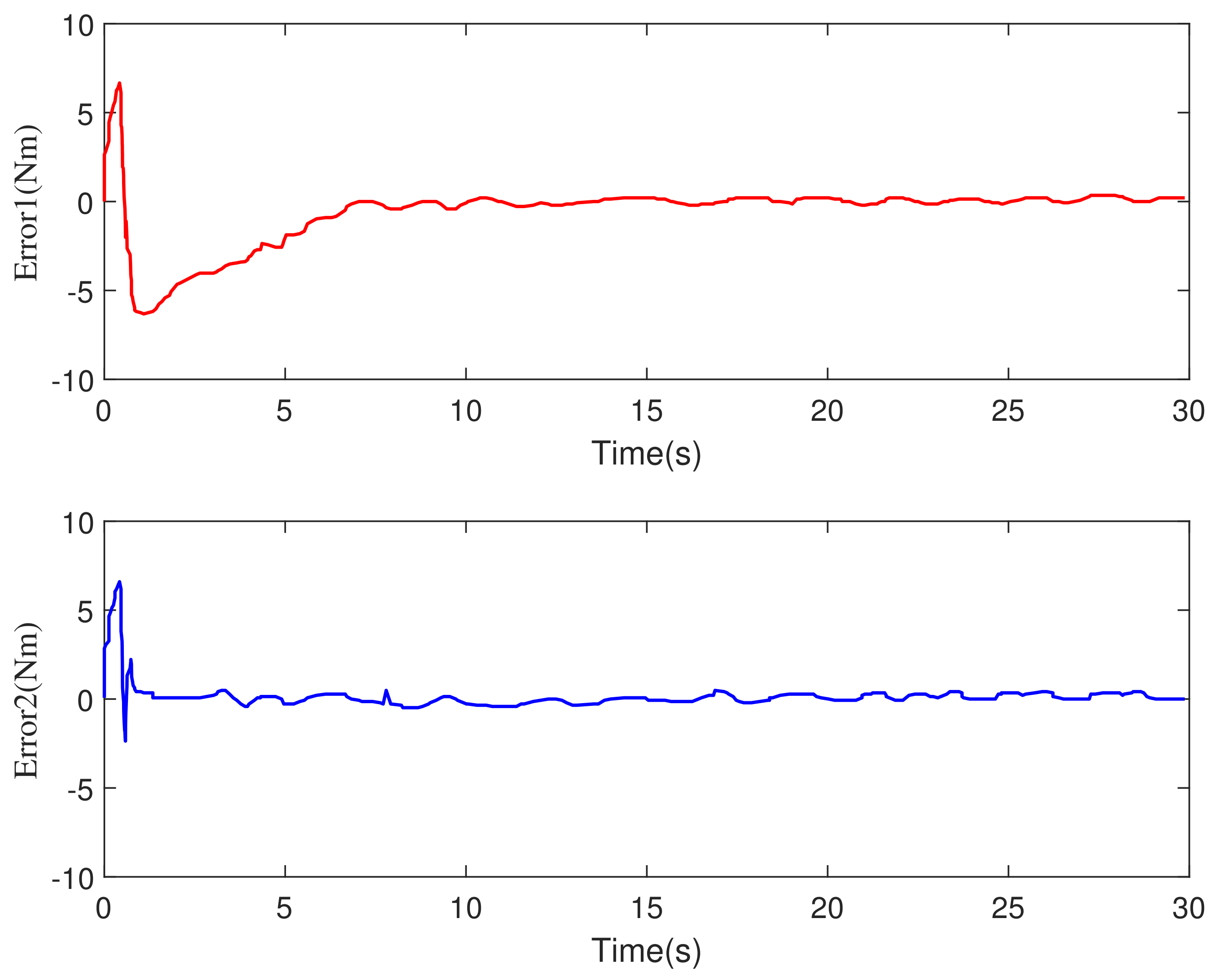
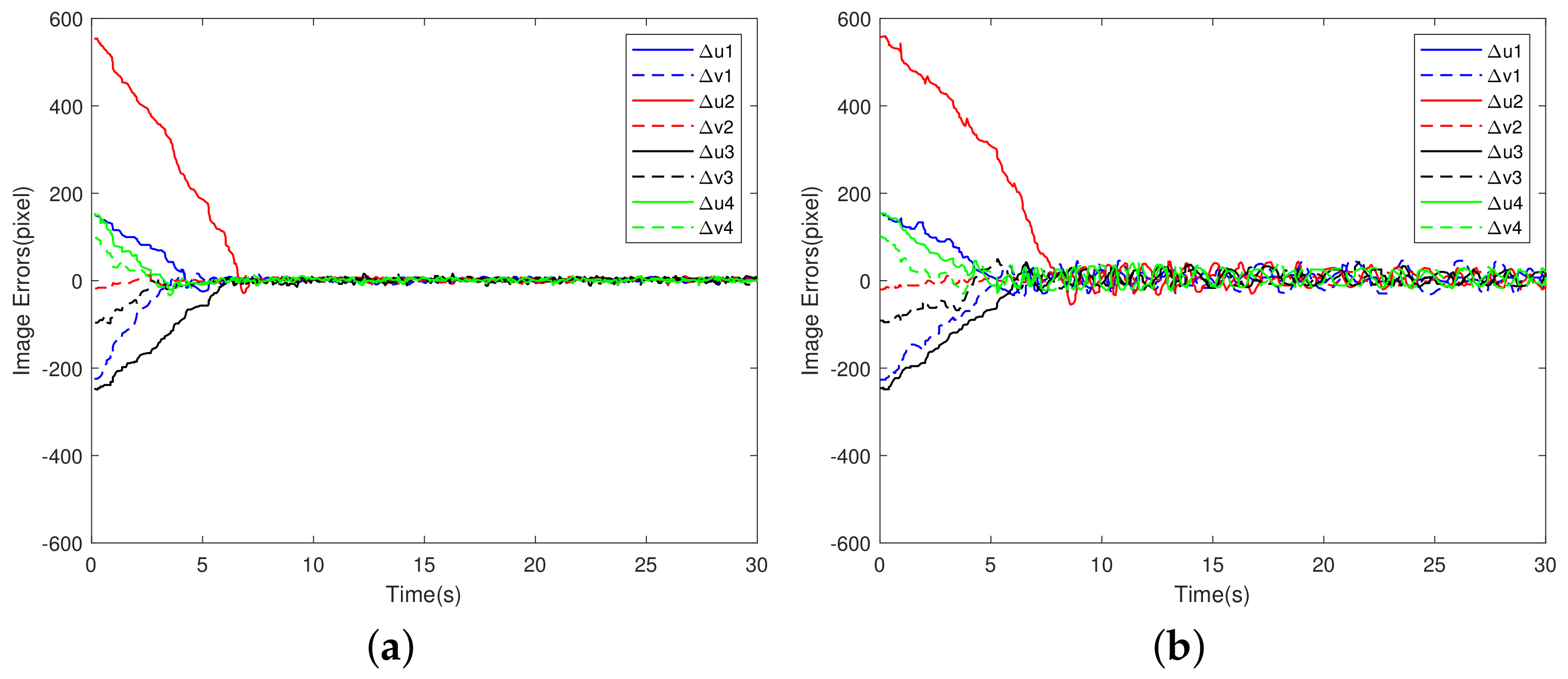
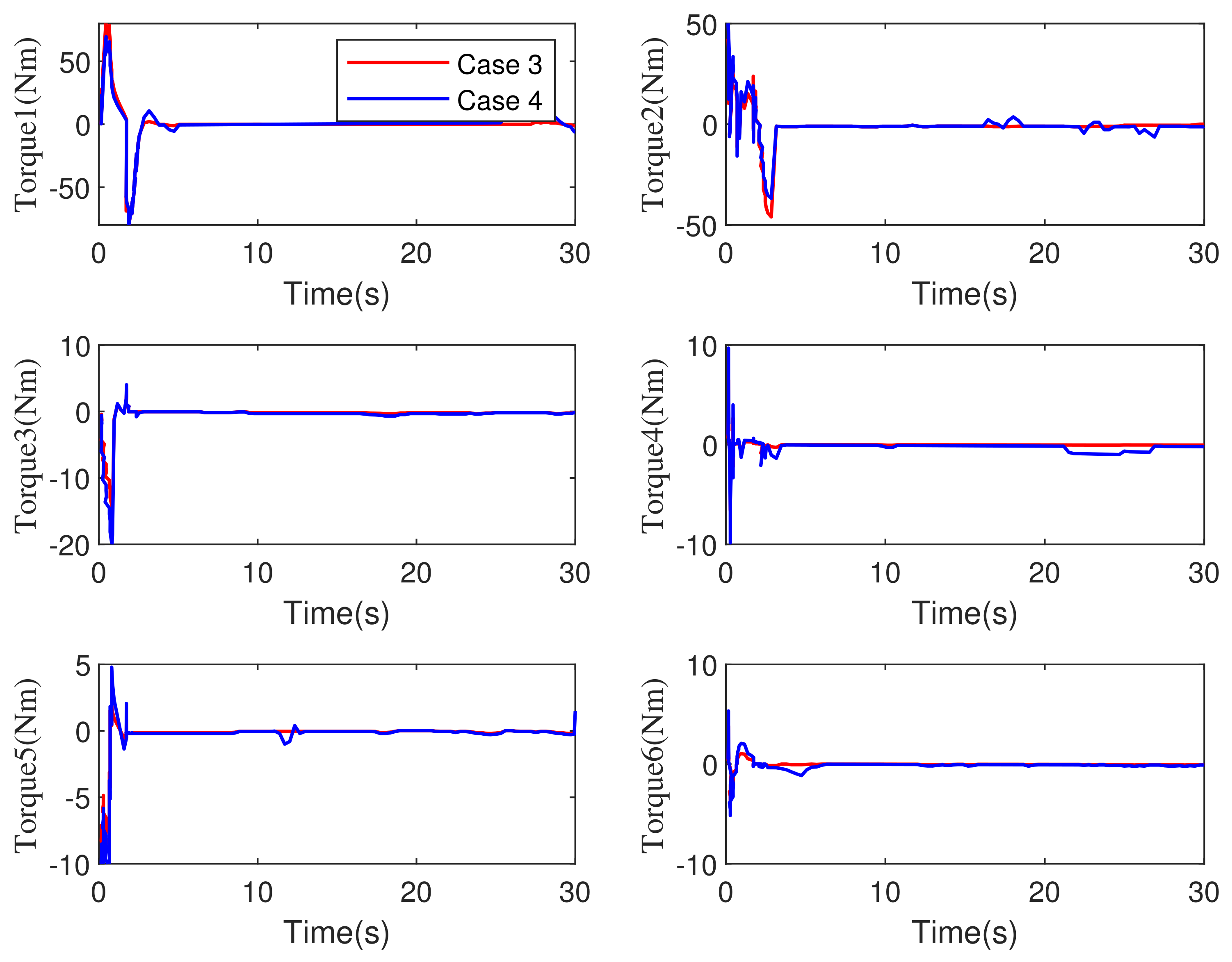
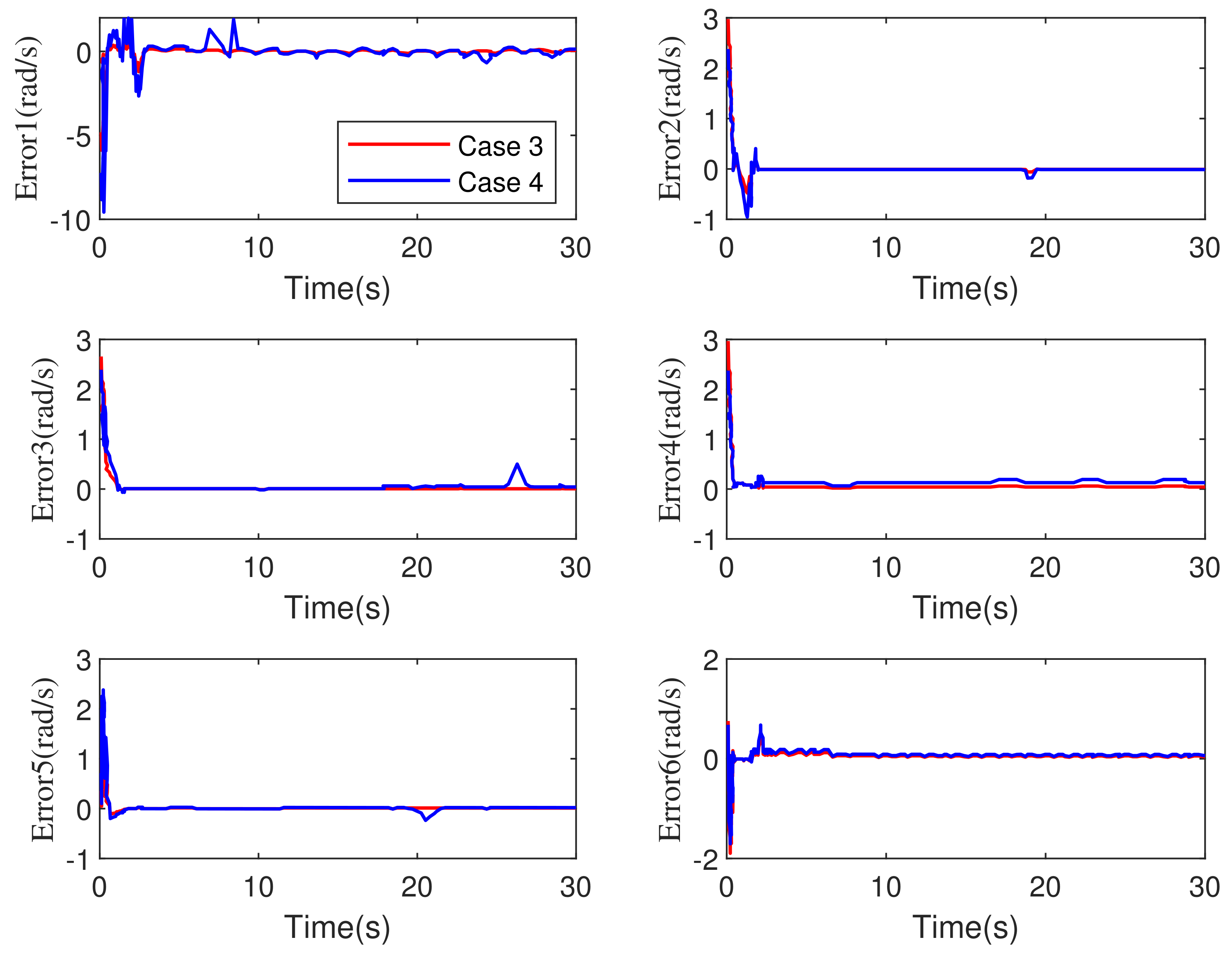
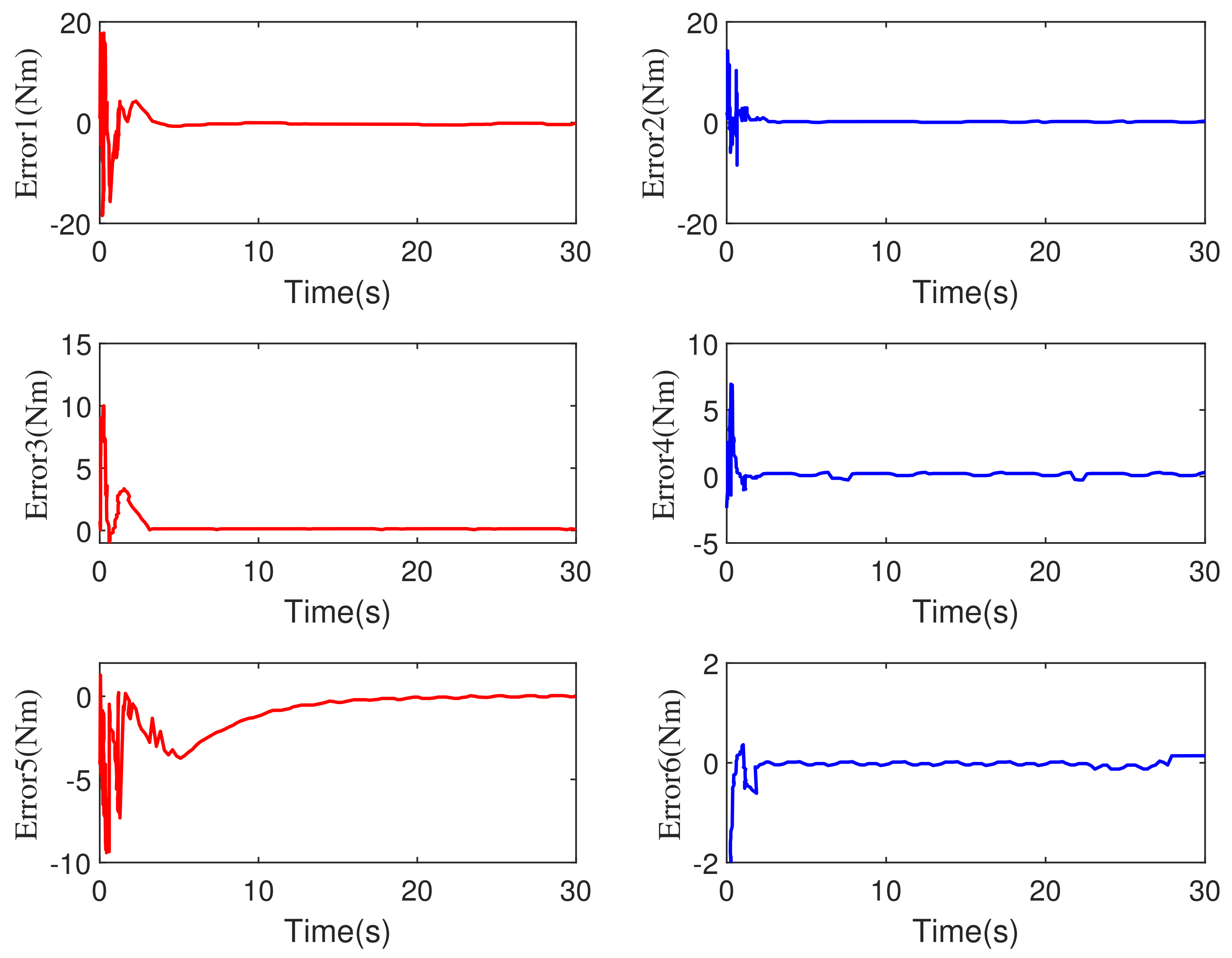
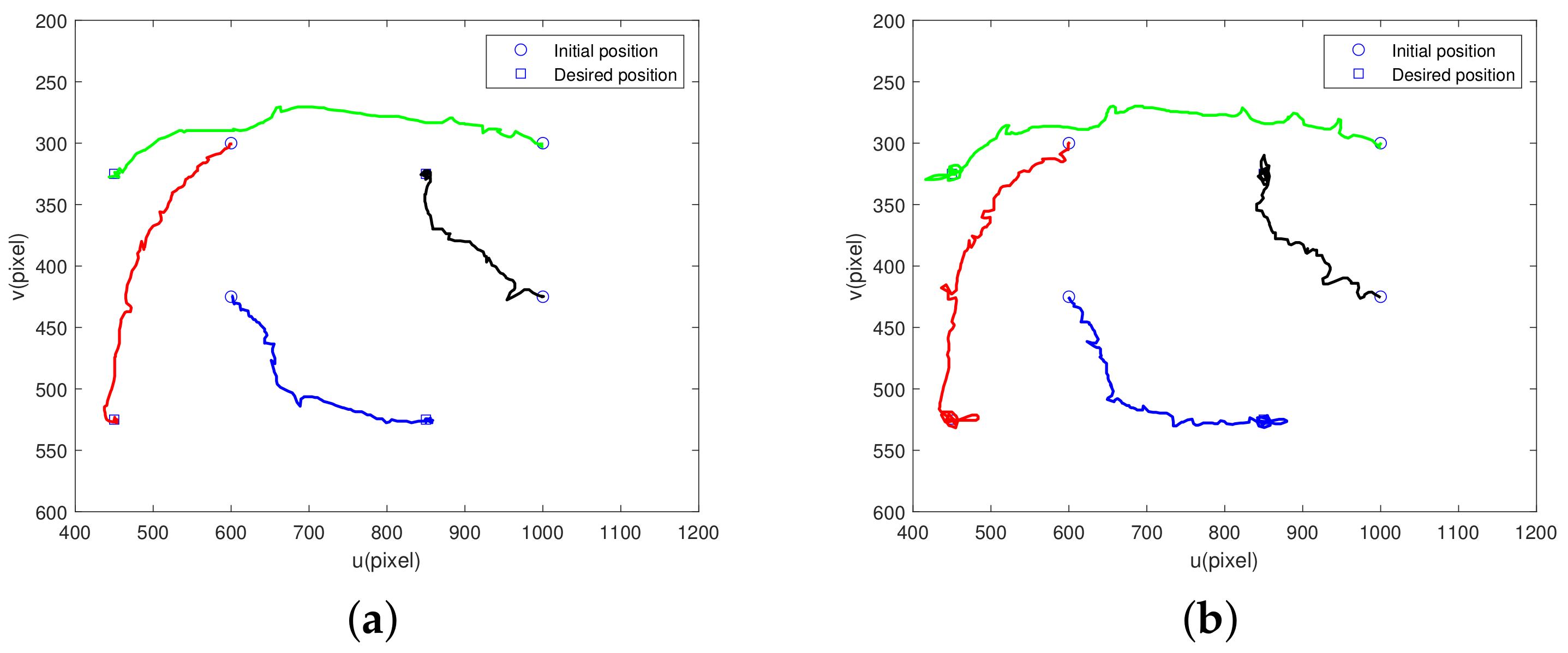
5.2. Comparative Simulations with Time-Varying External Disturbances

The simulation results in the previous section prove that the visual servo controller proposed in this paper can effectively realize the visual servoing by considering system constraints and model uncertainty without measurements of joint velocity. However time-varying disturbances always exist in practical application scenarios, such as joint torque friction. Therefore, we discuss the control effect of the proposed method in visual servoing tasks with time-varying external disturbances in this subsection. The comparative simulations are divided into two parts, which are conducted on the 2-DOF robot manipulator and 6-DOF robot manipulator, respectively. The comparative simulations are carried out between the control strategies proposed in this paper and in [27], which is called Case 4 in this paper.

5.2.1. 2-DOF Robot Manipulator

The parameters of the robot manipulator and camera are the same as in the previous section. The special condition added is that the time-varying external disturbances were given as τ d = 4 sin 3 π 7 t ,   4 sin 3 π 7 t T , which is time-varying.The simulation results are as follows. Figure 9 displays the trajectories of the image features with time-varying external disturbances in Case 3 and Case 4, respectively. The trajectories of Feture Point 1 to Feture Point 4 are shown in red, green, blue and black, respectively. Although there exist fluctuations and turn-back in the trajectories, the image features both respond from the initial positions to the desired positions in Case 3 and Case 4 successfully. However as we can see from Figure 9 and Figure 10, the convergence speed of image errors in Case 3 (about 10 s) is faster than in Case 4 (about 15 s). At the same time, the absolute value of steady-state image errors in Case 3 (about 7 pixels) is smaller than errors in Case 4 (about 18 pixels), as shown in Figure 10. Figure 11 shows the response of the torques under the two strategies. Compared with Case 3, Case 4 brings more frequent ripple to the joint torques as shown in Figure 11, which means a better quality of control. It can also be considered that the input torques are more stable in Case 3. Figure 12 displays the estimation errors of joint velocities in Case 3 and Case 4. It can be seen in Figure 12 that the joint velocities are more accurately estimated by the TOSM observer in Case 3. Figure 13 displays the estimation errors of uncertainties in Case 3. The estimation of uncertainties is given accurately by the TOSM observer in Case 3, then feed back to the controller. While the observer in Case 4 does not have the ability to estimate the uncertainties. As shown in Figure 9, Figure 10, Figure 11, Figure 12 and Figure 13, it can be concluded that the control strategy of Case 3 is superior to that of Case 4 in 2-DOF robot manipulator visual servoing with time-varying external disturbances.

5.2.2. 6-DOF Robot Manipulator

The 6-DOF robot manipulators are most widely used in practical applications. Therefore, it is necessary to verify the effectiveness of the MPC-TOSM method on a 6-DOF robot manipulator. The dynamic parameters and model of 6-DOF robot manipulator are given in [33]. The initial rough camera parameters are given the same settings as above experiments. The Cartesian coordinates of Feture Point 1 to Feture Point 4 that relative to the robot base are 0.6237 , 0.4651 , 2 T m, 0.16 , 0.4651 , 2 T m, 0.6237 , 0.25 , 2 T m, and 0.16 , 0.25 , 2 T m, respectively. The initial 2D coordinates of the image feature points are 600 , 300 T pixels, 1000 , 300 T pixels, 600 , 425 T pixels, and 1000 , 425 T pixels. The desired 2D coordinates of the image-feature points are 450 , 525 T pixels, 450 , 325 T pixels, 850 , 525 T pixels, and 850 , 325 T pixels. The initial states of robot manipulator are chosen as q 1 ( 0 ) = q 2 ( 0 ) = 0 , q 3 ( 0 ) = q 4 ( 0 ) = π 6 , q 5 ( 0 ) = q 6 ( 0 ) = π 12 , q ˙ 1 ( 0 ) = q ˙ 2 ( 0 ) = q ˙ 3 ( 0 ) = q ˙ 4 ( 0 ) = q ˙ 5 ( 0 ) = q ˙ 6 ( 0 ) = 0 . The coordinate transformation matrix of the end-effector framework relative to the camera framework H c e is expressed as
H c e = 1 0 0 0.01 0 1 0 0.02 0 0 1 0.015 0 0 0 1 .
In the experiments, setting the initial rough estimation of camera extrinsic parameter matrix H ^ c e as
H ^ c e = 0.98 0 0.25 0.005 0 0.96 0 0 0 0 0.95 0.01 0 0 0 1 .
The parameters in the third-order sliding mode are chosen as σ 1 = 3 L 1 / 3 , σ 2 = 2 L 2 / 3 , σ 3 = 2 L , with L = 6 . The parameters in the MPC are chosen as Q F = 25 I 8 × 8 , Q G = 0.2 I 6 × 6 , and R = 1 I 6 × 6 , N p = 4 , and N c = 2 . The minimum and maximum torques of the actuator are −80 Nm and 80 Nm. The system uncertainty was given as τ d =   5 sin 2 π 5 t ,   5 sin 2 π 5 t ,   2 sin 2 π 5 t ,   sin 2 π 5 t ,   sin 2 π 5 t ,   sin 2 π 5 t T , which is time-varying.
The simulation results are given as follows:
Figure 14 displays the trajectories of image features in Case 3 and Case 4 with time-varying external disturbances, respectively. The trajectories of Feture Point 1 to Feture Point 4 are shown in red, green, blue and black, respectively. Although there exist fluctuations and turn-back in the trajectories, the image features both respond from the initial positions to the desired positions successfully in Case 3 and Case 4. However as we can see from Figure 14 and Figure 15, the convergence speed of image errors in Case 3(about 8s)is faster than in Case 4 (about 10s). At the same time, the absolute value of steady-state image errors in Case 3 (about 10 pixels) is smaller than errors in Case 4 (about 20 pixels), as shown in Figure 14 and Figure 15. Figure 16 shows the response of the torques under the two strategies. Compared with Case 3, Case 4 brings more frequent ripple to the joint torques as shown in Figure 16. It can also be considered that the input torques are more stable in Case 3. Figure 17 displays the estimation errors of joint velocities with time-varying external disturbances in Case 3 and Case 4. It can be seen that the joint velocities are estimated more accurately by the TOSM observer in Case 3. Figure 18 displays the estimation errors of uncertainties with time-varying external disturbances in Case 3. The estimation of uncertainties is given accurately by the TOSM observer in Case 3, then fed back to the controller. According to Figure 14, Figure 15, Figure 16, Figure 17 and Figure 18, it can be concluded that the control strategy of Case 3 is superior to that of Case 4 in 6-DOF robot manipulator visual servoing.
To sum up, according to the simulation results and discussions above, the proposed MPC-TOSM strategy is a satisfactory method to deal with IBVS tasks by considering system constraints, model uncertainty and time-varying external disturbances with joint velocity unknown.

6. Conclusions

For dealing with the image-based visual servoing problem of robot manipulators with model uncertainty, system constraints, unmeasurable joint angles, and time-varying disturbances, a new MPC method on the basis of a third-order sliding-mode (TOSM) observer is presented in this current research. A TOSM observer is designed for evaluating the joint velocity and system centralized uncertainty simultaneously, and feed-forward the estimated value to the model predictive controller. Using an MPC strategy, the optimal input torque is calculated by decreasing the cost function on the basis of image deviation as far as possible while fully considering the visibility constraints and actuator constraints. Simulation results verify the effectiveness of the proposed MPC-TOSM visual servoing control strategy. In planned subsequent work, we will study the visual servoing problem of tracking dynamic feature points and fully consider the time-delay sensitivity of visual feature feedback in the dynamic tracking process.

Author Contributions

Conceptualization, B.L.; Methodology, J.L., X.P., B.L. and J.W.; Formal Analysis, J.L., X.P., B.L. and J.W.; Data Curation, J.L.; Writing—Original Draft Preparation, J.L.; Writing—Review & Editing, J.L., X.P., B.L. and J.W.; Visualization, J.L.; Supervision, B.L.; Project Administration, B.L.; Funding Acquisition, B.L. All authors have read and agreed to the published version of the manuscript.

Funding

This research was funded by Natural Science Foundation of Heilongjiang Province grant number KY10400210217, Fundamental Research Funds for Central Universities grant number 3072020CFT1501 and Fundamental Strengthening Program Technical Field Fund grant number 2021-JCJQ-JJ-0026 .

Institutional Review Board Statement

Not applicable.

Informed Consent Statement

Not applicable.

Data Availability Statement

Not applicable.

Conflicts of Interest

The authors declare no conflict of interest.

References

  1. Wurll, C.; Fritz, T.; Hermann, Y.; Hollnaicher, D. Production logistics with mobile robots. In Proceedings of the ISR 2018; 50th International Symposium on Robotics, Munich, Germany, 20–21 June 2018; pp. 1–6. [Google Scholar]
  2. Madhusanka, B.G.D.A.; Jayasekara, A.G.B.P. Design and development of adaptive vision attentive robot eye for service robot in domestic environment. In Proceedings of the IEEE International Conference on Information and Automation for Sustainability, Galle, Sri Lanka, 16–19 December 2016; pp. 1–6. [Google Scholar]
  3. Cai, K.; Chi, W.; Meng, M.Q. A vision-based road surface slope estimation algorithm for mobile service robots in indoor environments. In Proceedings of the IEEE International Conference on Information and Automation (ICIA), Fujian, China, 11–13 August 2018; pp. 621–626. [Google Scholar]
  4. Gupta, S.; Mishra, S.R.R.S.; Singal, G.; Badal, T.; Garg, D. Corridor segmentation for automatic robot navigation in indoor environment using edge devices. Comput. Netw. 2020, 178, 107374. [Google Scholar] [CrossRef]
  5. Sim, R.; Little, J.J. Autonomous vision-based robotic exploration and mapping using hybrid maps and particle filters. Image Vis. Comput. 2009, 17, 167–177. [Google Scholar] [CrossRef]
  6. Lazar, C.; Burlacu, A. A Control Predictive Framework for Image-Based Visual Servoing Applications. In Proceedings of the The 24th International Conference on Robotics in Alpe-Adria-Danube Region (RAAD), Bucharest, Romania, 6–8 May 2016. [Google Scholar]
  7. Garcia-Aracil, N.; Perez-Vidal, C.; Sabater, J.M.; Morales, R.; Badesa, F.J. Robust and Cooperative Image-Based Visual Servoing System Using a Redundant Architecture. Sensors 2011, 11, 11885–11900. [Google Scholar] [CrossRef] [PubMed]
  8. Parsapour, M.; RayatDoost, S.; Taghirad, H.D. A 3D sliding mode control approach for position based visual servoing system. Sci. Iran. 2015, 22, 844–853. [Google Scholar]
  9. Park, D.-H.; Kwon, J.-H.; Ha, I.-J. Novel position-based visual servoing approach to robust global stability under field-of-view constraint. IEEE Trans. Ind. Electron. 2012, 59, 4735–4752. [Google Scholar] [CrossRef]
  10. Yan, F.; Li, B.; Shi, W.; Wang, D. Hybrid Visual Servo Trajectory Tracking of Wheeled Mobile Robots. IEEE Access 2018, 6, 24291–24298. [Google Scholar] [CrossRef]
  11. Luo, R.C.; Chou, S.C.; Yang, X.Y.; Peng, N. Hybrid Eye-to-hand and Eye-in-hand visual servo system for parallel robot conveyor object tracking and fetching. In Proceedings of the Iecon 2014—40th Annual Conference of the Ieee Industrial Electronics Society, Dallas, TX, USA, 29 October–1 November 2014. [Google Scholar]
  12. Yoshimi, B.H.; Allen, P.K. Alignment using an uncalibrated camera system. IEEE Trans. Robot. Autom. 1995, 11, 516–521. [Google Scholar] [CrossRef]
  13. Wang, H.; Liu, M. Design of robotic visual servo controlbased on neural network and genetic algorithm. Int. J. Autom. Comput. 2012, 9, 24–29. [Google Scholar] [CrossRef]
  14. Zhong, X.; Zhong, X.; Peng, X. Robust Kalman Filtering Cooperated Elman Neural Network Learning for Vision-Sensing-Based Robotic Manipulation with Global Stability. Sensors 2013, 13, 13464–13486. [Google Scholar] [CrossRef]
  15. Yuksel, T. Intelligent visual servoing with extreme learning machine and fuzzy logic. Expert Syst. Appl. 2017, 22, 344–356. [Google Scholar] [CrossRef]
  16. Kang, M.; Chen, H.; Dong, J. Adaptive Visual Servoing with an Uncalibrated Camera UsingExtreme Learning Machine and Q-leaning. Neurocomputing 2020, 22, 384–394. [Google Scholar] [CrossRef]
  17. Zhou, Y.; Zhang, Y.X.; Gao, J.; An, X.M. Visual Servo Control of Underwater Vehicles Based on Image Moments. In Proceedings of the 6th IEEE International Conference on Advanced Robotics and Mechatronics (ICARM), Chongqing, China, 3–5 July 2021. [Google Scholar]
  18. Anwar, A.; Lin, W.; Deng, X.; Qiu, J.; Gao, H. Quality inspection of remote radio units using depth-free image based visual servo with acceleration command. IEEE Trans. 2019, 66, 8214–8223. [Google Scholar] [CrossRef]
  19. Keshmiri, M.; Xie, W.; Ghasemi, A. Visual Servoing Using an Optimized Trajectory Planning Technique for a 4 DOFs Robotic Manipulator. Int. J. Control. Autom. Syst. 2017, 15, 1362–1373. [Google Scholar] [CrossRef]
  20. Wang, J.P.; Liu, A.; Cho, H.S. Direct path planning in image plane and tracking for visual servoing. In Proceedings of the Optomechatronic Systems Control III, Lausanne, Switzerland, 8–10 October 2007. [Google Scholar]
  21. McFadyen, A.; Jabeur, M.; Corke, P. Image-Based Visual Servoing With Unknown Point Feature Correspondence. IEEE Robot. Autom. Lett. 2017, 2, 601–607. [Google Scholar] [CrossRef]
  22. Jin, Z.H.; Wu, J.H.; Liu, A.D.; Zhang, W.A.; Yu, L. Policy-Based Deep Reinforcement Learning for Visual Servoing Control of Mobile Robots With Visibility Constraints. IEEE Trans. Ind. Electron. 2022, 69, 1898–1908. [Google Scholar] [CrossRef]
  23. Wang, Z.; Kim, D.J.; Behal, A. Design of Stable Visual Servoing Under Sensor and Actuator Constraints via a Lyapunov-Based Approach. IEEE Trans. Control. Syst. Technol. 2012, 20, 1575–1582. [Google Scholar] [CrossRef]
  24. Munoz-Benavent, P.; Gracia, L.; Solanes, J.E.; Esparza, A.; Tornero, J. Robust fulfillment of constraints in robot visual servoing. Control. Eng. Pract. 2018, 71, 79–95. [Google Scholar] [CrossRef]
  25. Li, Z.J.; Yang, C.G.; Su, C.Y.; Deng, J.; Zhang, W.D. Vision-Based Model Predictive Control for Steering of a Nonholonomic Mobile Robot. IEEE Trans. Control. Syst. Technol. 2016, 24, 553–564. [Google Scholar] [CrossRef]
  26. Lazar, C.; Burlacu, A. Predictive control strategy for image based visual servoing of robot manipulators. In Proceedings of the 9th WSEAS International Conference on Automation and Information, Bucharest, Romania, 24–26 June 2008. [Google Scholar]
  27. Qiu, Z.J.Z.; Hu, S.Q.; Liang, X.W. Model Predictive Control for Constrained Image-Based Visual Servoing in Uncalibrated Environments. Asian J. Control. 2019, 21, 783–799. [Google Scholar] [CrossRef]
  28. Wang, T.T.; Xie, W.F.; Liu, G.D.; Zhao, Y.M. Quasi-min-max Model Predictive Control for Image-Based Visual Servoing with Tensor Product Model transformation. Asian J. Control. 2015, 17, 402–416. [Google Scholar] [CrossRef]
  29. Gao, J.; Zhang, G.J.; Wu, P.G.; Zhao, X.Y.; Wang, T.H.; Yan, W.S. Model Predictive Visual Servoing of Fully-Actuated Underwater Vehicles with a Sliding Mode Disturbance Observer. IEEE Access 2019, 3, 25516–25526. [Google Scholar] [CrossRef]
  30. Chaumette, F.; Hutchinson, S. Visual servo control. I. Basic approaches. IEEE Robot. Autom. Mag. 2006, 13, 82–90. [Google Scholar] [CrossRef]
  31. Davila, J.; Fridman, L.; Levant, A. Second-order sliding-mode observer for mechanical systems. IEEE Trans. Automat. Contr. 2005, 50, 1785–1789. [Google Scholar] [CrossRef]
  32. Levant, A. Higher-order sliding modes, differentiation and output-feedback control. Int. J. Control. 2003, 76, 924–941. [Google Scholar] [CrossRef]
  33. Universal Robots A/S. Universal Robots Support-Faq. Available online: www.universal-robots.com/how-tos-and-faqs/faq/ur-faq/ (accessed on 20 April 2022).
Figure 1. Eye-in-hand configuration of 2-DOF robot manipulator.
Machines 10 00465 g001
Figure 2. Eye-to-hand configuration of 2-DOF robot manipulator.
Machines 10 00465 g002
Figure 3. The control system architecture.
Machines 10 00465 g003
Figure 4. Trajectories of the image features of comparative simulations with model uncertainty. (a) Trajectories of the image features in Case 1. (b) Trajectories of the image features in Case 2. (c) Trajectories of the image features in Case 3.
Machines 10 00465 g004
Figure 5. Image errors of comparative simulations with model uncertainty. (a) Image errors in Case 1. (b) Image errors in Case 2. (c) Image errors in Case 3.
Machines 10 00465 g005
Figure 6. Torque of the robot manipulator with model uncertainty in Case 2 and Case 3.
Machines 10 00465 g006
Figure 7. Velocity estimation errors with model uncertainty in Case 2 and Case 3.
Machines 10 00465 g007
Figure 8. Uncertainty estimation errors with model uncertainty in Case 2 and Case 3.
Machines 10 00465 g008
Figure 9. Trajectories of the image features of comparative simulations with time-varying external disturbances for the 2-DOF robot manipulator. (a) Trajectories of the image features in Case 3. (b) Trajectories of the image features in Case 4.
Machines 10 00465 g009
Figure 10. Image errors of comparative simulations with time-varying external disturbances for the 2-DOF robot manipulator. (a) Image errors in Case 3 . (b) Image errors in Case 4.
Machines 10 00465 g010
Figure 11. Torque of the 2-DOF robot manipulator in Case 3 and Case 4.
Machines 10 00465 g011
Figure 12. Velocity estimation errors with time-varying external disturbances in Case 3 and Case 4 for the 2-DOF robot manipulator.
Machines 10 00465 g012
Figure 13. Uncertainties estimation errors with time-varying external disturbances in Case 3 for the 2-DOF robot manipulator.
Machines 10 00465 g013
Figure 14. Trajectories of the image features of comparative simulations with time-varying external disturbances for the 6-DOF robot manipulator. (a) Trajectories of the image features in Case 3. (b) Trajectories of the image features in Case 4.
Machines 10 00465 g014
Figure 15. Image errors of comparative simulations with time-varying external disturbances for the 6-DOF robot manipulator. (a) Image errors in Case 3 with time-varying external disturbances. (b) Image errors in Case 4 with time-varying external disturbances.
Machines 10 00465 g015
Figure 16. Torque of the 6-DOF robot manipulator with time-varying external disturbances in Case 3 and Case 4.
Machines 10 00465 g016
Figure 17. Velocity estimation errors with time-varying external disturbances in Case 3 and Case 4 for the 6-DOF robot manipulator.
Machines 10 00465 g017
Figure 18. Uncertainties estimation errors with time-varying external disturbances in Case 3 for the 6-DOF robot manipulator.
Machines 10 00465 g018
Table 1. Parameters of the 2-DOF robot manipulator.
ith Joint l i (m) m i (kg) l c i (m) I i (kgm 2 )
10.1823.90.0911.27
20.154.440.1050.24
Table 2. Initial rough parameters of the 2-DOF robot manipulator.
ith Joint l ^ i (m) m ^ i (kg) l ^ c i (m) I ^ i (kgm 2 )
10.05200.051.0
20.0540.050.2
Table 3. Camera parameters.
Focal Length (m)Coordinates of the Camera Stagnation Point in the Image Frame (pixels)Scaling Factors along u Axis and v Axis (pixels/m)
Real camera parameters0.0005(646, 482)(269,167, 267,778)
Initial rough camera parameters0.0005(500, 500)(250,000, 250,000)
Publisher’s Note: MDPI stays neutral with regard to jurisdictional claims in published maps and institutional affiliations.

