Abstract
The continuity, self-similarity, and self-affinity of a microscopic contact surface can be described by the Weierstrass–Mandelbrot (W–M) function in fractal theory. To address the problems that the existing normal contact load fractal model does not take into account the effect of thermal stress and is not applicable to the temperature variation in the joint surface of the giant magnetostrictive ultrasonic vibration systems, a fractal model of thermal–elastic–plastic contact normal load fractal is established based on fractal theory. The model is an extension of the traditional model in terms of basic theory and application scope, and it takes into account the effects of temperature difference, linear expansion coefficient, fractal dimension, and other parameters. Finally, the effect of the temperature difference at the joint surface on the normal load of the thermoelastic contact is revealed through numerical simulations. The results show that the nonlinearity of the contact stiffness of the thermoelastic joint surface is mainly related to the surface roughness and the fractal dimension, while the effect of the temperature change on the joint surface properties within a certain range is linear.
1. Introduction
The giant magnetostrictive transducer has the advantages of higher energy density, lower sound speed, no overheating failure, fast response speed, and a strong loading force. These characteristics determine the research direction of developing an ultrasonic machining system with high power, large-amplitude, and wide frequency band [1,2]. Rotational ultrasonic vibration processing can be carried out by giant magnetostrictive transducers made from materials with coupled magnetic, electric, elastic, mechanical, and thermal multiphysics fields [3,4,5,6]. When the GMT works in a high-frequency magnetic field, the eddy current loss in the material is tremendous. The existence of an eddy current weakens the magnetic field provided by the drive coil and changes the uniform distribution of the magnetic field. In addition, frequency-related hysteresis and eddy current reduce the energy conversion efficiency of the giant magnetostrictive materials and change the temperature distribution of the transducer. Temperature rise also causes changes in the contact stiffness of each transducer interface, changes the resonant frequency, and decreases the amplitude stability [2,7]. Zhou et al. [2] developed an equivalent dynamics model of a rotating ultrasonic transducer to investigate the effect of the joint surface stiffness between the horn and the preload force mechanism on the amplitude by a nonlinear least-square fitting method. The results showed that the joint stiffness has an important influence on the dynamic characteristics of the ultrasonic vibration system, but the influence of the thermal effect of the internal giant magnetostrictive material on the interface contact stiffness was not considered. Therefore, determining the interface contact stiffness of the ultrasonic vibration system under the thermal effect and predicting the dynamic characteristics of the ultrasonic system under the change in interface stiffness are urgent problems that need to be solved.
The fractal characteristics of rough surfaces have objective uniqueness or scale independence, providing all surface morphology information within all scale ranges on fractal surfaces [8]. Based on the Weierstrass–Mandelbrot function and statistics, the fractal model and statistical model of rough surface contact were established by early scholars. The direct relationship between the actual contact area, contact load force, contact stiffness, and surface deformation in the elastic, plastic, and elastic–plastic stages of rough surface asperity have been studied. However, these contributions are based on the static characteristics of pure mechanical joints [8,9,10,11,12,13,14,15,16,17,18,19,20]. Based on the fractal theory of rough surface and measurement experiments, Kogut and Komvopoulosa [21] yield insight into the influence of rough surface morphology, current, and contact force on electrical contact thermal resistance. The results showed that the actual contact area of the interface plays a decisive role in the influence of electrical contact thermal resistance. Wang and Komvopoulos [22] established the rough surface fractal theory of interface temperature distribution. They studied the relationship between the maximum temperature rise in the fractal surface domain and the real contact area, thermal–mechanical properties, and fractal parameters. Shi et al. [23] numerically simulated the maximum contact temperature at the interface and the temperature distribution in the contact area of the plate at different sliding speeds. Due to the friction heat source, they studied the thermal–mechanical contact characteristics between the elastic–plastic asperity and the rigid plate. Song et al. [24] studied the thermo–mechanical contact responses of a rigid sphere sliding on an elastic–plastic sphere with a radius more significant than that of the rigid sphere using the finite element method. They obtained the transient values of the interface contact force, the maximum temperature rise, and the actual contact area. Horovistiz et al. [25] used the fractal method in tribological phenomena to fractalize the elevation map of sliding surfaces. They proposed a robust method to determine the threshold between the microscopic scale and the macroscopic scale of fractal behavior; the results showed that the fractal dimension data depend on the tribological conditions and the position along the sliding surface, which have research significance for the accurate determination of material surface fractal parameters.
However, these studies were based on traditional pure mechanical models and did not consider the effect of thermal stress. Therefore, the traditional mechanical interface model cannot truly reflect the actual situation of thermal–mechanical products, such as GMTs working in a long-term changing thermal environment. A fractal model of thermal–elastic–plastic contact normal stiffness, taking into account the thermal effect of rough surface, is proposed in this article by using the superposition method based on the normal contact stiffness model of an anisotropic material. The influence of each main parameter on the normal stiffness of thermal–elastic–plastic contact of the joint surface is analyzed. Fractal theory is used to study the contact behavior of rough surfaces. Then, the theoretical model of the thermal–elastic–plastic contact problem of the rough surface is established. This thermo–mechanical contact characteristic of the joint surface can be utilized to improve the structural design of thermo–mechanical products such as GMTs.
2. Materials and Methods
2.1. Fractal Characterization of Surface Morphology
The rough surface has the mathematical characteristics of statistical self-radioactivity and the multiscale fractal. The Weierstrass–Mandelbrot (W–M) function with double independent variables can fully characterize the mathematical characteristics of a rough surface, and its expression is [26]:
where z(x) is the contour height of the asperity; x, y is the coordinate displacement distance; L is the sample length; Ls is the minimum cut-off length; Φ1,n is the random phase; γ is greater than 1 scale parameter, generally γ = 1.5; n is the spatial frequency index; nmax is the maximum frequency index related to the distance cut-off length; M is the number of overlapping uplifts on the structural surface; G is the fractal roughness coefficient determined by frequency; and D (1 < D < 2) is the fractal dimension of the profile.
When M = 1, m = 1, the W–M function that becomes a single independent variable is:
The three-dimensional contact profiler is used to measure the magnetic conductive sheet (MCS) of a GMT (see [7]) with different roughnesses, as shown in Figure 1. The yellow line is the center of the measurement position and is measured at the center. The material is electrical pure iron, the elastic modulus is 195 MPa, Poisson’s ratio is 0.29, the roughness of the measurement sample is 0.356 μm, the minimum sampling distance of the rough surface measuring instrument is 0.25 μm, and the sampling length is 4 mm. The results of D and G can be obtained using the structural function method [27]. The summary data is shown in Table 1.
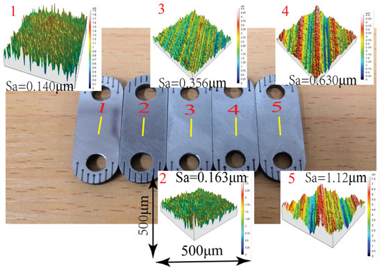
Figure 1.
Micro-surface morphology characteristics of a magnetic conductive sheet.

Table 1.
Fractal parameter values under the same measured surface.
2.2. Fractal Model of Contact Mechanics of Asperity
Figure 2 illustrates the conceptual approach to the contact between a rigid plane and a rough surface. According to Hertz’ contact theory, the contact between two rough -surface asperities is equivalent to the contact between the rigid plane and spherical asperities. To obtain the contact deformation force under a given size, the contact deformation between spherical asperities and a rigid plane must be first obtained. If the maximum contact area of the asperity is , the number of asperities larger than the contact area a can be expressed as N, and the area distribution density of the contact point can be expressed as [27]:
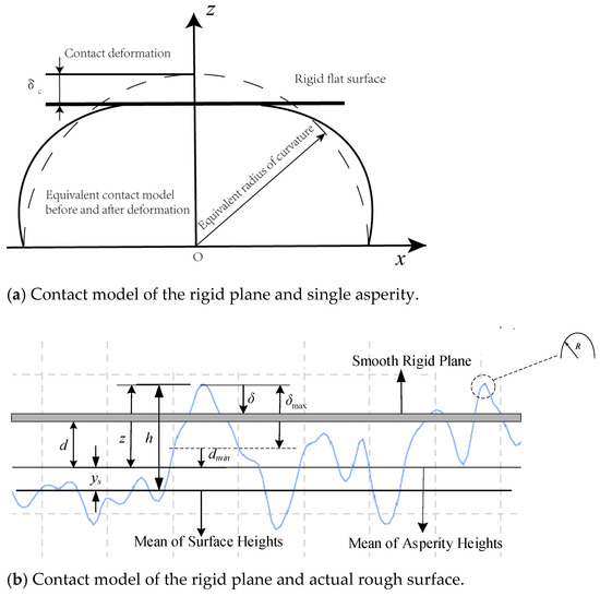
Figure 2.
Schematic diagrams of the geometry of contact; (a) the rigid plane and single asperity (b) the rigid plane and actual rough surface.
According to the area distribution density function of the contact point in Equation (3), the real contact area of the joint surface is derived by:
The interference of an asperity under the force of the rigid plate is equal to the peak-to-valley amplitude of the z(x) function (see Figure 2). is given as [26]:
According to the relationship between the deformation of the asperity and the curvature radius R, considering R≫δ the curvature radius of the asperity is [16]:
To determine the contact parameters of asperity, the contact state of asperity must be determined. According to the finite element results in the literature [9], the deformation of asperity is divided into elastic deformation (), elastic–plastic deformation 1 (), elastic–plastic deformation 2 (), and complete plastic deformation (). is the elastic critical deformation. When the deformation of the asperity exceeds the elastic critical deformation, it begins to yield and enters the elastic–plastic deformation region, which can be expressed as:
where H is the hardness of the soft material, K is the hardness coefficient, K = 0.454 + 0.41, and is Poisson’s ratio.
When , the corresponding contact area is the critical contact area of the asperity . Then, substituting Equations (3) and (4) into Equation (7) gives:
The real contact areas arising in the elastic, elasto–plastic (1), elasto–plastic (2), and fully plastic deformation regimes can be determined if the deformation of asperity for these four deformation regimes are available. Then, the fractal theory of contact area can be obtained in different stages.
If the deformation of the asperity is in the range of (), the elastic contact load and contact stiffness , produced by a sphere with a radius of curvature of R in contact with a rigid plane with an elastic interference, are given based on fractal theory as follows:
If the deformation of the asperity is in the range of (), the contact mechanics model of elastic–plastic deformation zone 1 is expressed in fractal form as:
Moreover, if the deformation of the asperity is in the range of (), the contact mechanics model of elastic–plastic deformation zone 2 is expressed in fractal form as:
When , the contact mode is complete plastic deformation, and the contact mechanics model is expressed in fractal form as:
2.3. Thermal–Mechanical Coupling Contact Interface
We now present a modified asperity contact stiffness model that is similar to the contact mechanics model of asperity in Section 2.2, only because the aggregated heat flow propagates between rough contact interfaces, as shown in Figure 3. Unlike the interface contact model in Section 2.2, which assumes that the asperity is subjected to pure static compressive stress, this model considers contact thermal resistance and the influence of thermal stress on contact deformation when heat flow passes through the contact interface. This model especially considers the influence of thermoelastic deformation. A more practical interface stiffness model of ultrasonic vibration is established by coupling the contact interface’s static stiffness with the interface’s thermal stiffness under static pressure, namely the interface composite stiffness.
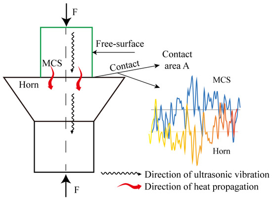
Figure 3.
Ultrasound system–interface stiffness model under thermal effect.
2.3.1. Thermal Contact Resistance of Rough Surface Interface
When the heat flow generated by a magnetostrictive material passes through the rough contact interface of the MCS and the horn, the contact thermal resistance is generated at the interface under the action of the interface contact pressure. Additionally, the contact force between the asperity and the interface is given in Section 2.2 and Section 2.3. Interface contact thermal resistance mainly includes interface material matrix contact thermal resistance, heat flow shrinkage thermal resistance, and interface gap thermal resistance. The contact model of heat flow propagation between the contact interfaces is assumed as follows: the temperature difference between contact interfaces is the same; the heat transfer mode of fluid medium in the contact interface gap is heat conduction, without thermal convection and thermal radiation; the height area distribution function of contact interface asperity obeys the fractal model. Based on the GMT of the ultrasonic machining system, the contact thermal resistance of the material matrix and the contact thermal resistance of the interface gap are negligible compared with the heat flux shrinkage thermal resistance. Therefore, we only considered the heat flux shrinkage thermal resistance.
Microscopically, the rough interface contact between the MCS and the horn manifests as mutual contact between the asperities, which is further manifested as peak-to-peak contact between the asperities. We did not consider other contact types, such as side contact or mixed contact. When the heat flow propagates at two rough contact interfaces, it produces thermal shrinkage, namely shrinkage thermal resistance. The degree of heat flow contraction is inversely proportional to the number of contacted asperities. According to the classical truncated cone contact model, the thermal shrinkage resistance at the contact point of a single asperity can be expressed as [28]:
where b and c are the radius of the heat flow channel and the contact point, respectively, which can be solved by the equation ; is the dimensionless real contact area; is the interface shrinkage, which can be approximately expressed as ; is the equivalent thermal conductivity, which can be calculated by , where and are the thermal conductivity of the two contact materials, respectively. Substituting contact radius R of asperity into Equation (19), contact thermal conductance of asperity becomes:
Then, the contact thermal conductivity of asperity in the plastic stage, elastic–plastic stage 1 and 2, and elastic deformation stage can be further expressed as:
where , , , and represent the contact area of the asperity in the elastic, elastic–plastic 1 and 2, and plastic stages, respectively, which can be obtained based on the fractal model of contact mechanics in each stage.
According to the statistical principle, the contact thermal conductivity of the real area of the joint surface can be obtained based on the idea of a single microconvex body to the entire interface:
2.3.2. Composite Stiffness
A single asperity’s steady thermoelastic deformation under thermal effect is analyzed based on thermoelastic strain. Although the thermal strain of a contact interface can also be accurately expressed from the perspective of the one-dimensional height of the asperity, it requires more assumptions and more complex mathematical calculations. At the same time, in order to ensure the consistency and universality of the calculation of the normal contact force in Section 2.2, the calculation of the thermal–elastic force is simplified, that is, the contact thermal–elastic deformation force between the asperities can be expressed as:
where α is the linear expansion coefficient of the material, and E is the equivalent elastic modulus; is the temperature difference with the environment; and is the actual deformation area of elastic deformation stage. Combined with (10), the normal force of a single asperity containing thermal stress in the elastic deformation stage can be obtained as follows:
In Equation (27), the value in the elastic deformation regime can be determined by differentiating Equation (28), which produces:
where the former is the static elastic stiffness of the mechanical load, and the latter is the elastic deformation stiffness of the thermal response, namely, the thermal stiffness. According to statistics from local to global, the thermal–elastic–plastic normal stiffness of the joint surface is composite stiffness. Regarding coupled thermal stiffness, we take into account only the elastic stage of deformation without considering the thermal effects of other stages of deformation. We also ignore the impact of coupled thermal stiffness on plastic deformation. This is very important. Although it is rough, it dramatically reduces the complexity and improves computational efficiency. The thermal stiffness of the joint surface can be expressed as:
After dimensionless processing, (29) is expressed as:
By applying Equations (3), (10) and (18), the deformation force and contact stiffness function from a single asperity to the whole interface based on statistical principles can be deduced. After dimensionless processing, the total contact force containing thermoelastic stress can be calculated as follows when the fractal dimension D is not equal to 1.5:
At a given mean surface separation distance, when the fractal dimension D is equal to 1.5, the total contact force containing thermoelastic stress can be calculated as follows:
Then, the total contact stiffness of the whole joint surface containing thermal stiffness can be unified as:
where is the nominal contact area, is the real contact area, is the critical contact area, and the dimensionless processing can be obtained by:
3. Results and Discussion
Numerical Simulation
Regarding the effects of temperature on the elastic modulus E and linear expansion coefficient, it is necessary to take corresponding values according to the variable physical parameters of related materials. The results, K*, as shown in Figure 4 are expressed as a function of the dimensionless temperature change (). D is taken as 1.1–1.9, G is taken as 10−10, 10−11, and 10−12. As shown in the Figure 4, when the modified fractal model considering temperature deformation is considered, the dimensionless contact stiffness K* increases with the increase in and presents a robust linear relationship. For the same change temperature, K* decreases with the increase in G within a specific range, and this change becomes particularly significant at G = 10−12, while it becomes an inclined line with a small slope at G = 10−10 . The increase in G indicates the increase in roughness of a rough surface, and the elastic contact percentage of the thermal effect between rough contact surfaces decreases, indicating that the minor roughness of the joint surface has a significant influence on the thermal effect of the interface.
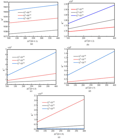
Figure 4.
Influence of length scale parameter G* on -K* curve; (a) D = 1.1 (b) D = 1.3 (c) D = 1.5 (d) D = 1.7 (e) D = 1.9.
Figure 5 shows the variation in with under different D and G when the dimensionless temperature is 300. The dimensional normal contact stiffness of the joint surface, considering the thermal effect, increases with the increase in the dimensional normal total contact load ; that is, the normal deformation of the joint surface, the normal contact load, and the normal contact stiffness are proportional. In the range of fractal dimension D = 1.1~1.5, in the small range of the contact force, and show a significant nonlinear relationship, as shown in Figure 5a–d, that is, strong interface nonlinearity. The contact force and stiffness in this range have an essential influence on the stability of the ultrasonic vibration system. In the design, the influence of the nonlinearity of this process on the stability of ultrasonic vibration should be avoided. When , the linear relationship of interface characteristic parameters is increasingly prominent, as shown in Figure 5e,f. This range is beneficial to the stability of the ultrasonic vibration system due to the linear interface characteristics. In short, under the thermal effect of a specific temperature, the actual elastic contact area and normal contact stiffness of the rough contact interface increase with the increase in the contact load.
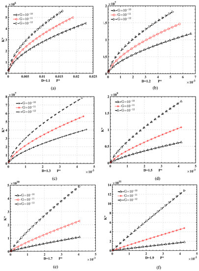
Figure 5.
Influence of length scale parameter G* on -K* curve with = 300; (a) D = 1.1 (b) D = 1.2 (c) D = 1.3 (d) D = 1.5 (e) D = 1.7 (f) D = 1.9.
Figure 6 is the influence curve of fractal dimension D on normal contact stiffness K* when = 300, . As shown in the figure, within a specific range of contact force (), the curve shows a nonlinear solid relationship. When , the linear interface relationship is apparent, which is consistent with the corresponding relationship in Figure 5. The nonlinear interface relationship is again verified.
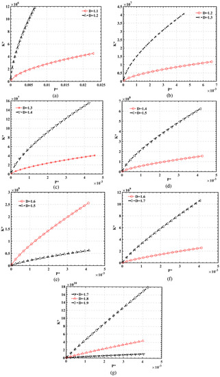
Figure 6.
Influence of fractal dimensions D on -K* curve with = 300; (a) D = 1.1, 1.2 (b) D = 1.2, 1.3 (c) D = 1.3, 1.4 (d) D = 1.4, 1.5 (e) D = 1.5, 1.6 (f) 1.6, 1.7 (g) 1.7, 1.8, 1.9.
4. Conclusions
In this study, the composite contact stiffness model of an ultrasonic vibration system under a preload due to the thermal effect was established. The following conclusions were obtained:
- The change in interface stiffness under the thermal effect increases with temperature, and the linear relationship between the temperature and interface stiffness is apparent. Therefore, a reasonable cooling method must be adopted in the GMT system in the operation process so that the system can work in a reasonable temperature range.
- When , the interface nonlinearity is pronounced. For the same change temperature, K* decreases with the increase in G within a specific range, and this change becomes particularly significant at .
- The proposed interface thermal stiffness contact model can provide theoretical guidance for the study and optimal design of nonlinear dynamic characteristics of ultrasonic vibration systems (e.g., rotating giant magnetostrictive transducers) or other thermal products from the point of view of the contact interface.
Author Contributions
Conceptualization, Y.C.; methodology, P.L.; software, J.S; validation, J.S.; formal analysis, Y.C.; investigation, J.S., M.S. and L.S.; resources, P.L.; data curation, Y.C.; writing—original draft preparation, Y.C.; writing—review and editing, P.L.; visualization, J.S.; supervision, L.S.; project administration, P.L.; funding acquisition, P.L. All authors have read and agreed to the published version of the manuscript.
Funding
This research was supported by the National Natural Science Foundation of China (Grant Number: 52075439), the Shanxi Province Natural Science Foundation of China (Grant Number: 2022QFY01-01), and the Doctoral innovation fund of Xi’an University of Technology (Grant Number: 252072104).
Institutional Review Board Statement
Not applicable.
Informed Consent Statement
Not applicable.
Data Availability Statement
Data are contained within the article as figures and tables.
Conflicts of Interest
The authors declare no conflict of interest.
Nomenclature
| random phase | |
| n | spatial frequency index |
| M | number of overlapping uplifts on the structural surface |
| G | fractal roughness coefficient determined by frequency |
| L | sample length |
| area distribution density of the contact point | |
| N | number of asperities larger than contact area a |
| real contact area of joint surface | |
| peak-to-valley amplitude of the z(x) function | |
| R | curvature radius of the asperity |
| elastic critical deformation | |
| K | the hardness coefficient |
| Poisson’s ratio | |
| critical contact area of asperity | |
| elastic contact load | |
| contact mechanics of elastic–plastic deformation zone 1 | |
| contact mechanics of elastic–plastic deformation zone 2 | |
| contact mechanics of complete plastic deformation | |
| thermal shrinkage resistance at contact point of a single asperity | |
| contact thermal conductance of asperity | |
| contact thermal conductivity of real area of joint surface | |
| normal load caused by thermal stress | |
| normal force of a single asperity containing thermal stress in elastic deformation stage | |
| total contact force containing thermoelastic stress | |
| total contact stiffness of whole joint surface containing thermal stiffness | |
| nominal contact area |
References
- Ma, K.; Wang, J.; Zhang, J.; Feng, P.; Yu, D.; Ahmad, S. A highly temperature-stable and complete-resonance rotary giant magnetostrictive ultrasonic system. Int. J. Mech. Sci. 2022, 214, 106927. [Google Scholar] [CrossRef]
- Zhou, H.; Zhang, J.; Feng, P.; Yu, D.; Wu, Z. An amplitude prediction model for a giant magnetostrictive ultrasonic transducer. Ultrasonics 2020, 108, 106017. [Google Scholar] [CrossRef] [PubMed]
- Zhan, Y.-S.; Lin, C.-H. A Constitutive Model of Coupled Magneto-thermo-mechanical Hysteresis Behavior for Giant Magnetostrictive Materials. Mech. Mater. 2020, 148, 103477. [Google Scholar] [CrossRef]
- Wang, T.-Z.; Zhou, Y.-H. Nonlinear dynamic model with multi-fields coupling effects for giant magnetostrictive actuators. Int. J. Solids Struct. 2013, 50, 2970–2979. [Google Scholar] [CrossRef]
- Xiao, Y.; Gou, X.F.; Zhang, D.G. A one-dimension nonlinear hysteretic constitutive model with elasto-thermo-magnetic coupling for giant magnetostrictive materials. J. Magn. Magn. Mater. 2017, 441, 642–649. [Google Scholar] [CrossRef]
- Zhan, Y.-S.; Lin, C.-H. Micromechanics-based constitutive modeling of magnetostrictive 1–3 and 0–3 composites. Compos. Struct. 2021, 260. [Google Scholar] [CrossRef]
- Li, P.; Liu, Q.; Zhou, X.; Xu, G.; Li, W.; Wang, Q.; Yang, M. Effect of Terfenol-D rod structure on vibration performance of giant magnetostrictive ultrasonic transducer. J. Vib. Control 2020, 27, 573–581. [Google Scholar] [CrossRef]
- Chen, Y.; Zhang, X.; Wen, S.; Lan, G. Fractal Model for Normal Contact Damping of Joint Surface Considering Elastoplastic Phase. J. Mech. Eng. 2019, 55, 58–68. [Google Scholar]
- Kogut, L.; Etsion, I. Elastic-Plastic Contact Analysis of a Sphere and a Rigid Flat. J. Appl. Mech. 2002, 69, 657–662. [Google Scholar] [CrossRef]
- Kogut, L.; Etsion, I. A Finite Element Based Elastic-Plastic Model for the Contact of Rough Surfaces. Tribol. Trans. 2003, 46, 383–390. [Google Scholar] [CrossRef]
- Brake, M.R. An analytical elastic-perfectly plastic contact model. Int. J. Solids Struct. 2012, 49, 3129–3141. [Google Scholar] [CrossRef]
- Xu, C.; Wang, D. An Improved Analytical Model for Normal Elastic-Plastic Contact of Rough Surfaces. J. Xi’an Jiaotong Univ. 2014, 48, 115–121. [Google Scholar]
- Jiang, S.; Zheng, Y.; Zhu, H. A Contact Stiffness Model of Machined Plane Joint Based on Fractal Theory. J. Tribol.-Trans. Asme 2010, 132, 011401. [Google Scholar] [CrossRef]
- Raffa, M.L.; Lebon, F.; Vairo, G. Normal and tangential stiffnesses of rough surfaces in contact via an imperfect interface model. Int. J. Solids Struct. 2016, 87, 245–253. [Google Scholar] [CrossRef]
- Liu, W.; Yang, J.; Xi, N.; Shen, J.; Li, L. A study of normal dynamic parameter models of joint interfaces based on fractal theory. J. Adv. Mech. Des. Syst. Manuf. 2015, 9, JAMDSM0070. [Google Scholar] [CrossRef]
- Liou, J.L.; Tsai, C.M.; Lin, J.-F. A microcontact model developed for sphere- and cylinder-based fractal bodies in contact with a rigid flat surface. Wear 2010, 268, 431–442. [Google Scholar] [CrossRef]
- Liou, J.L.; Lin, J.F. A modified fractal microcontact model developed for asperity heights with variable morphology parameters. Wear 2010, 268, 133–144. [Google Scholar] [CrossRef]
- Wang, Z.; Liu, X. Model for Elastic-Plastic Contact between Rough Surfaces. J. Tribol. 2018, 140, 051402. [Google Scholar] [CrossRef]
- He, L.G.; Zuo, Z.X.; Xiang, J.H. Normal Contact Stiffness Fractal Model Considering Asperity Elastic-Plastic Transitional Deformation Mechanism of Joints. J. Shanghai Jiaotong Univ. 2015, 49, 116–121. [Google Scholar]
- Li, L.; Liang, X.; Xing, Y.Z.; Yan, D.; Wang, G. Measurement of Real Contact Area for Rough Metal Surfaces and the Distinction of Contribution From Elasticity and Plasticity. J. Tribol. 2021, 143, 071501. [Google Scholar] [CrossRef]
- Kogut, L.; Komvopoulos, K. Electrical contact resistance theory for conductive rough surfaces separated by a thin insulating film. J. Appl. Phys. 2004, 95, 576–585. [Google Scholar] [CrossRef]
- Wang, S.; Komvopoulos, K. Closure to “Discussion of ‘A Fractal Theory of the Interfacial Temperature Distribution in the Slow Sliding Regime: Part I—Elastic Contact and Heat Transfer Analysis’” (1994, ASME J. Tribol., 116, p. 822). J. Tribol. 1994, 116, 822–823. [Google Scholar] [CrossRef][Green Version]
- Shi, X.; Wu, A.; Jin, C.; Qu, S. Thermomechanical modeling and transient analysis of sliding contacts between an elastic–plastic asperity and a rigid isothermal flat. Tribol. Int. 2015, 81, 53–60. [Google Scholar] [CrossRef]
- Song, W.; Li, L.; Ovcharenko, A.; Talke, F.E. Thermo-mechanical contact between a rigid sphere and an elastic–plastic sphere. Tribol. Int. 2016, 95, 132–138. [Google Scholar] [CrossRef]
- Horovistiz, A.; Laranjeira, S.; Davim, J.P. 3-D reconstruction by extended depth-of-field in tribological analysis: Fractal approach of sliding surface in Polyamide66 with glass fiber reinforcement. Polym. Test. 2019, 73, 178–185. [Google Scholar] [CrossRef]
- Yan, W.; Komvopoulos, K. Contact analysis of elastic-plastic fractal surfaces. J. Appl. Phys. 1998, 84, 3617–3624. [Google Scholar] [CrossRef]
- Majumdar, A.; Bhushan, B. Fractal Model of Elastic-Plastic Contact Between Rough Surfaces. J. Tribol. 1991, 113, 1–11. [Google Scholar] [CrossRef]
- Cooper, M.G.; Mikic, B.B.; Yovanovich, M.M.; Transfer, M. Thermal Contact Conductance. Int. J. Heat Mass Transf. 1969, 12, 279–300. [Google Scholar] [CrossRef]
Publisher’s Note: MDPI stays neutral with regard to jurisdictional claims in published maps and institutional affiliations. |
© 2022 by the authors. Licensee MDPI, Basel, Switzerland. This article is an open access article distributed under the terms and conditions of the Creative Commons Attribution (CC BY) license (https://creativecommons.org/licenses/by/4.0/).