
Modelling Particle Motion during High-Voltage Electrostatic Abrasive Implantation Based on Multi-Physics Field Coupling


Abstract
:1. Introduction
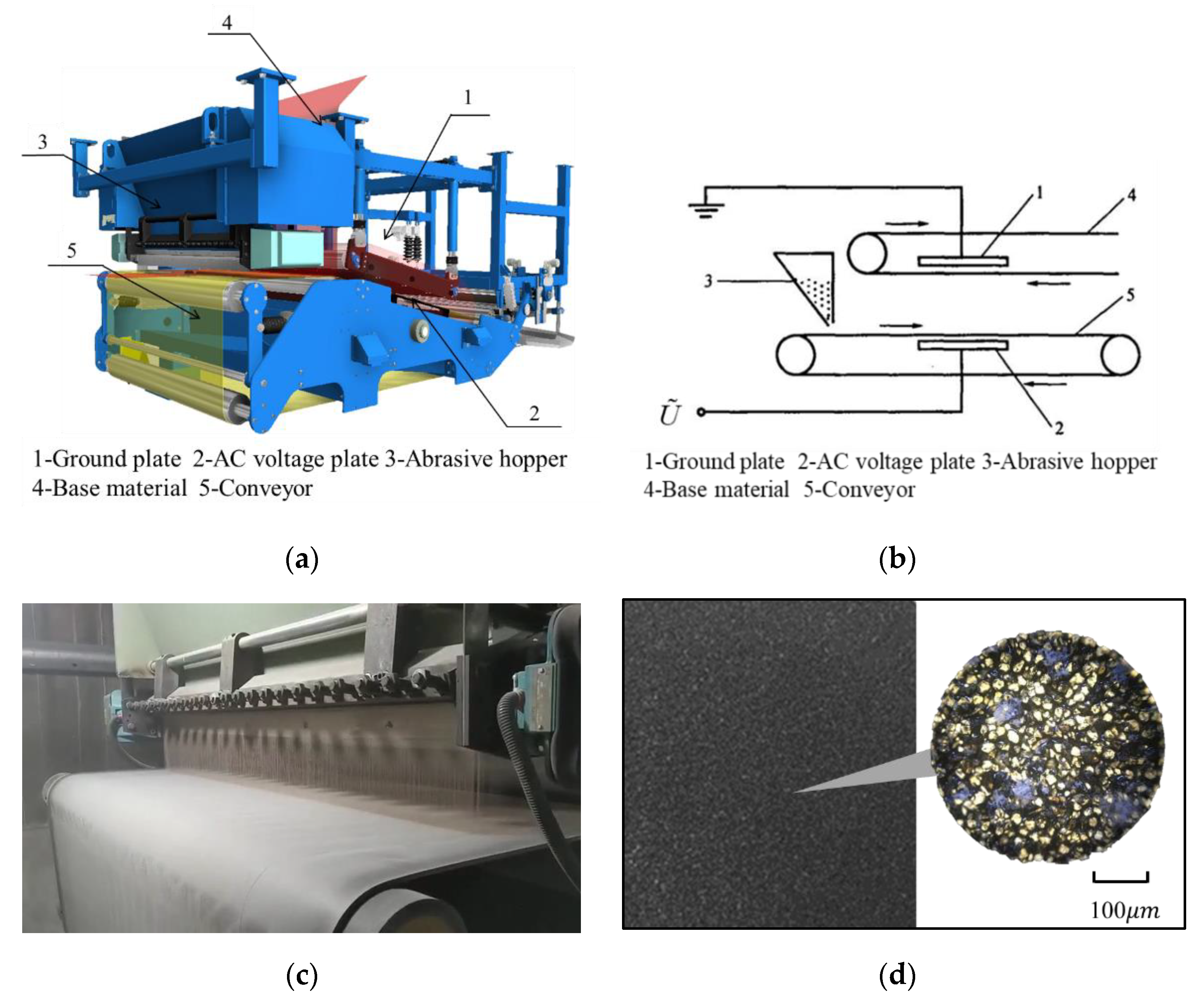
2. Model and Method
2.1. Governing Equations
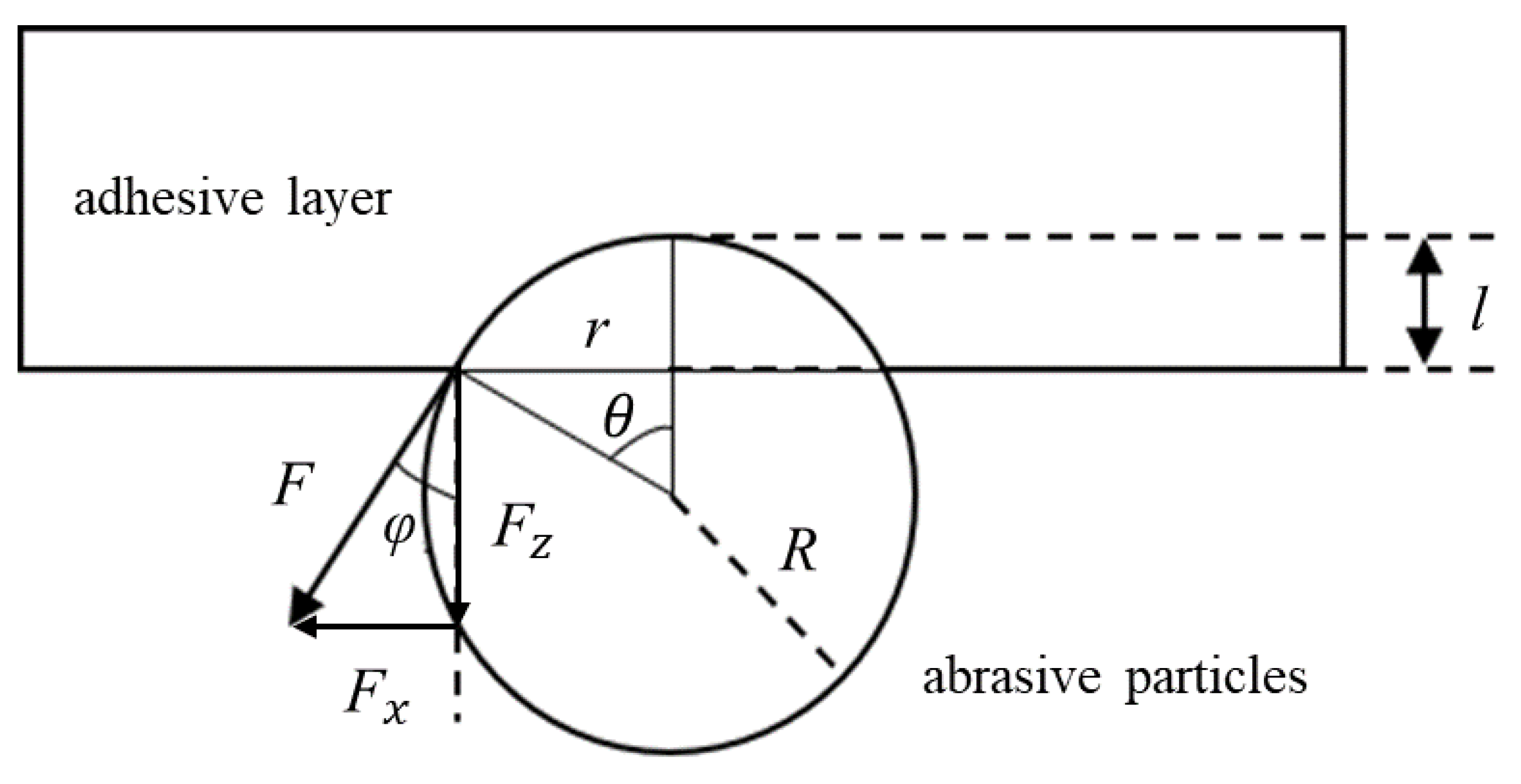
- F the adhesive force on abrasive particles, N;
- μ1 the kinematic viscosity of the adhesive, Pa·s;
- A the area of contact between abrasive and adhesive layer, m2;
- u the abrasive velocity, m/s;
- l the depth of abrasive into the adhesive layer, m.
2.2. Multi-Physics Modelling
2.2.1. Mechanical Model
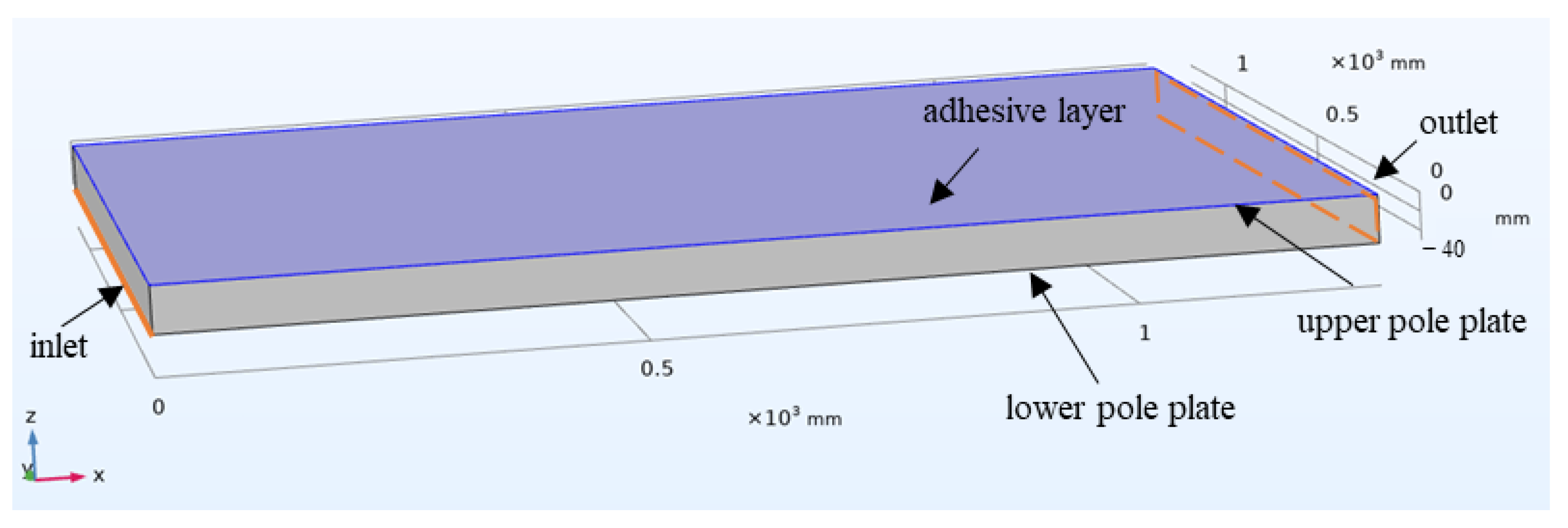
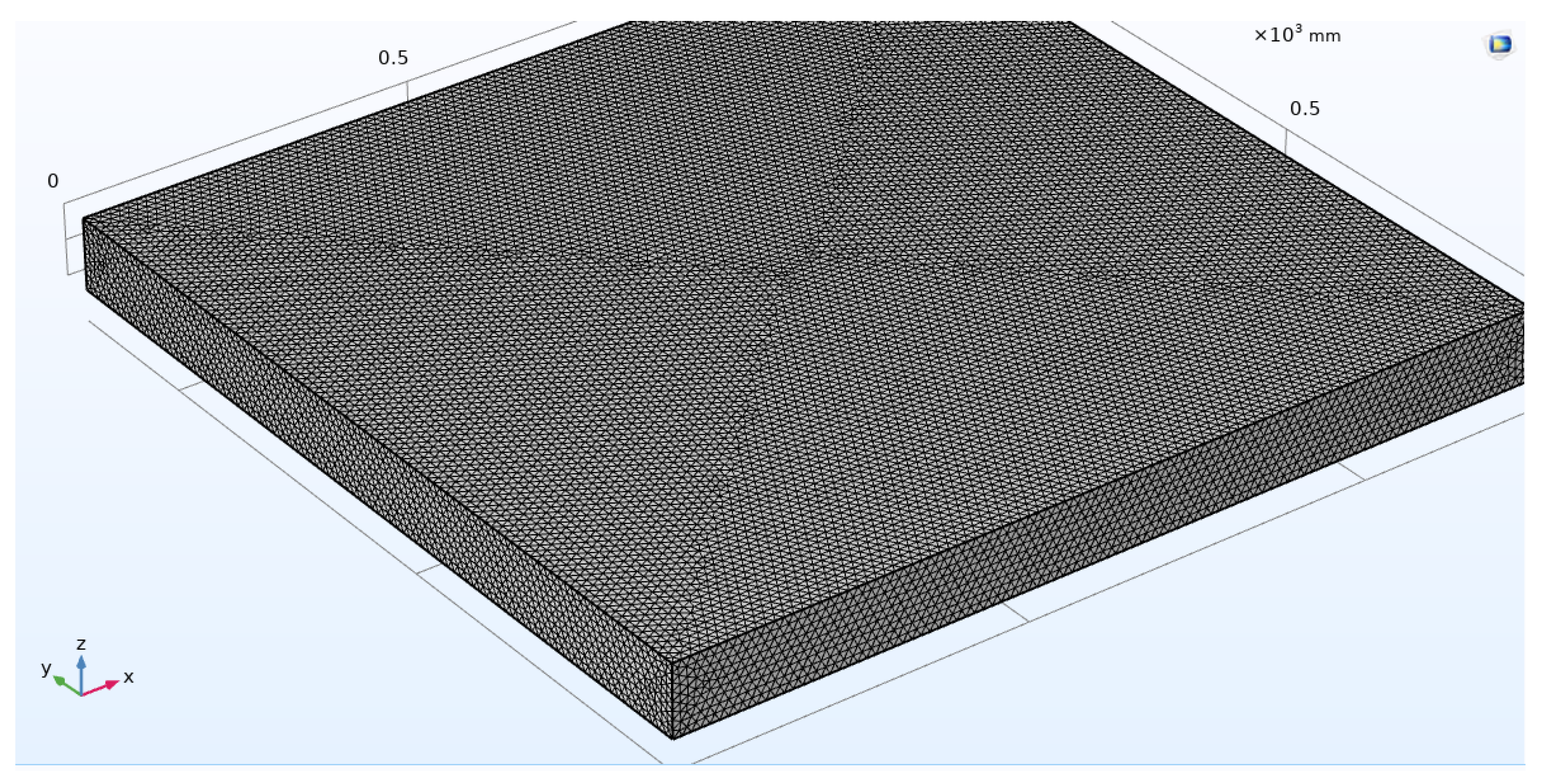
2.2.2. Field Model
3. Simulation and Experiments
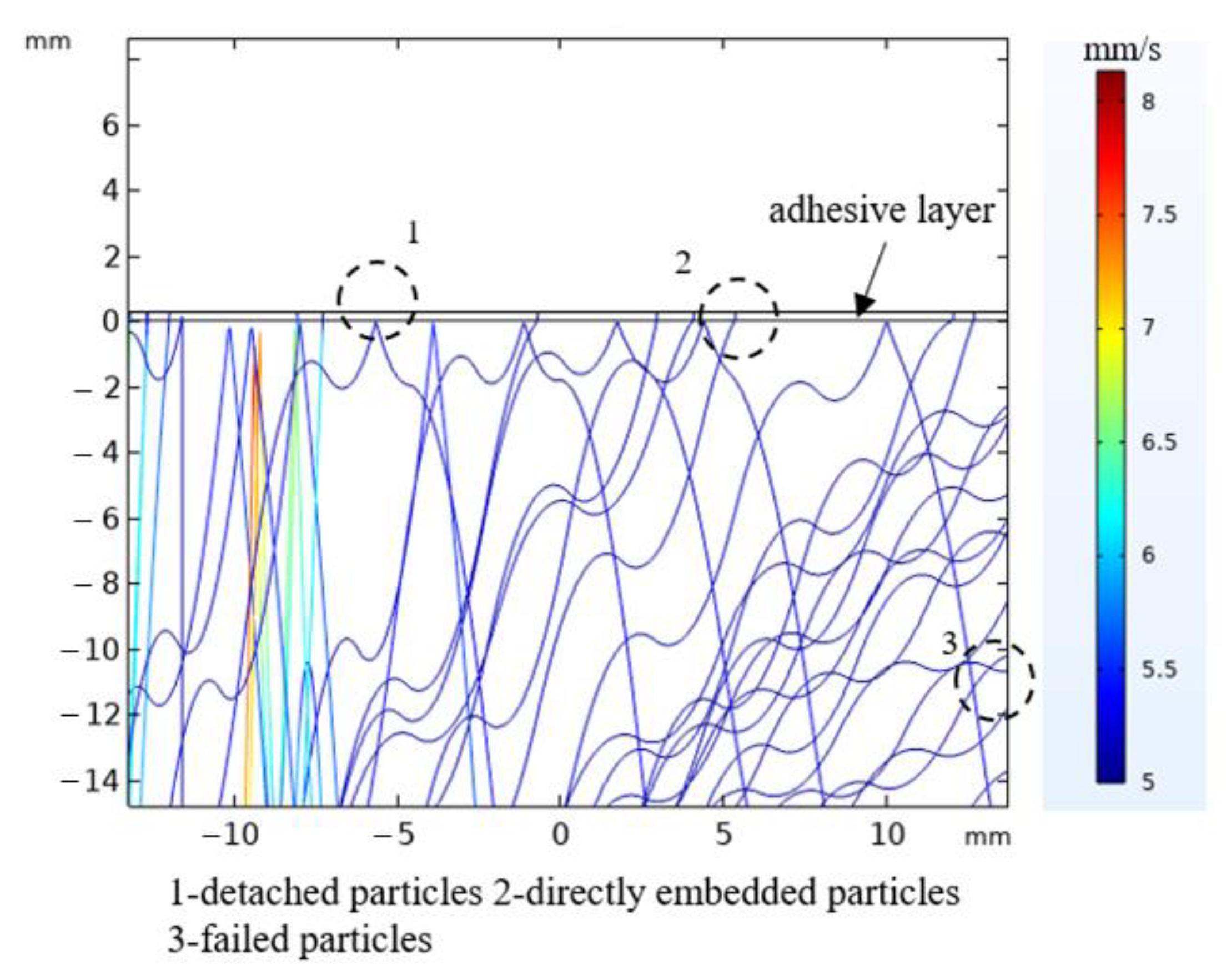
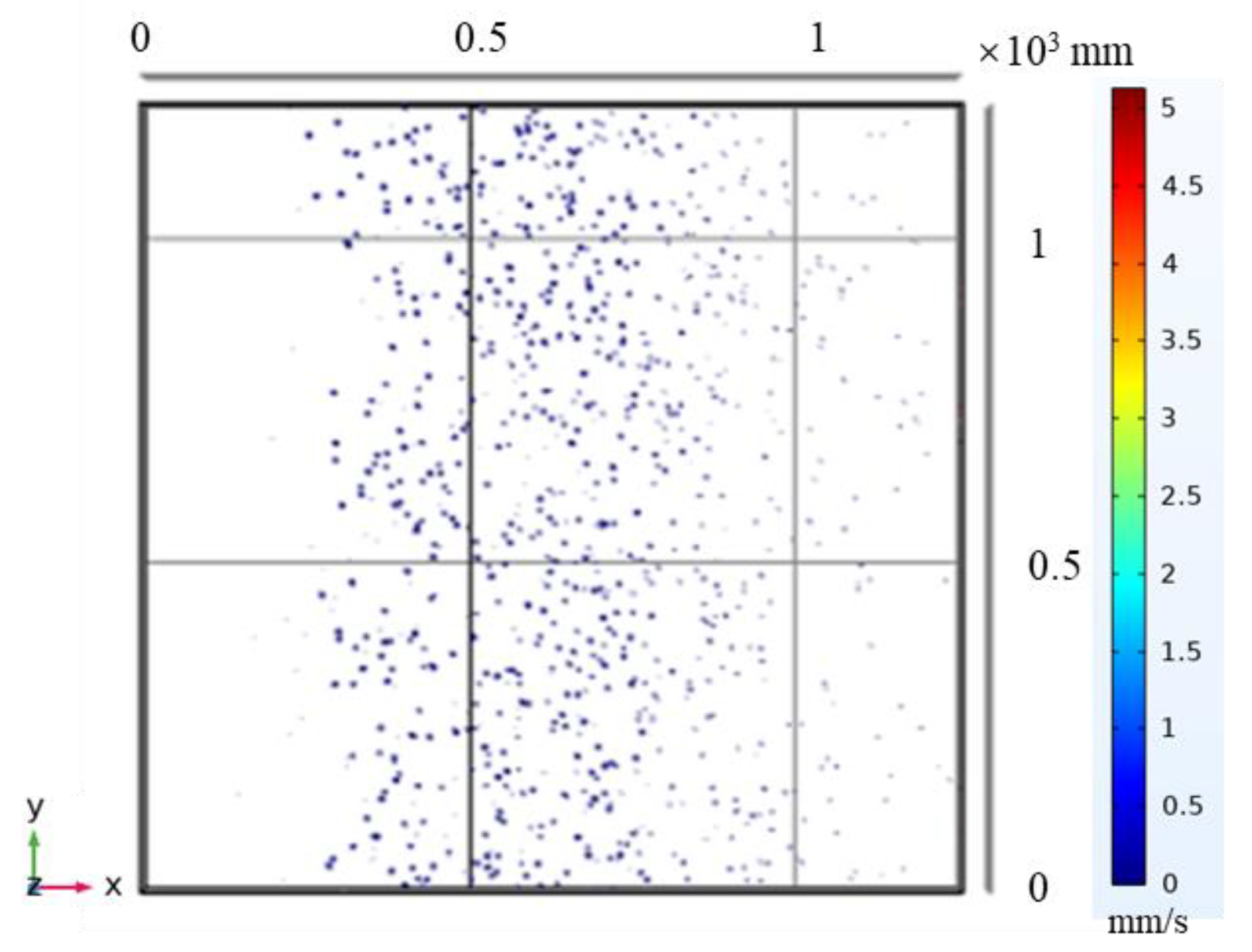
3.1. Simulation Results
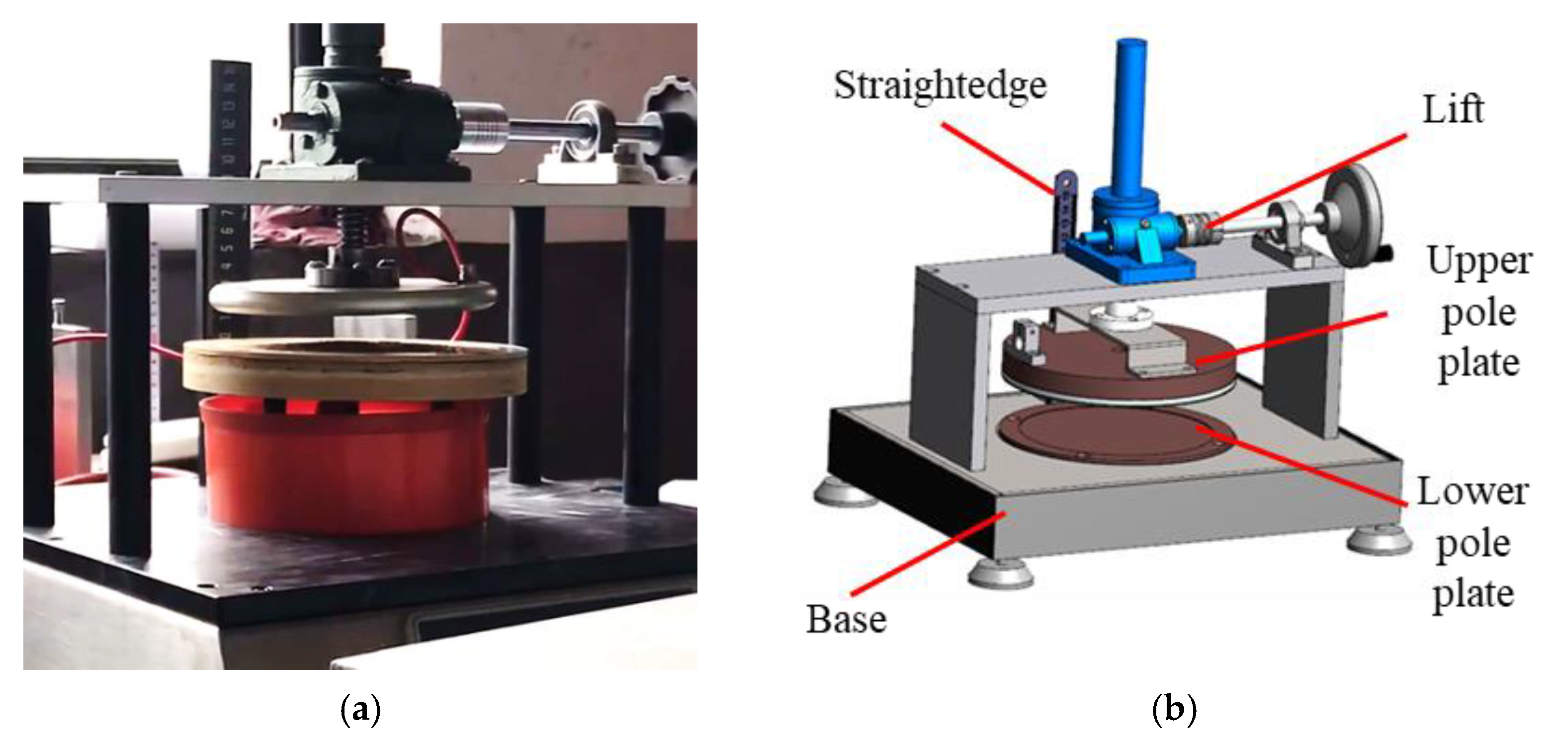
3.2. Experiments
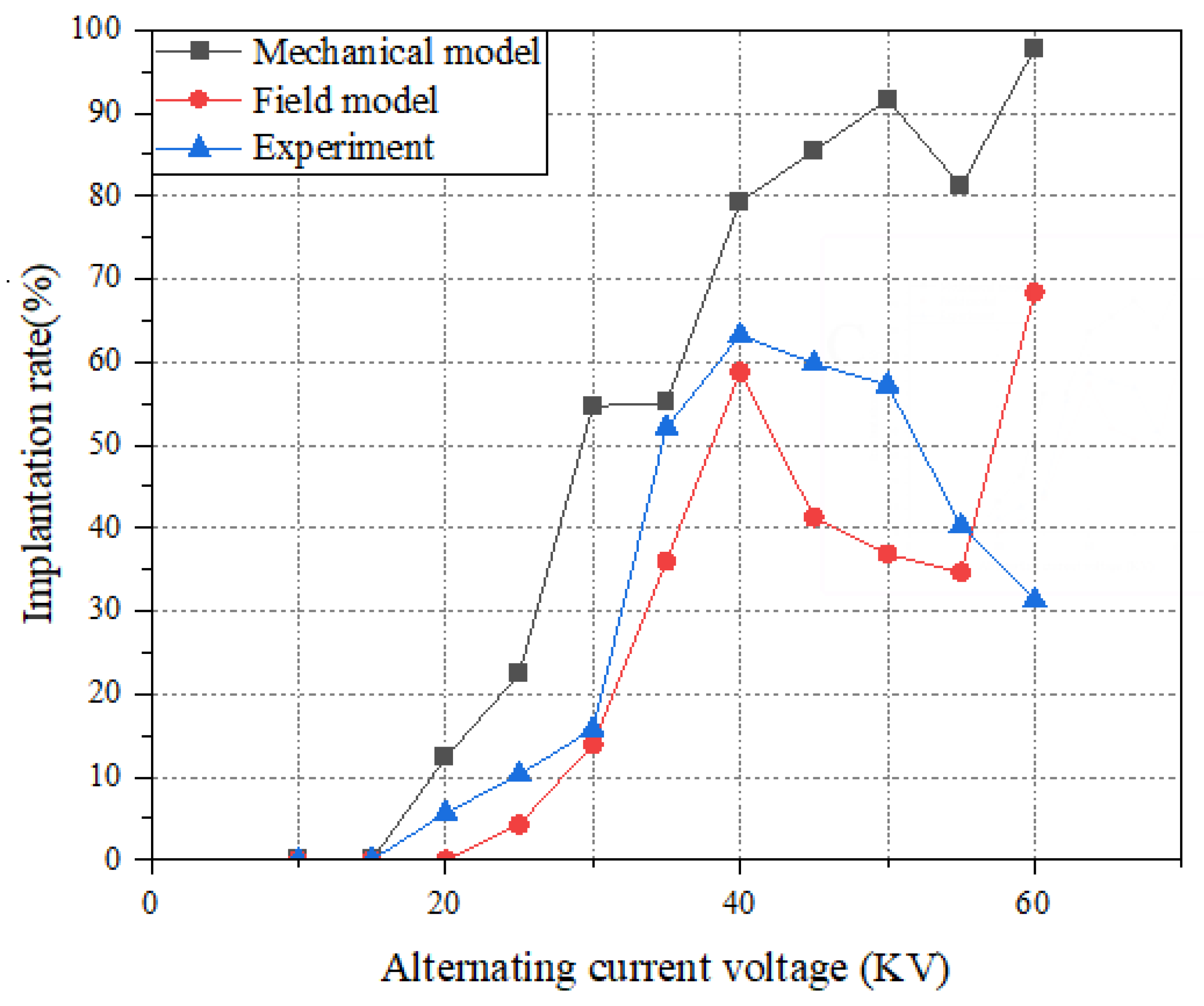
3.2.1. Influence of Pole Plate Voltage
3.2.2. Influence of Pole Plate Spacing
4. Conclusions
Author Contributions
Funding
Institutional Review Board Statement
Informed Consent Statement
Data Availability Statement
Acknowledgments
Conflicts of Interest
References
- Ren, L.; Zhang, G.; Wang, Y.; Zhang, Q.; Wang, F.; Huang, Y. A New In-Process Material Removal Rate Monitoring Approach in Abrasive Belt Grinding. Int. J. Adv. Manuf. Technol. 2019, 104, 2715–2726. [Google Scholar] [CrossRef]
- Zhang, J.; Yang, Y.; Luo, B.; Liu, H.; Li, L. Research on Wear Characteristics of Abrasive Belt and the Effect on Material Removal during Sanding of Medium Density Fiberboard (MDF). Eur. J. Wood Prod. 2021, 79, 1563–1576. [Google Scholar] [CrossRef]
- Leng, Y.F.; Zhang, N. Experiment Research on Abrasive Belt Vibration Grinding Terminal Surface of Work Piece. Adv. Mater. Res. 2011, 154–155, 1240–1243. [Google Scholar] [CrossRef]
- Ren, L.; Wang, N.; Pang, W.; Li, Y.; Zhang, G. Modeling and Monitoring the Material Removal Rate of Abrasive Belt Grinding Based on Vision Measurement and the Gene Expression Programming (GEP) Algorithm. Int. J. Adv. Manuf. Technol. 2022, 120, 385–401. [Google Scholar] [CrossRef]
- Wang, N.; Zhang, G.; Ren, L.; Pang, W.; Li, Y. Novel Monitoring Method for Belt Wear State Based on Machine Vision and Image Processing under Grinding Parameter Variation. Int. J. Adv. Manuf. Technol. 2022, 1–14. [Google Scholar] [CrossRef]
- Chen, F.; Chen, H.; Zhang, L.; Yin, S.; Huang, S.; Zhang, G.; Tang, Q. Controllable Distribution of Ultrafine Diamond Particles by Electrostatic Spray Deposition. Powder Technol. 2019, 345, 267–273. [Google Scholar] [CrossRef]
- Zhao, Y.; Yao, J. Electrostatic Characterization of Electrohydrodynamic Atomization Process for Particle Fabrication. Powder Technol. 2017, 314, 589–598. [Google Scholar] [CrossRef]
- Ohashi, K.; Kawasuji, Y.; Shinji, Y.; Samejima, Y.; Ogawa, S.; Tsukamoto, S. Fundamental Study on Setting of Diamond Abrasive Grains Using Electrostatic Force for Single-Layered Metal Bond Wheel. Adv. Mater. Res. 2012, 565, 40–45. [Google Scholar] [CrossRef]
- Urs, A.; Dragos, C.; Samulia, A.; Iuga, A.; Dascalescu, L. Electrostatic Sizing of Abrasive Particles Using a Free-Fall Corona Separator. Part. Sci. Technol. 2004, 22, 85–92. [Google Scholar] [CrossRef]
- Jeffery, G.B. The Motion of Ellipsoidal Particles Immersed in a Viscous Fluid. Proc. R. Soc. Lond. Ser. A 1922, 102, 161–179. [Google Scholar] [CrossRef] [Green Version]
- Long, Z.; Yao, Q. Evaluation of Various Particle Charging Models for Simulating Particle Dynamics in Electrostatic Precipitators. J. Aerosol. Sci. 2010, 41, 702–718. [Google Scholar] [CrossRef]
- Long, Z.; Yao, Q.; Song, Q.; Li, S. A Second-Order Accurate Finite Volume Method for the Computation of Electrical Conditions inside a Wire-Plate Electrostatic Precipitator on Unstructured Meshes. J. Electrost. 2009, 67, 597–604. [Google Scholar] [CrossRef]
- Lei, H.; Wang, L.Z.; Wu, Z.N. EHD Turbulent Flow and Monte-Carlo Simulation for Particle Charging and Tracing in a Wire-Plate Electrostatic Precipitator. J. Electrost. 2008, 66, 130–141. [Google Scholar] [CrossRef]
- Zhao, L.; Adamiak, K. Numerical Simulation of the Electrohydrodynamic Flow in a Single Wire-Plate Electrostatic Precipitator. IEEE Trans. Ind. Appl. 2008, 44, 683–691. [Google Scholar] [CrossRef]
- Schmid, H.J. On the Modelling of the Particle Dynamics in Electro-Hydrodynamic Flow Fields: II. Influences of Inhomogeneities on Electrostatic Precipitation. Powder Technol. 2003, 135–136, 136–149. [Google Scholar] [CrossRef]
- Yang, Z.; Zheng, C.; Liu, S.; Guo, Y.; Liang, C.; Zhang, X.; Zhang, Y.; Xiang, G. Insights into the Role of Particle Space Charge Effects in Particle Precipitation Processes in Electrostatic Precipitator. Powder Technol. 2018, 339, 606–614. [Google Scholar] [CrossRef]
- Wissdorf, W.; Pohler, L.; Klee, S.; Müller, D.; Benter, T. Simulation of Ion Motion at Atmospheric Pressure: Particle Tracing Versus Electrokinetic Flow. J. Am. Soc. Mass Spectrom. 2012, 23, 397–406. [Google Scholar] [CrossRef] [Green Version]
- Cao, Q.; Li, Z.; Wang, Z.; Han, X. Rotational Motion and Lateral Migration of an Elliptical Magnetic Particle in a Microchannel under a Uniform Magnetic Field. Microfluid. Nanofluid. 2018, 22, 3. [Google Scholar] [CrossRef]
- Gu, Z.; Wei, W. Numerical Modeling Methods for Particle Electrification. In Electrification of Particulates in Industrial and Natural Multiphase Flows; Gu, Z., Wei, W., Eds.; Springer: Singapore, 2017; pp. 117–141. ISBN 978-981-10-3026-0. [Google Scholar]
- White, H.J. Particle Charging in Electrostatic Precipitation. Trans. Am. Inst. Electr. Eng. 1951, 70, 1186–1191. [Google Scholar] [CrossRef]
- Bose, K.; Wood, R.J.K. Optimum Tests Conditions for Attaining Uniform Rolling Abrasion in Ball Cratering Tests on Hard Coatings. Wear 2005, 258, 322–332. [Google Scholar] [CrossRef]


| Field | Force Equations |
|---|---|
| Electric field and fluid field | |
| Colloid layer |
| Parameters | Values | Symbols |
|---|---|---|
| Particle size | 0.035–0.045 [mm] | dp |
| The thickness of the adhesive layer | 0.25 [mm] | d |
| Viscosity coefficient | 4 [GPa·s] | μ1 |
| Particle density (corundum) | 3216 [kg/m3] | |
| Polar plate spacing | 30–100 [mm] | H |
| Alternating current voltage | 0–60 [kV] | |
| Electric field strength | U/H | E |
| Air density | 1.293 [kg/m3] | |
| Air viscosity | 17.9 [μPa·s] | μ2 |
| Particle relative dielectric constant | 6.5 | εr |
| Air dielectric constant | 8.854 × 10⁻¹² F/m | ε0 |
| Materials | Viscosity (MPa·s) | Density (kg/m3) |
|---|---|---|
| Epoxy resin (20 kg) + polyamide (18 kg) + xylene (19 kg) | 150 | 2.0 × 10³ |
| Epoxy resin (20 kg) + polyamide (18 kg) + xylene (18 kg) | 200 | 2.3 × 10³ |
| No. | Voltage/kV | Implantation Rate/% | Relative Error (Mechanical Model)/% | Relative Error (Field Model)/% | ||
|---|---|---|---|---|---|---|
| Mechanical Model | Field Model | Experiment | ||||
| 1 | 10 | 0 | 0 | 0 | 0 | 0 |
| 2 | 15 | 0 | 0 | 0 | 0 | 0 |
| 3 | 20 | 12.3 | 0 | 5.62 | 118.86 | 100 |
| 4 | 25 | 22.38 | 4.26 | 10.28 | 117.70 | 58.56 |
| 5 | 30 | 54.68 | 13.92 | 15.75 | 247.17 | 11.62 |
| 6 | 35 | 55.1 | 36 | 52.11 | 5.74 | 30.92 |
| 7 | 40 | 79.28 | 58.76 | 63.25 | 25.34 | 7.10 |
| 8 | 45 | 85.42 | 41.28 | 59.82 | 42.80 | 30.99 |
| 9 | 50 | 91.62 | 36.88 | 57.21 | 60.15 | 35.54 |
| 10 | 55 | 81.16 | 34.66 | 40.22 | 101.79 | 13.82 |
| 11 | 60 | 97.78 | 68.38 | 31.32 | 212.20 | 118.33 |
| No. | Plate Distance/mm | Implantation Rate/% | Relative Error (Mechanical Model)/% | Relative Error (Field Model)/% | ||
|---|---|---|---|---|---|---|
| Mechanical Model | Field Model | Experiment | ||||
| 1 | 30 | 100 | 100 | 95.42 | 4.80 | 4.80 |
| 2 | 40 | 100 | 100 | 97.57 | 2.49 | 2.49 |
| 3 | 50 | 100 | 68.38 | 93.11 | 7.40 | 26.56 |
| 4 | 60 | 100 | 36.88 | 71.25 | 40.35 | 48.24 |
| 5 | 70 | 100 | 30 | 66.52 | 50.33 | 54.90 |
| 6 | 80 | 99.06 | 26.71 | 35.85 | 176.32 | 25.50 |
| 7 | 90 | 77.86 | 16.48 | 26.51 | 193.70 | 37.83 |
| 8 | 100 | 54.68 | 13.92 | 15.75 | 247.17 | 11.62 |
Publisher’s Note: MDPI stays neutral with regard to jurisdictional claims in published maps and institutional affiliations. |
© 2022 by the authors. Licensee MDPI, Basel, Switzerland. This article is an open access article distributed under the terms and conditions of the Creative Commons Attribution (CC BY) license (https://creativecommons.org/licenses/by/4.0/).
Share and Cite
Zheng, H.; Wang, W.; Gong, L.; Chen, G. Modelling Particle Motion during High-Voltage Electrostatic Abrasive Implantation Based on Multi-Physics Field Coupling. Machines 2022, 10, 406. https://doi.org/10.3390/machines10050406
Zheng H, Wang W, Gong L, Chen G. Modelling Particle Motion during High-Voltage Electrostatic Abrasive Implantation Based on Multi-Physics Field Coupling. Machines. 2022; 10(5):406. https://doi.org/10.3390/machines10050406
Chicago/Turabian StyleZheng, Huifeng, Wenjie Wang, Liang Gong, and Ge Chen. 2022. "Modelling Particle Motion during High-Voltage Electrostatic Abrasive Implantation Based on Multi-Physics Field Coupling" Machines 10, no. 5: 406. https://doi.org/10.3390/machines10050406
APA StyleZheng, H., Wang, W., Gong, L., & Chen, G. (2022). Modelling Particle Motion during High-Voltage Electrostatic Abrasive Implantation Based on Multi-Physics Field Coupling. Machines, 10(5), 406. https://doi.org/10.3390/machines10050406