Article

Parameter Estimation for Robotic Manipulator Systems †

1
Faculty of Science, Engineering and Technology, Swinburne University of Technology, Melbourne, VIC 3122, Australia
2
Discipline of Engineering and Energy Centre for Water, Energy & Waste, Harry Butler Institute, Murdoch University, Perth, WA 6150, Australia
*
Author to whom correspondence should be addressed.
This paper is an extended version of our paper published in Zhu, Q.; Man, Z.; Cao, Z.; Zheng, J.; Wang, H. Parameter Estimation of Robotic Manipulator in Frequency Domain. In Proceedings of the 2021 International Conference on Advanced Mechatronic Systems (ICAMechS), Tokyo, Japan, 9–12 December 2021.
Machines 2022, 10(5), 392; https://doi.org/10.3390/machines10050392
Submission received: 31 March 2022 / Revised: 7 May 2022 / Accepted: 11 May 2022 / Published: 19 May 2022

Abstract

:
In this paper, a novel methodology for estimating the parameters of robotic manipulator systems is proposed. It can be seen that, for the purpose of parameter estimation, the input torque to each joint motor is designed as a linear combination of sinusoids. After the transient responses of joint angles exponentially converge to zero, the steady states of joint angle outputs can be extracted. Since the steady states of joint angles are the equivalent finite Fourier series, the coefficients of the steady state components of joint angles can be further extracted in a fundamental period. With the amazing finding that the steady states contain all dynamic information of manipulator systems, all unknown parameters of the system model can be accurately estimated with the extracted coefficients in finite frequency bands. The simulation results for a two-link manipulator are carried out to illustrate the effectiveness and robustness against measurement noise of the proposed method.

1. Introduction

In modern manufacturing industry, robot manipulator systems are widely adopted in many aspects such as assembling, welding, painting, etc. [1,2,3]. In order to ensure the stability and reliable performance of robot manipulators, many model-based controllers have been proposed [4,5,6,7,8,9,10,11]. The stability of the control performance highly depends on the accuracy of the system dynamic model. To establish the accurate dynamic model, the knowledge of system dynamic parameters is required [12]. However, internal parameter perturbation may occur during long-time continuous operation in many practical applications, which may degrade the reliability of the system operations. Thus, the accurate estimation of system dynamic parameters is of great significance.
Various methodologies have been developed to solve the parameter estimation problem for manipulator systems [13,14,15,16,17,18,19]. One commonly adopted method for identifying the unknown manipulator parameters is the recursive least square method (RLS) [20,21]. The common characteristics of the existing RLS methods are that a cost function needs to be designed; the optimization process will start at a random initial position in the parameter space and proceed along with the surface of that cost function in a series manner [22]. Although many RLS-based approaches have been proposed to complete variable parameter estimation tasks, these methods still have several limitations. For instance, most RLS methods in the time domain have always suffered from low convergence speed [23]; the robustness of the RLS is weak against external disturbances due to its low sensitivity to the new measurements in long-time recursive iteration [24]. Moreover, the local minima problem will happen if the start point has not been selected properly, which may also lead to the degeneration of the estimation performance [25,26].
The Kalman filter (KF) and its variants including extended the Kalman filter (EKF) and unscented the Kalman filter (UKF) have also been proved to be effective of estimating unknown dynamic parameters of manipulator systems [27,28,29,30,31,32]. The KF algorithms employ the stochastic system model, and the model uncertainties and measurement noises are all assumed to be Gaussian. With properly designed KF gains, the posteriori error covariance is minimized, and the optimal estimates of model parameters are obtained in the form of a weighted combination of the priori estimates and measurements. However, the implementation of KF algorithms requires a nominal system model and full system states information [33]. The estimation accuracy will also be degraded due to the unknown distribution of disturbance [34]. In manipulator systems, if the joint angular velocity and angular acceleration are not available, it will be quite hard to formulate the KF algorithm for either estimating system model parameters or system states [35,36]. Furthermore, the robustness of the Kalman filter cannot be guaranteed as well [37,38].
In this paper, a novel parameter estimation scheme is developed for manipulator systems in the frequency domain. To start with, the manipulator system dynamic model has been re-constructed using the linearization technique. It is shown that the information from the other joint can be decoupled and only the joint angular position measurement is required for further parameter estimation. Considering the fact that the transient response of the joint angular position and angular velocity are all damped and will exponentially converge to zero with fast convergence speed, the angular position and angular velocity are dominated by their steady state after sufficient long time. The steady state of angular position can then be extracted from the measurement. In this study, the manipulator system is excited by a linear combination of sinusoidal components. The steady state of the output can also be equivalent to a finite Fourie series. It is shown that, the coefficients of the steady state joint position measurement are all polynomials about the system dynamic parameters and system’s dynamic information has been fully embedded in these coefficients within one fundamental period. Then, the coefficients of the steady state of the angular position can be extracted from the angular position measurement using joint position measurement in one fundamental period. Furthermore, utilizing the relationship among the coefficients of the steady state sinusoidal components of joint position measurement and the system’s dynamic parameters in the frequency domain, all the unknown parameters including the mass of the joint, the length of the joint, etc. can then be estimated based on extracted coefficients.
The advantages of the proposed method can be concluded as: (i) only the steady state part of the measurement in one fundamental period is required to extract the coefficients of the steady state sinusoidal components. (ii) All unknown parameters within the system model can be accurately estimated based on extracted coefficients while the estimation convergence speed is faster than that of traditional recursive estimation schemes and the global optimization mechanism is guaranteed. (iii) The averaging process of extracting the coefficients of steady state sinusoidal components contributes to compensate the effects of the measurement noises. The proposed estimation scheme is robustness against measurements.
Compared to existing parameter estimation approaches, in the proposed method, a nominal model and prior information are not required, only the steady state of the joint position measurement in one fundamental period is needed; the coefficients of the steady state sinusoidal components can all be extracted, based on which all unknown parameters can be estimated in finite frequency bands. In addition, due to the orthogonal properties of the trigonometric base in the sinusoidal components, the computational cost of matrix inversion of the high dimension can be greatly reduced; therefore, the proposed estimation method exhibits high convergence speed, since no recursive process is involved. Moreover, the proposed estimation scheme will show a global optimization mechanism.
The rest of this paper is organized as follows: in Section 2, the dynamic model of a manipulator is reconstructed using a linearization technique. The system’s output response in frequency domain is analyzed. In Section 3, the input torque is designed as a linear combination of sinusoids and the coefficients of steady state sinusoidal components of the measurement are derived and extracted. The unknown parameters are then estimated based on these coefficients. In Section 4, the simulation results are carried out to verify the theoretical analysis and good estimation performance of the proposed method; the robustness of the proposed method is also discussed. In Section 5, the conclusion is briefly summarized.

2. Problem Formulation

Consider a two-link manipulator; the angular position and angular velocity are denoted as q = [ q 1 , q 2 ] T and q ˙ = [ q ˙ 1 , q ˙ 2 ] T , respectively. The dynamic model of this 2 degrees of freedom (DOF) manipulator can be derived as:
D ( q ) q ¨ + C ( q , q ˙ ) q ˙ + G ( q ) = τ  
where τ is the vector of torques applied at two joints and
D ( q ) = [ d 11 d 12 d 21 d 22   ]
{ d 11 = ( m 1 + m 2 ) r 1 2 + m 2 r 2 2 + 2 m 2 r 1 r 2 cos ( q 2 ) + J 1 d 12 = d 21 = m 2 r 2 2 + m 2 r 1 r 2 cos ( q 2 ) d 22 = m 2 r 2 2 + J 2
C ( q , q ˙ ) q ˙ = [ β 12 ( q 2 ) q ˙ 1 2 + 2 β 12 ( q 2 ) q ˙ 1 q ˙ 2 β 12 ( q 2 ) q ˙ 2 2 ]
β 12 ( q 2 ) = m 2 r 1 r 2 sin ( q 2 )
G ( q ) = [ γ 1 ( q 1 , q 2 ) g γ 2 ( q 1 , q 2 ) g ]
γ 1 ( q 1 , q 2 ) = ( ( m 1 + m 2 ) r 1 cos ( q 2 ) + m 2 r 2 cos ( q 1 + q 2 ) )
where m 1 and m 2 are the masses of link 1 and link 2. l 1 and l 2 are the length of link 1 and link 2, respectively. Due to the manufacturing error, the actual values of these dynamic quantities are different from their nominal values. In addition, the parameter perturbation during the operation also degenerates the reliability of the model. Thus, it is of great significance to develop an online parameter estimation scheme to estimate real time values of all robotic mechanical quantities. The system’s model (1) can be further re-written as:
q ¨ = α ( q , q ˙ ) + β ( q ) τ = f ( q , τ )
where
α ( q , q ˙ ) = D 1 ( q ) ( C ( q , q ˙ ) q ˙ G ( q ) )
( q ) = D 1 ( q )
In order to implement the proposed parameter identification algorithm, the Taylor series expansion method has been applied to system (1) for the approximation of a linear system, considering the fact that the manipulator system can be stabilized, and the manipulator joint can remain at an equilibrium position q 0 = [ q 10 , q 20 ] . Meanwhile, the system’s joint angular position and velocity are all assumed to change slowly. Thus, the system can be linearized regarding to the equilibrium position q 0 as:
q ¨ 0 + δ q ¨ = f ( q 0 + δ q , τ 0 + δ τ ) f ( q 0 , τ 0 ) + f q | q 0 , τ 0 δ q + f τ | q 0 , τ 0 δ τ
where q ¨ 0 = f ( q 0 , τ 0 ) ; thus,
δ q ¨ = f q | q 0 , τ 0 δ q + f τ | q 0 , τ 0 δ τ
The linearized system model (12) in the time domain can be further re-expressed in state-space form as:
[ δ q ¨ 1 δ q ¨ 2 ] = [ a 11 a 12 a 21 a 22 ] [ δ q 1 δ q 2 ] + [ b 11 b 12 b 21 b 22 ] [ δ τ 1 δ τ 2 ]
where
{ a 11 = g ( 2 m 1 sin ( q 10 ) ) + m 2 sin ( q 10 ) m 2 sin ( q 10 + 2 q 20 ) l 1 ( 2 m 1 + m 2 m 2 cos ( 2 q 20 ) ) a 12 = g m 2 ( sin ( q 10 + 2 q 20 ) + sin ( q 10 ) ) l 1 ( 2 m 1 + m 2 m 2 cos ( 2 q 20 ) ) a 21 = g ( l 2 m 2 cos 2 ( q 20 ) sin ( q 10 ) l 2 m 2 sin ( q 10 ) l 2 m 1 sin ( q 10 ) + l 1 m 1 cos ( q 10 ) sin ( q 20 ) + l 2 m 2 cos ( q 10 ) cos ( q 20 ) sin ( q 20 ) ) l 1 l 2 ( m 1 + m 2 m 2 cos 2 ( q 20 ) ) a 22 = l 1 2 m 1 + l 1 2 m 2 + 2 l 1 l 2 m 2 cos ( q 20 ) l 1 2 l 2 2 m 2 ( m 1 + m 2 m 2 cos 2 ( q 20 ) )
  { b 11 = 1 l 1 2 ( m 1 + m 2 m 2 cos 2 ( q 20 ) ) b 12 = l 2 + l 1 cos ( q 20 ) l 1 2 l 2 ( m 1 + m 2 m 2 cos 2 ( q 20 ) ) b 21 = b 12 b 22 = l 1 2 m 1 + l 1 2 m 2 + l 2 2 m 2 + 2 l 1 l 2 m 2 cos ( q 20 ) l 1 2 l 2 2 m 2 ( m 1 + m 2 m 2 cos 2 ( q 20 ) )
The transfer functions of system (13) can then be formulated as:
Q 1 ( s ) = b 11 s + a 12 b 21 a 22 b 11 s 2 ( a 11 + a 22 ) s + a 11 a 22 a 12 a 21 U 1 ( s ) + b 12 s + a 12 b 22 a 22 b 12 s 2 ( a 11 + a 22 ) s + a 11 a 22 a 12 a 21 U 2 ( s ) = ( b 11 s + p 1 ) U 1 ( s ) ( s σ 0 ) 2 + ω d 2 + ( b 12 s + p 2 ) U 2 ( s ) [ ( s σ 0 ) 2 + ω d 2 ]
Q 2 ( s ) = b 21 s + a 21 b 11 a 11 b 21 s 2 ( a 11 + a 22 ) s + a 11 a 22 a 12 a 21 U 1 ( s ) + b 22 s + a 21 b 12 a 11 b 22 s 2 ( a 11 + a 22 ) s + a 11 a 22 a 12 a 21 U 2 ( s ) = ( b 21 s + p 3 ) U 1 ( s ) ( s σ 0 ) 2 + ω d 2 + ( b 22 s + p 4 ) U 2 ( s ) [ ( s σ 0 ) 2 + ω d 2 ]
where σ 0 = a 11 + a 22 2 , ω d 2 = ( a 11 a 22 a 12 a 21 ) a 11 + a 22 2 2 = ω 0 2 σ 0 2 . p 1 = a 12 b 21 a 22 b 11 , p 2 = a 12 b 22 a 22 b 12 , p 3 = a 21 b 11 a 11 b 21 , p 4 = a 21 b 12 a 11 b 22 In this case, | σ 0 | is the damping factor, ω 0 is the undamped frequency, and ω d is the damping frequency. In this section, for convenience, it is assumed that:
ω 0 2 σ 0 2 0
In systems (16) and (17), parameters a 11   a 22 , b 11   b 22 are all polynomials with respect to the dynamic quantities. In order to estimate the dynamic quantities of manipulator systems, system parameters need to be obtained first. In the next section, the parameter estimation algorithm is proposed to extract the parameters from the steady state of the joint position output.

3. Main Results

Regarding the system’s transfer function (16) and (17), the input signal has been designed as a linear combination of sinusoidal components as:
u k ( t ) = i = 1 n d k i cos ( ω k i t ) , k = 1 , 2
The corresponding transfer function of the above input signal is given by:
U k ( s ) = i = 1 n d k i s s 2 + ω k i 2 ,   k = 1 , 2
Substituting (20) into (16) and (17) yields:
Q 1 ( s ) = i = 1 n ( ( b 11 s + p 1 ) d 1 i s [ ( s σ 0 ) 2 + ω d 2 ] ( s 2 + ω 1 i 2 ) + ( b 12 s + p 2 ) d 2 i s [ ( s σ 0 ) 2 + ω d 2 ] ( s 2 + ω 2 i 2 ) )  
Q 2 ( s ) = i = 1 n ( ( b 21 s + p 3 ) d 1 i s [ ( s σ 0 ) 2 + ω d 2 ] ( s 2 + ω 1 i 2 ) + ( b 22 s + p 4 ) d 2 i s [ ( s σ 0 ) 2 + ω d 2 ] ( s 2 + ω 2 i 2 ) )

3.1. Estimation of Steady State Coefficients

Using the partial fraction expansion method, the i th component of (21) can be expressed as:
Q 1 i ( s ) = A 11 i ( s σ 0 ) + B 11 i ω d ( s σ 0 ) 2 + ω d 2 + C 11 i s + D 11 i ω 1 i s 2 + ω 1 i 2 + A 12 i ( s σ 0 ) + B 12 i ω d ( s σ 0 ) 2 + ω d 2 + C 12 i s + D 12 i ω 2 i s 2 + ω 2 i 2
Based on (21) and (23), the following relationships can be obtained:
{ A 11 i + C 11 i = 0 A 11 i σ 0 + B 11 i ω d 2 C 11 i σ 0 + D 11 i ω 1 i = d 1 i b 11   A 11 i ω 1 i 2 + C 11 i ω 0 2 2 D 11 i ω i i σ 0 = d 1 i p 1 A 11 i σ 0 ω 11 i 2 + B 11 i ω d ω 11 i 2 + D 11 i ω 11 i ω 0 2 = 0
By solving the equation set (24), A 11 i , B 11 i , C 11 i and D 11 i can be calculated as:
{ A 11 i = 2 ω 11 i σ 0 d 1 i b 11 + d 1 i p 1 ( ω 1 i 2 ω 0 2 ) 4 ω 1 i 2 σ 0 2 + ( ω 1 i 2 ω 0 2 ) 2 B 11 i = ( d 1 i b 21 ) ω d + σ 0 ω d 2 ω 11 i σ 0 d 1 i b 11 d 1 i p 1 ( ω 1 i 2 ω 0 2 ) 4 ω 1 i 2 σ 0 2 + ( ω 1 i 2 ω 0 2 ) 2                           + ω 1 i ω d 2 ω 1 i σ 0 d 1 i p 1 d 1 i b 11 ω 1 i ( ω 1 i 2 ω 0 2 ) 4 ω 1 i 2 σ 0 2 + ( ω 1 i 2 ω 0 2 ) 2 C 11 i = 2 ω 11 i σ 0 d 1 i b 11 d 1 i p 1 ( ω 1 i 2 ω 0 2 ) 4 ω 1 i 2 σ 0 2 + ( ω 1 i 2 ω 0 2 ) 2 D 11 i = 2 ω 1 i σ 0 d 1 i p 1 d 1 i b 11 ω 1 i ( ω 1 i 2 ω 0 2 ) 4 ω 1 i 2 σ 0 2 + ( ω 1 i 2 ω 0 2 ) 2
Similarly, A 21 i , B 21 i , C 21 i and D 21 i can also be obtained as:
{ A 21 i = 2 ω 21 i σ 0 d 2 i b 12 + d 2 i p 2 ( ω 2 i 2 ω 0 2 ) 4 ω 2 i 2 σ 0 2 + ( ω 2 i 2 ω 0 2 ) 2 B 21 i = ( d 2 i b 22 ) ω d + σ 0 ω d 2 ω 21 i σ 0 d 2 i b 12 d 2 i p 2 ( ω 2 i 2 ω 0 2 ) 4 ω 2 i 2 σ 0 2 + ( ω 2 i 2 ω 0 2 ) 2                           + ω 2 i ω d 2 ω 2 i σ 0 d 2 i p 2 d 2 i b 12 ω 2 i ( ω 2 i 2 ω 0 2 ) 4 ω 2 i 2 σ 0 2 + ( ω 2 i 2 ω 0 2 ) 2 C 21 i = 2 ω 21 i σ 0 d 2 i b 12 d 2 i p 2 ( ω 2 i 2 ω 0 2 ) 4 ω 2 i 2 σ 0 2 + ( ω 2 i 2 ω 0 2 ) 2 D 21 i = 2 ω 2 i σ 0 d 2 i p 2 d 2 i b 12 ω 2 i ( ω 2 i 2 ω 0 2 ) 4 ω 2 i 2 σ 0 2 + ( ω 2 i 2 ω 0 2 ) 2
Therefore, the i t h component of the output joint angle (23) can be re-expressed in the time domain as:
q 1 i ( t ) = q 1 t i ( t ) + q 1 s i ( t ) # ( 27 )
where
q 1 t i ( t ) = A 11 i e σ 0 t cos ( ω 1 i t ) + B 11 i e σ 0 t sin ( ω 1 i t ) + A 21 i e σ 0 t c o s ( ω 2 i t ) + B 21 i e σ 0 t s i n ( ω 2 i t )
q 1 i s ( t ) = C 11 i cos ( ω 1 i t ) + D 11 i sin ( ω 1 i t ) + C 12 i c o s ( ω 2 i t ) + D 12 i sin ( ω 2 i t )
where q 1 t i ( t ) is the transient component of the i th term of joint position output while q 1 i s ( t ) is the steady state component. As time t moves towards infinity, with the excitation input signal (19) and the transient response component q 1 t i ( t ) will exponentially decrease to 0 . If the time constant 1 / | σ 0 | is small enough, the joint position output will be dominated by the steady state component. The steady state output can then be formulated as:
q 1 s ( t ) = i = 1 n C 11 i cos ( ω 1 i t ) + D 11 i sin ( ω 1 i t ) + C 12 i c o s ( ω 2 i t ) + D 12 i sin ( ω 2 i t )
To extract the coefficients C 11 i , D 11 i , C 12 i and D 12 i (30) can be expanded into the matrix from as:
q 1 s ( t ) = [ cos ( ω 11 ) , sin ( ω 11 ) , cos ( ω 21 ) , sin ( ω 21 ) , cos ( ω 1 n ) , sin ( ω 1 n ) , cos ( ω 2 n ) , sin ( ω 2 n ) ] [ C 11 D 11 C 2 n D 2 n ]
Taking m samples of each function in (29) gives:
Q 1 = [ q 1 s ( t ( m 1 ) Δ ) , q 1 s ( t ( m 2 ) Δ ) , q 1 s ( t Δ ) , q 1 s ( t ) ] T
where Δ is the sampling period. Substituting (28) into (29) yields:
Q 1   = A 1 P 1 = [ cos ( ω 11 ( t ( m 1 ) Δ ) ) cos ( ω 11 ( t ( m 2 ) Δ ) ) cos ( ω 11 t ) sin ( ω 11 ( t ( m 1 ) Δ ) ) sin ( ω 11 ( t ( m 2 ) Δ ) ) sin ( ω 11 t ) cos ( ω 2 n ( t ( m 1 ) Δ ) ) cos ( ω 2 n ( t ( m 2 ) Δ ) ) cos ( ω 2 n t ) sin ( ω 2 n ( t ( m 1 ) Δ ) ) sin ( ω 2 n ( t ( m 2 ) Δ ) ) sin ( ω 2 n t ) ] [ C 11 D 11 C 2 n D 2 n ]
Using the least square optimization method, the coefficients vector P 1 can be estimated as:
P ^ 1 = ( A 1 T A 1 ) 1 A 1 T Q 1
It is noteworthy that, in the design of the input signal (19), each sinusoidal component satisfies the following orthogonal properties:
0 T cos ( ω k i ) cos ( ω k j ) d t = 0 ,   k = 1 , 2 ,   i j
0 T sin ( ω k i ) sin ( ω k j ) d t = 0 ,   k = 1 , 2 ,   i j
0 T sin ( ω k i ) cos ( ω k j ) d t = 0 ,   k = 1 , 2 ,   i j
In addition,
0 T sin 2 ( ω k i ) d t = T 2 ,   k = 1 , 2
0 T cos 2 ( ω k i ) d t = T 2 ,   k = 1 , 2
In practice, in order to obtain the accurate estimation of the coefficients C 11 i , C 12 i , D 11 i and D 12 i , for i = 1 , 2 , , n , the output measurement needs to be sampled within a fundamental period T . Furthermore, the sampling period Δ is selected to be small enough, (35)–(39) can then be approximated as follows:
0 T cos ( ω k i ) cos ( ω k j ) d t n = 1 m cos ( ω k i ( n 1 ) Δ ) cos ( ω k j ( n 1 ) Δ ) Δ 0 ,   k = 1 , 2 ,   i j
0 T sin ( ω k i ) sin ( ω k j ) d t n = 1 m sin ( ω k i ( n 1 ) Δ ) sin ( ω k j ( n 1 ) Δ ) Δ 0 ,   k = 1 , 2 ,   i j
0 T sin ( ω k i ) cos ( ω k j ) d t n = 1 m sin ( ω k i ( n 1 ) Δ ) cos ( ω k j ( n 1 ) Δ ) Δ 0 ,   k = 1 , 2 ,   i j
0 T sin 2 ( ω k i ) d t n = 1 m sin 2 ( ω k i ( n 1 ) Δ ) Δ T 2 ,   k = 1 , 2
0 T cos 2 ( ω k i ) d t n = 1 m cos 2 ( ω k i ( n 1 ) Δ ) Δ T 2 ,   k = 1 , 2
Based on (40)–(44), the term ( A 1 T A 1 ) 1 in (34) can then be approximate as:
( A 1 T A 1 ) 1 [ T 2 Δ 0 0 0   T 2 Δ ] 1 = 2 Δ T [ 1 0 0 0   1 ]
Furthermore,
A 1 T Q 1 T 2 Δ P 1
Thus,
P ^ 1 = ( A 1 T A 1 ) 1 A 1 T Q 1 2 Δ T A 1 T Q 1 P 1
The steady state coefficients C 11 i , D 11 i , C 12 i and D 12 i . can then be numerically estimated according to (47) as:
{ C ^ 11 i = 2 T k = 1 m q 1 s ( t ( k 1 ) Δ ) cos ( ω 1 i ( t ( k 1 ) Δ ) ) Δ D ^ 11 i = 2 T k = 1 m q 1 s ( t ( k 1 ) Δ ) sin ( ω 1 i ( t ( k 1 ) Δ ) ) Δ C ^ 12 i = 2 T k = 1 m q 1 s ( t ( k 1 ) Δ ) cos ( ω 2 i ( t ( k 1 ) Δ ) ) Δ D ^ 12 i = 2 T k = 1 m q 1 s ( t ( k 1 ) Δ ) sin ( ω 2 i ( t ( k 1 ) Δ ) ) Δ
It is shown from (45) that the computational cost of the matrix inverse calculation has been greatly decreased after the numerical approximation of the sinusoidal components based on their orthogonal properties. Moreover, the averaging process in (48) also contributes to reduce the effects of the measurement noises and, as a result, guarantee the robustness of the proposed algorithm against measurement noises.
Since the accurate estimation of the coefficient vector P 1   of the steady state of the joint position measurement can be obtained from (48), the identification algorithm for estimating the unknown dynamic parameters can be further developed.

3.2. Estimation of Unknown Dynamic Parameters

As discussed in (27)–(30), the joint angular position output is dominated by its steady state components after sufficient long time; thus:
q 1 i ( t ) q 1 s i ( t ) = C 11 i cos ( ω 1 i t ) + D 11 i sin ( ω 1 i t ) + C 12 i c o s ( ω 2 i t ) + D 12 i sin ( ω 2 i t )
Based on (21) and (23), the following relations can be derived:
C 11 i ω 1 i 2 = C 11 i ω 0 2 2 D 11 i ω 1 i σ 0 d 1 i P 1
D 1 i ω 1 i 2 = D 1 i ω 0 2 + 2 C 1 i ω 1 i σ 0 + d 1 i ω 1 i b 11
Since C 11 i and D 11 i can be accurately estimated via (45), (50) and (51) can then be re-written as:
C ^ 11 i ω 1 i 2 = C ^ 11 i ω ^ 0 2 2 D ^ 11 i ω 1 i σ ^ 0 d 1 i P ^ 1
D ^ 11 i ω 1 i 2 = D ^ 11 i ω ^ 0 2 + 2 C ^ 11 i ω 1 i σ ^ 0 + d 1 i ω 1 i b ^ 11
To estimate unknown parameters, sufficient number of coefficients C 11 and D 11 need to be obtained via (47). Then, the following data equation in matrix form can be derived:
Q 2 = A 2 P 2
where
Q 2 = [ C ^ 111 ω 11 2 C ^ 112 ω 12 2 D ^ 111 ω 11 2 C ^ 11 n ω 1 n 2 ] T
A 2 = [ C ^ 111 C ^ 112 D ^ 111 D ^ 11 n 2 D ^ 112 ω 12 2 D ^ 112 ω 12 2 C ^ 111 ω 11 2 C ^ 11 n ω 1 n d 11 d 12 0 0 0 0 d 11 ω 11 d 1 n ω 1 n ]
P 2 = [ ω ^ 0 2 σ ^ 0 P ^ 1 b ^ 11 ] T
Using the least square method, the parameter vector P 2 can be estimated as:
P 2 = ( A 2 T A 2 ) 1 A 2 T Q 2
where all elements in P 2 are equations with respect to the manipulator’s mechanical quantities including the mass of the link, the length of the link, etc.
Similarly, the i th component of (22) can also be expanded using the partial fraction expansion method as:
Q 2 i ( s ) = A 21 i ( s σ 0 ) + B 21 i ω d ( s σ 0 ) 2 + ω d 2 + C 21 i s + D 21 i ω 1 i s 2 + ω 1 i 2 + A 22 i ( s σ 0 ) + B 22 i ω d ( s σ 0 ) 2 + ω d 2 + C 22 i s + D 22 i ω 2 i s 2 + ω 2 i 2
Applying the same process, m samples of the second joint’s angular position measurement are sampled within one fundamental period; sample period Δ is selected to be sufficiently small. The coefficients of the steady state component of (59) can be numerically estimated as:
{ C ^ 21 i = 2 T k = 1 m q 2 s ( t ( k 1 ) Δ ) cos ( ω 1 i ( t ( k 1 ) Δ ) ) Δ   D ^ 21 i = 2 T k = 1 m q 2 s ( t ( k 1 ) Δ ) sin ( ω 1 i ( t ( k 1 ) Δ ) ) Δ C ^ 22 i = 2 T k = 1 m q 2 s ( t ( k 1 ) Δ ) cos ( ω 2 i ( t ( k 1 ) Δ ) ) Δ D ^ 22 i = 2 T k = 1 m q 2 s ( t ( k 1 ) Δ ) sin ( ω 2 i ( t ( k 1 ) Δ ) ) Δ
Based on (22) and (59), the following relationships can be obtained:
C 21 i ω 2 i 2 = C 21 i ω 0 2 2 D 21 i ω 2 i σ 0 d 2 i P 3
D 2 i ω 2 i 2 = D 2 i ω 0 2 + 2 C 2 i ω 2 i σ 0 + d 2 i ω 2 i b 21
Since C 21 i and D 21 i can be accurately estimated via (50), (51) and (60) can then be re-written as:
C ^ 21 i ω 2 i 2 = C ^ 21 i ω ^ 0 2 2 D ^ 21 i ω 2 i σ ^ 0 d 2 i P ^ 3
D ^ 21 i ω 2 i 2 = D ^ 21 i ω ^ 0 2 + 2 C ^ 21 i ω 2 i σ ^ 0 + d 2 i ω 1 i b ^ 21
To estimate unknown parameters, a sufficient number of coefficients C 21 and D 21 needs to be obtained via (60). Then, the following data equation in matrix form can be derived:
Q 3 = A 3 P 3
where
Q 3 = [ C ^ 211 ω 21 2 C ^ 212 ω 22 2 D ^ 211 ω 21 2 C ^ 21 n ω 2 n 2 ] T
A 3 = [ C ^ 211 C ^ 212 D ^ 211 D ^ 21 n 2 D ^ 212 ω 22 2 D ^ 212 ω 22 2 C ^ 211 ω 21 2 C ^ 21 n ω 2 n d 21 d 22 0 0 0 0 d 21 ω 21 d 2 n ω 2 n ]
P 3 = [ ω ^ 0 2 σ ^ 0 p ^ 3 b ^ 21 ] T
Using the least square method, the parameter vector P 3 can be estimated as:
P 3 = ( A 3 T A 3 ) 1 A 3 T Q 3
Once P 2 and P 3 can be estimated via (58) and (69), respectively, all the unknown system dynamic parameters as well as the dynamic quantities can then be derived.
In the proposed method, the parameter estimator for each joint is separately designed. Since the dynamic information is embedded within the steady state of the joint angle measurement, only the joint angle measurement in one fundamental period is required to estimate all dynamic parameters. Meanwhile, the orthogonality of the trigonometric base function contributes to reducing the computation load of the high dimension matrix. As a result, the proposed method can be extended to high DOF manipulators.

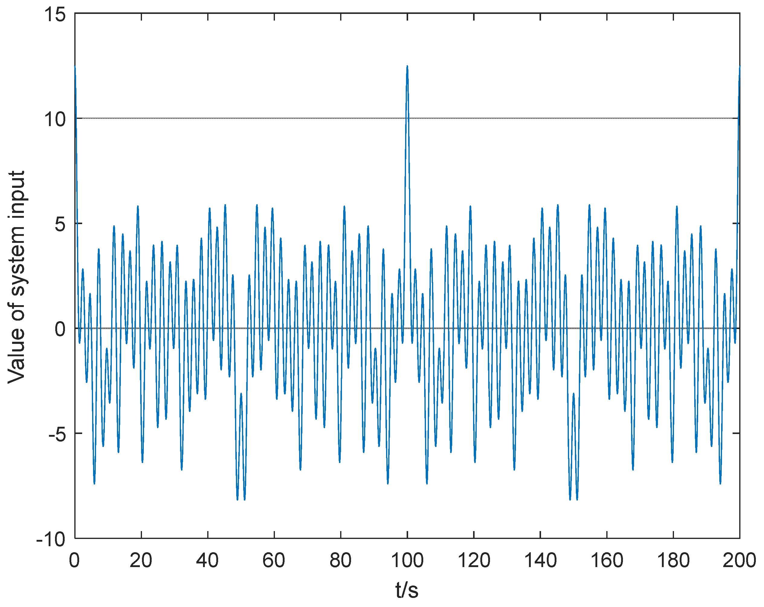
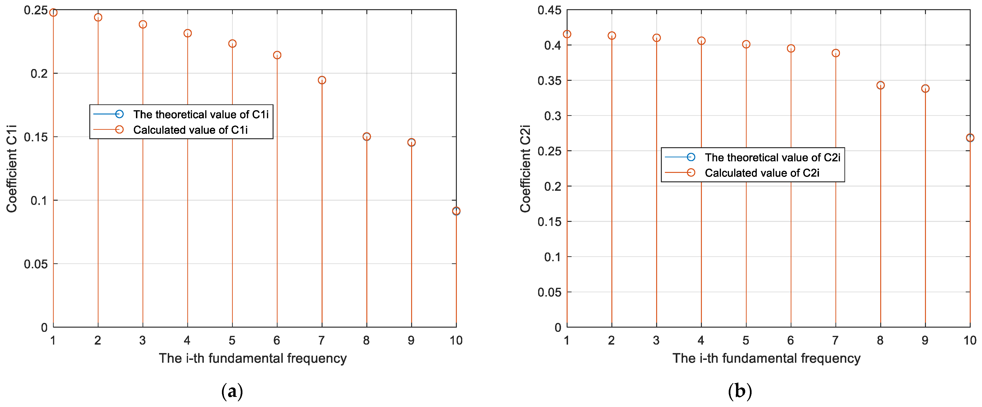
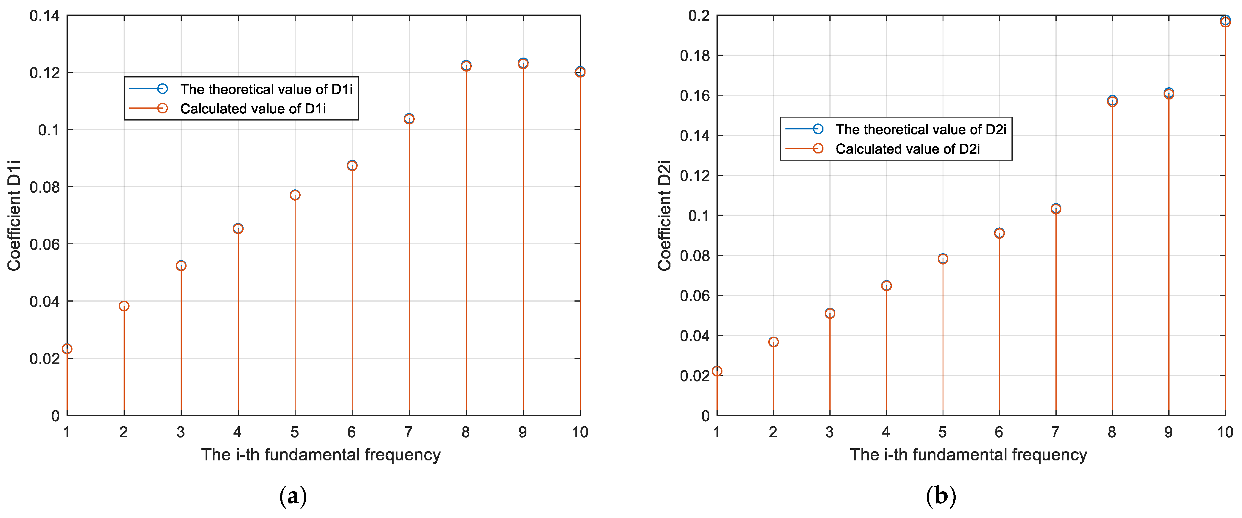
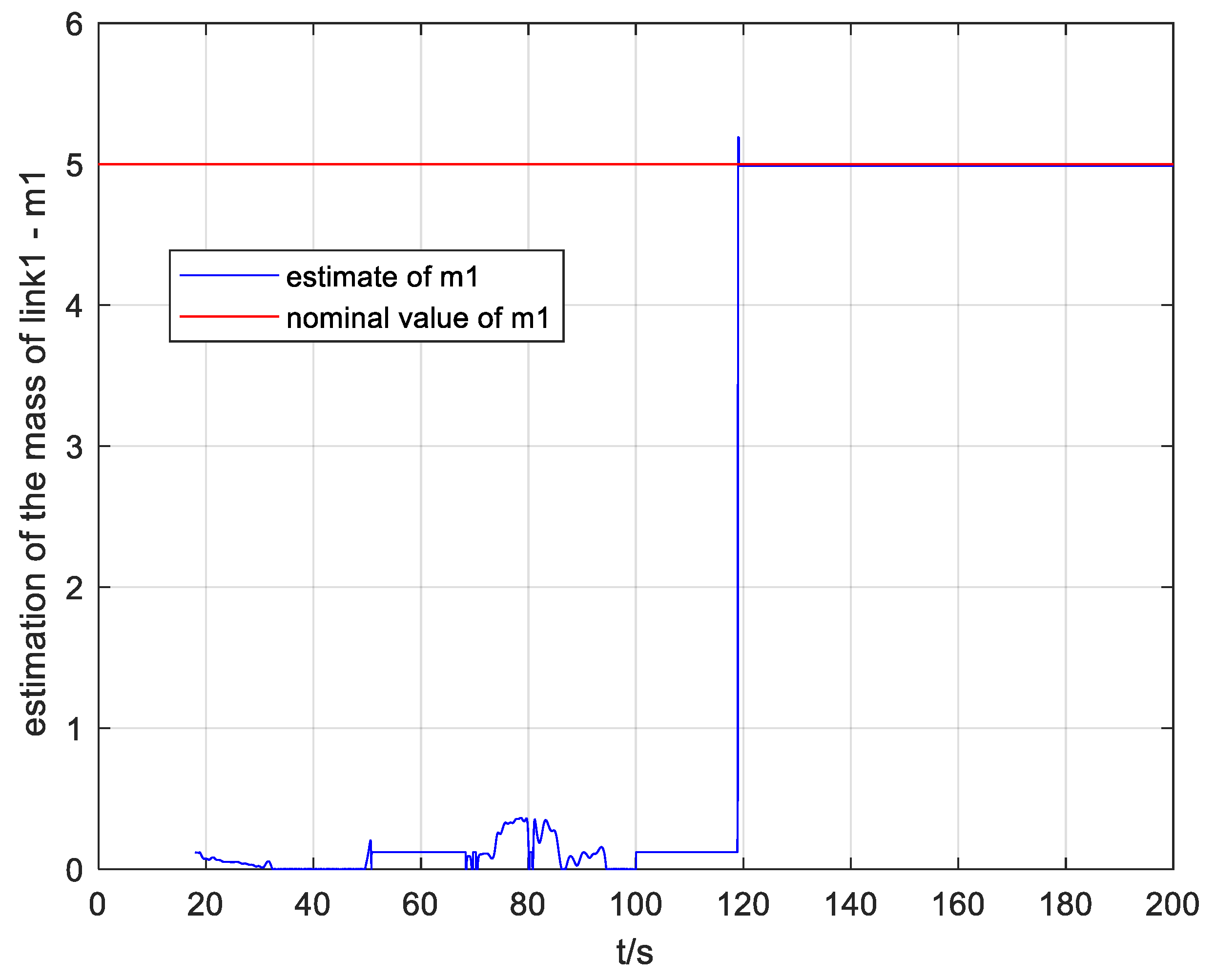
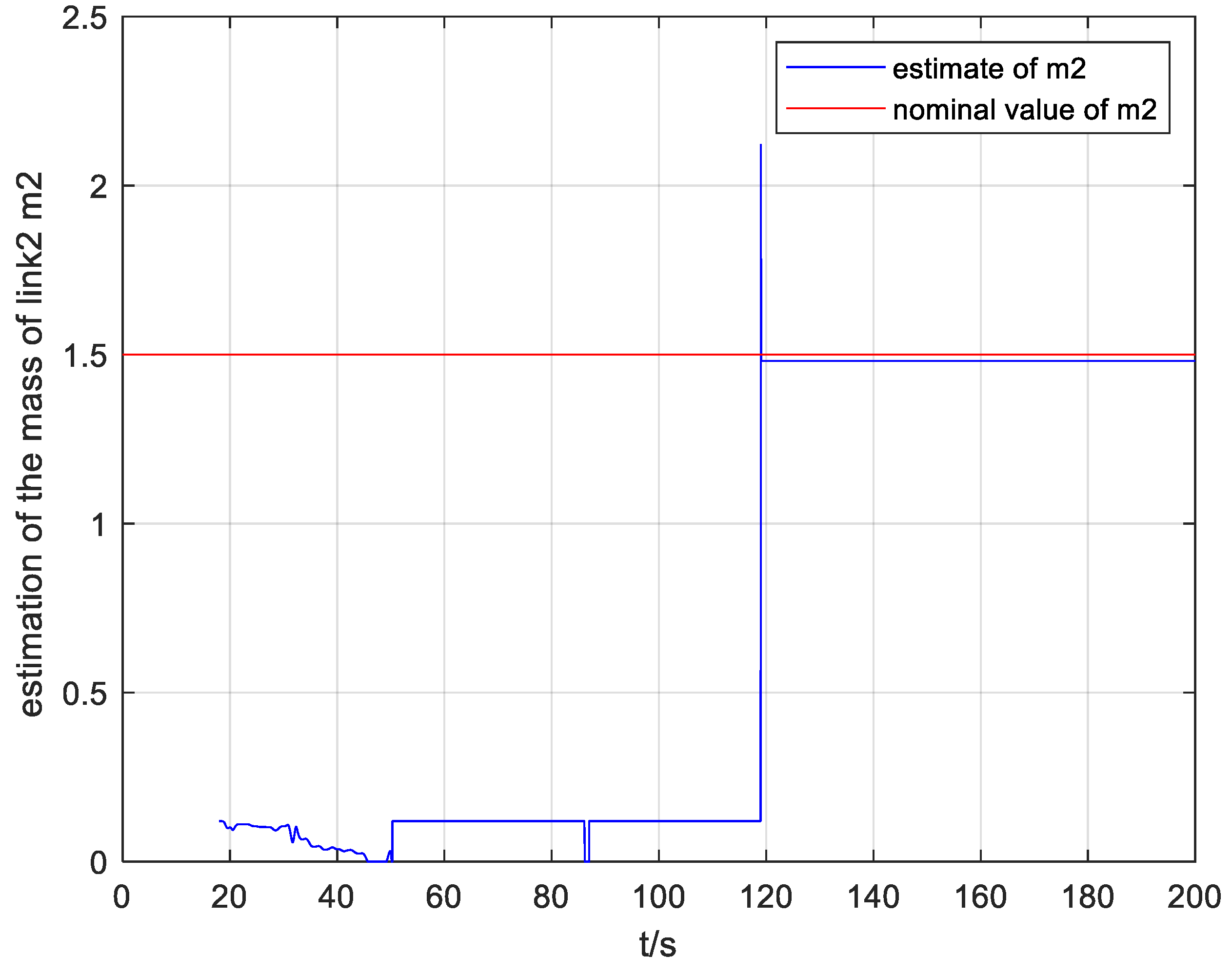
4. Simulation Results

In this section, simulation with a 2-DOF manipulator is performed to verify the feasibility of the proposed parameter estimation algorithm. The nominal values of robotic manipulator parameters are given in the Table 1 [39]:
In this study, the masses of two links are supposed to be unknown. The input torque is designed to be a linear combination of 10 sinusoidal components as shown in Table 2 [39]. The fundamental frequency is selected to be f 0 = 0.01   Hz and ω 0 = 2 π f 0 .
The system input torque with 10 sinusoidal components is shown in Figure 1 [39]. The above torque has been applied to both joints at the same time.
The comparison between the theoretical value and calculated value of coefficients C 11   C 21 , D 11 and D 21 is illustrated in Figure 2 and Figure 3 [39], respectively:
It can be seen from Figure 2 and Figure 3 that, with the fundamental frequency f 0 = 0.01   Hz as the sampling interval and 10 consecutive components, the coefficients of the steady state components of the joint angular position can be accurately estimated based on (48) and (60).
In practical implementations, the measurement of the angular position is vulnerable to being affected by the sensor noise. In order to illustrate the robustness of the proposed identification algorithm against the measurement noises, a white noise d = 0.1 r a n d ( ) is manually added to system output to simulate the actual measurement. The estimation performance of two unknown link masses can be seen in Figure 4 and Figure 5 [39], respectively.
It can be seen from Figure 4 and Figure 5 that the unknown parameters derived based on (58) and (65) can well approximate their actual values. The effect of measurement noises has been reasonably compensated by the averaging process during the calculation of the steady state coefficients in (48) and (60).
To illustrate the accuracy of the estimation, the RMSEs (root-mean square error) for two joints are calculated:
r m s e m 1   = 1.0568
r m s e m 2   = 1.5420

5. Conclusions

In this paper, a novel mythology to estimate the unknown parameters of the robotic manipulator system in frequency domain has been proposed. It is seen that the joint angular position measurement will be dominated by its steady state component after sufficient long time. By designing the input signal to be a linear combination of sinusoidal components, the steady state component of the measurement is equivalent to a finite Fourie series. It is shown that all system dynamic information is embedded in the coefficients of the steady state component within one fundamental period. Thus, the coefficients of the steady state sinusoidal component of the joint angular position output are first extracted. By utilizing the relationship among these coefficients and the system’s dynamic parameters in the frequency domain, all unknown dynamic parameters and mechanical quantities can be estimated accurately. It is expected that this new kind of new estimation scheme can be widely applied in various industrial applications where the systems suffer from uncertainties and disturbances.

Author Contributions

Conceptualization, Q.Z.; methodology, Q.Z.; software, Z.M.; validation, Z.C.; formal analysis, Z.M.; investigation, Z.C.; resources, J.Z.; data curation, Z.M.; writing—original draft preparation, Q.Z.; writing—review and editing, Z.M.; visualization, Z.C.; supervision, H.W.; project administration, H.W. All authors have read and agreed to the published version of the manuscript.

Funding

This research received no external funding.

Institutional Review Board Statement

Not applicable.

Informed Consent Statement

Not applicable.

Data Availability Statement

Data sharing not applicable.

Acknowledgments

The first author received financial support from the Chinese Scholarship Council (No. 201808330398).

Conflicts of Interest

The authors declare no conflict of interest.

References

  1. Tereshchuk, V.; Stewart, J.; Bykov, N.; Pedigo, S.; Devasia, S.; Banerjee, A.G. An efficient scheduling algorithm for multi-robot task allocation in assembling aircraft structures. IEEE Robot. Autom. Lett. 2019, 4, 3844–3851. [Google Scholar] [CrossRef] [Green Version]
  2. Asadi, E.; Li, B.; Chen, I.M. Pictobot: A cooperative painting robot for interior finishing of industrial developments. IEEE Robot. Autom. Mag. 2018, 25, 82–94. [Google Scholar] [CrossRef]
  3. Wang, X.; Shi, Y.; Ding, D.; Gu, X. Double global optimum genetic algorithm–particle swarm optimization-based welding robot path planning. Eng. Optim. 2016, 48, 299–316. [Google Scholar] [CrossRef]
  4. Zhihong, M.; Paplinski, A.P.; Wu, H.R. A robust MIMO terminal sliding mode control scheme for rigid robotic manipulators. IEEE Trans. Autom. Control. 1994, 39, 2464–2469. [Google Scholar] [CrossRef]
  5. Yu, X.; Man, Z. Terminal sliding mode observers for a class of nonlinear systems. Automatica 2010, 46, 1401–1404. [Google Scholar]
  6. Atkeson, C.G.; An, C.H.; Hollerbach, J.M. Estimation of inertial parameters of manipulator loads and links. Int. J. Robot. Res. 1986, 5, 101–119. [Google Scholar] [CrossRef]
  7. Yu, S.; Yu, X.; Shirinzadeh, B.; Man, Z. Continuous finite-time control for robotic manipulators with terminal sliding mode. Automatica 2005, 41, 1957–1964. [Google Scholar] [CrossRef]
  8. Feng, Y.; Yu, X.; Man, Z. Non-singular terminal sliding mode control of rigid manipulators. Automatica 2002, 38, 2159–2167. [Google Scholar] [CrossRef]
  9. Nubert, J.; Köhler, J.; Berenz, V.; Allgöwer, F.; Trimpe, S. Safe and fast tracking on a robot manipulator: Robust mpc and neural network control. IEEE Robot. Autom. Lett. 2020, 5, 3050–3057. [Google Scholar] [CrossRef] [Green Version]
  10. Ali, K.; Ullah, S.; Mehmood, A.; Mostafa, H.; Marey, M.; Iqbal, J. Adaptive FIT-SMC Approach for an Anthropomorphic Manipulator with Robust Exact Differentiator and Neural Network-Based Friction Compensation. IEEE Access 2022, 10, 3378–3389. [Google Scholar] [CrossRef]
  11. Ullah, S.; Khan, Q.; Mehmood, A.; Kirmani, S.A.M.; Mechali, O. Neuro-adaptive fast integral terminal sliding mode control design with variable gain robust exact differentiator for under-actuated quadcopter UAV. ISA Trans. 2022, 120, 293–304. [Google Scholar] [CrossRef] [PubMed]
  12. Thomas, M.J.; George, S.; Sreedharan, D.; Joy, M.; Sudheer, A. Dynamic modeling, system identification and comparative study of various control strategies for a spatial parallel manipulator. Proceedings of the Institution of Mechanical Engineers, Part I. J. Syst. Control. Eng. 2022, 236, 270–293. [Google Scholar]
  13. Danesh, M.; Sheikholeslam, F.; Keshmiri, M. An adaptive manipulator controller based on force and parameter estimation. IEICE Transactions on Fundamentals of Electronics. Commun. Comput. Sci. 2006, 89, 2803–2811. [Google Scholar]
  14. Yang, C.; Jiang, Y.; He, W.; Na, J.; Li, Z.; Xu, B. Adaptive parameter estimation and control design for robot manipulators with finite-time convergence. IEEE Trans. Ind. Electron. 2018, 65, 8112–8123. [Google Scholar] [CrossRef]
  15. Na, J.; Mahyuddin, M.N.; Herrmann, G.; Ren, X.; Barber, P. Robust adaptive finite-time parameter estimation and control for robotic systems. Int. J. Robust Nonlinear Control 2015, 25, 3045–3071. [Google Scholar] [CrossRef] [Green Version]
  16. Mohanty, A.; Yao, B. Indirect adaptive robust control of hydraulic manipulators with accurate parameter estimates. IEEE Trans. Control. Syst. Technol. 2010, 19, 567–575. [Google Scholar] [CrossRef]
  17. Gautier, M.; Janot, A.; Vandanjon, P.O. A new closed-loop output error method for parameter identification of robot dynamics. IEEE Trans. Control. Syst. Technol. 2012, 21, 428–444. [Google Scholar] [CrossRef] [Green Version]
  18. Liu, S.-P.; Ma, Z.-Y.; Chen, J.-L.; Cao, J.-F.; Fu, Y.; Li, S.-Q. An improved parameter identification method of redundant manipulator. Int. J. Adv. Robot. Syst. 2021, 18, 17298814211002118. [Google Scholar] [CrossRef]
  19. Guo, Q.; Chen, Z.; Shi, Y.; Liu, G. Model identification and parametric adaptive control of hydraulic manipulator with neighborhood field optimization. IET Control. Theory Appl. 2021, 15, 1599–1614. [Google Scholar] [CrossRef]
  20. De Souza, D.A.; Batista, J.G.; Vasconcelos, F.J.S.; Dos Reis, L.L.N.; Machado, G.F.; Costa, J.R.; Junior, J.N.N.; Silva, J.L.N.; Rios, C.S.N.; Junior, A.B.S. Identification by Recursive Least Squares With Kalman Filter (RLS-KF) Applied to a Robotic Manipulator. IEEE Access 2021, 9, 63779–63789. [Google Scholar] [CrossRef]
  21. Batista, J.; Souza, D.; Dos Reis, L.; Barbosa, A.; Araújo, R. Dynamic model and inverse kinematic identification of a 3-DOF manipulator using RLSPSO. Sensors 2020, 20, 416. [Google Scholar] [CrossRef] [PubMed] [Green Version]
  22. Wu, J.; Wang, J.; You, Z. An overview of dynamic parameter identification of robots. Robot. Comput. Integr. Manuf. 2010, 26, 414–419. [Google Scholar]
  23. Pradhan, S.K.; Subudhi, B. Position control of a flexible manipulator using a new nonlinear self-tuning PID controller. IEEE/CAA J. Autom. Sin. 2018, 7, 136–149. [Google Scholar] [CrossRef]
  24. Shang, W.; Cong, S.; Kong, F. Identification of dynamic and friction parameters of a parallel manipulator with actuation redundancy. Mechatronics 2010, 20, 192–200. [Google Scholar] [CrossRef]
  25. Urrea, C.; Pascal, J. Parameter identification methods for real redundant manipulators. J. Appl. Res. Technol. 2017, 15, 320–331. [Google Scholar] [CrossRef]
  26. Jia, J.; Zhang, M.; Zang, X.; Zhang, H.; Zhao, J. Dynamic parameter identification for a manipulator with joint torque sensors based on an improved experimental design. Sensors 2019, 19, 2248. [Google Scholar] [CrossRef] [PubMed] [Green Version]
  27. Klimchik, A.; Furet, B.; Caro, S.; Pashkevich, A. Identification of the manipulator stiffness model parameters in industrial environment. Mech. Mach. Theory 2015, 90, 1–22. [Google Scholar] [CrossRef] [Green Version]
  28. Du, G.; Zhang, P. Online serial manipulator calibration based on multisensory process via extended Kalman and particle filters. IEEE Trans. Ind. Electron. 2014, 61, 6852–6859. [Google Scholar]
  29. Partovibakhsh, M.; Liu, G. An adaptive unscented Kalman filtering approach for online estimation of model parameters and state-of-charge of lithium-ion batteries for autonomous mobile robots. IEEE Trans. Control. Syst. Technol. 2014, 23, 357–363. [Google Scholar] [CrossRef]
  30. Castañeda, C.E.; Esquivel, P. Decentralized neural identifier and control for nonlinear systems based on extended Kalman filter. Neural Netw. 2012, 31, 81–87. [Google Scholar] [CrossRef]
  31. Nguyen, H.N.; Zhou, J.; Kang, H.J. A calibration method for enhancing robot accuracy through integration of an extended Kalman filter algorithm and an artificial neural network. Neurocomputing 2015, 151, 996–1005. [Google Scholar] [CrossRef]
  32. Song, S.; Dai, X.; Huang, Z.; Gong, D. Load parameter identification for parallel robot manipulator based on extended Kalman filter. Complexity 2020, 2020, 8816374. [Google Scholar] [CrossRef]
  33. Cantelli, L.; Muscato, G.; Nunnari, M.; Spina, D. A joint-angle estimation method for industrial manipulators using inertial sensors. IEEE/ASME Trans. Mechatron. 2015, 20, 2486–2495. [Google Scholar] [CrossRef]
  34. Nguyen, H.-N.; Zhou, J.; Kang, H.-J.; Ro, Y.-S. Robot Geometric Parameter Identification with Extended Kalman Filtering Algorithm. International Conference on Intelligent Computing; Springer: Berlin/Heidelberg, Germany, 2013; pp. 165–170. [Google Scholar]
  35. Jiang, Z.; Zhou, W.; Li, H.; Mo, Y.; Ni, W.; Huang, Q. A new kind of accurate calibration method for robotic kinematic parameters based on the extended Kalman and particle filter algorithm. IEEE Trans. Ind. Electron. 2017, 65, 3337–3345. [Google Scholar] [CrossRef]
  36. Zhong, X.; Zhong, X.; Peng, X. Robust Kalman filtering cooperated Elman neural network learning for vision-sensing-based robotic manipulation with global stability. Sensors 2013, 13, 13464–13486. [Google Scholar] [CrossRef] [Green Version]
  37. Urrea, C.; Pascal, J. Design, simulation, comparison and evaluation of parameter identification methods for an industrial robot. Comput. Electr. Eng. 2018, 67, 791–806. [Google Scholar] [CrossRef]
  38. Muradore, R.; Fiorini, P. A PLS-based statistical approach for fault detection and isolation of robotic manipulators. IEEE Trans. Ind. Electron. 2011, 59, 3167–3175. [Google Scholar] [CrossRef]
  39. Zhu, Q.; Man, Z.; Cao, Z.; Zheng, J.; Wang, H. Parameter Estimation of Robotic Manipulator in Frequency Domain. In Proceedings of the 2021 International Conference on Advanced Mechatronic Systems (ICAMechS), Tokyo, Japan, 9–12 December 2021. [Google Scholar]
Figure 1. Input torque signal τ .
Machines 10 00392 g001
Figure 2. (a) The theoretical value and calculated value of C 11 i ; (b) the theoretical value and calculated value of C 21 i .
Machines 10 00392 g002
Figure 3. (a) The theoretical value and calculated value of D 11 i ; (b) the theoretical value and calculated value of D 21 i .
Machines 10 00392 g003
Figure 4. Estimation of link 1′s mass m 1 .
Machines 10 00392 g004
Figure 5. Estimation of link 2′s mass m 2 .
Machines 10 00392 g005
Table 1. Parameter of the robotic manipulator.
ParametersValues
Mass   of   link   1   m 1   ( kg ) 5
Mass   of   link   2   m 2   ( kg ) 1.5
Inertial   of   link   1   j 1   ( kg   · m 2 ) 5
Inertial   of   link   2   j 2   ( kg   · m 2 ) 5
Length   of   link   1   l 1   ( m ) 1
Length   of   link   2   l 2   ( m ) 0.8
Table 2. Sinusoidal components of the input torque signal τ 1 .
i th ComponentFrequencyAmplitude
1 3 ω 0 0.2
2 5 ω 0 1.5
3 7 ω 0 0.3
4 9 ω 0 0.5
5 11 ω 0 0.7
6 13 ω 0 0.8
7 17 ω 0 1.0
8 21 ω 0 1.2
9 27 ω 0 1.4
10 42 ω 0 2.0
Publisher’s Note: MDPI stays neutral with regard to jurisdictional claims in published maps and institutional affiliations.

