Stiffness-Oriented Placement Optimization of Machining Robots for Large Component Flexible Manufacturing System

Abstract

A large component flexible manufacturing system provides more application scenarios for industrial robots, and, in turn, these robots exhibit competitive advantages in machining applications. However, the structural characteristic of low stiffness is the main obstacle for the industrial robot. Aiming at obtaining sufficient stiffness in the whole machining process, this paper focuses on robot placement optimization in the flexible manufacturing of large components. The geometric center of the machined feature is selected as, firstly, the base point, and the center-reachable placement space of the robot base is obtained by establishing the kinematic model considering a variety of motion constraints. Then, according to the reachability of the machining feature contour, the global placement space meeting all machining boundaries is further extracted. The mapping relationship between joint force and posture is established, and the most suitable robot placement is selected based on the criterion of global stiffness optimization. A series of numerical and finite element simulations verify the correctness and effectiveness of the proposed optimization strategy. The developed stiffness-oriented placement planning algorithm can provide beneficial references for robotic machining applications.

1. Introduction

In general, traditional computer numerical control (CNC) machine tools in the field of mechanical manufacturing are dedicated to high-accuracy tasks, such as milling, grinding, and drilling, while industrial robots are usually adopted for dull and dirty work scenes to replace human workers. The robots are mainly designed to perform repetitive work with relatively low accuracy, such as transferring, palletizing, and painting [1,2,3]. However, owing to their considerable advantages such as high flexibility, large workspace, and cost-efficiency, industrial robots have attracted increasing attention in the manufacturing industry. With tremendous support from the academic and industrial communities, robots have become viable and competitive candidates in machining applications, especially for large-scale components [4,5] which usually exceeds 10 m in size, far beyond the processing range of conventional CNC technology. Moreover, large-scale components are usually produced in a single part or small batch. Hence, the flexible machining system based on industrial robot has also been proposed [6,7,8,9].

Unfortunately, low stiffness is the main obstacle for industrial machining robots. The stiffness of robots is generally less than 1 $\mathrm{N}/\mathsf{\mu }\mathrm{m}$, which is only one-fiftieth of CNC machine tools [10,11]. Due to low stiffness, the end-effector of the machining robot suffers from static deformation and dynamic vibration in machining applications, and large deformation can seriously deteriorate manufacturing accuracy, which results in poor processing quality. Although the active control method can be used to improve machining accuracy [12,13,14], it undoubtedly increases the complexity of the robotic system in the machining field. Hence, exhausting the robot’s potential to achieve the optimal stiffness design has become a hot issue in recent robotics research. Simultaneously, the initial placement of the workpiece with respect to the machining robot directly affects the robot configuration and stiffness along the processing path [15,16]. Therefore, it is of great significance to consider the stiffness of the robot in order to achieve the optimal placement of the machining robot.

The industrial robot’s stiffness is an important index to measure machining performance, and stiffness is directly related to robot posture. In recent decades, many researchers have discussed robot stiffness design and optimization in machining scenes [17,18,19]. Salisbury [20] proposed a general stiffness model of the mobile robot. On this basis, many researchers have proposed methods of stiffness design and stiffness identification in order to further investigate the stiffness properties of machining robots. Combined with the real industrial environment, Klimchik et al. [21] established the stiffness identification model of the mobile manipulator, and the result better simulated real working conditions owing to a consideration of the effect of elastic force. Bu et al. [22] adopted the Cartesian compliance model to depict drilling robot stiffness, and established the relationship between the robot stiffness characteristic and machining quality. In order to predict the deformation of the end-effector under the machining force, similarly, Celikag et al. [23] presented the Cartesian stiffness optimization method for serial robots, and the result effectively improved the stiffness and avoided chatter for the milling tasks. Considering the deformation for robotic machining tasks, Lin et al. [24] focused on the spindle configuration strategy affecting the accuracy of the end-effector, and the experimental results validated the effectiveness of the proposed optimized spindle configuration model. Based on mapping between the milling force and deformation, Chen et al. [25] optimized robot posture and feed orientation of the end-effector to obtain higher contour machining accuracy.

For robotic machining applications, the relative position of robot and workpiece is crucial for accuracy and efficiency, and the issue of how to optimize the base position is still under heated discussion. Based on the established approximate decoupled model, Yu et al. [26] presented an efficient base position optimization approach for mobile painting manipulators subjected to multiple kinematic constraints, such as singularity avoidance, motion limitation constraints, and posture. Based on the kinematic singularities and physical limits, Ren et al. [27] proposed an optimization algorithm of the base position of mobile robots, and this method was demonstrated in painting operations to meet work requirements. To obtain the larger effective workspace, Forstenhäusler et al. [28] developed a novel torus-based approach to determine the optimal robot base location.

In addition to the pure kinematic, extensive investigations of machining mechanical characteristics have been undertaken in robotics. Considering the reduction of joint range, Vosniakos et al. [29] adopted genetic algorithms to select the optimal initial pose of the mobile robot with respect to the workpiece, and the numerical simulations showed that this method could significantly decrease the joint torques. For the robotic machining tasks, Guo et al. [30] introduced a performance index to measure robot stiffness for a given posture, and then obtained the most suitable posture and sufficient stiffness by solving the optimization model. According to the robot stiffness model and contour error model, Lin et al. [31] and Ye et al. [32] presented a task-dependent workpiece placement optimization approach to acquire higher stiffness and accuracy, and milling experiments showed that this method could reduce machining error by 38.74%. Liao et al. [10] proposed an optimization algorithm for workpiece setup and robot posture to increase overall milling stiffness, and for the given maximum stiffness value, in the method, the axis cutting deviation was reduced by 25%, showing its great potential in machining applications.

However, most existing studies focus on the robotic machining of small-scale components, while research on large-scale parts with large processed features is comparatively limited. Some research on placement planning for large components focuses mainly on kinematics optimization without the requirement of high accuracy. For the milling of large-scale parts, a large workspace can avoid moving robots frequently and improve production efficiency significantly. Additionally, stiffness, as one of the important causes of mechanical phenomena such as chatter, greatly affects processing accuracy. Namely, a large workspace and sufficient stiffness are both indispensable elements.

In order to address the problems above, in this paper, an efficient placement optimization approach for machining robots was developed. The end-effector was fixed on the workpiece, and the placement space was developed by the forward kinematics of the robot. Then, among the feasible placements, the stiffness of the machining robot was taken as the optimization objective to search for the optimal placement. The proposed planning method can meet the machining requirements of large-scale contour. The main contribution of this study is that feasible workspace and maximum global stiffness can be reached simultaneously in large component flexible manufacturing systems.

The rest of this paper is organized as follows. Section 2 gives a description of the whole flexible machining system. Based on the DH method, the kinematic model of the machining robot is established in Section 3. According to the motion constraint, Section 4 studies the placement space for the robot reaching the center of the processed feature. In order to process all boundaries of the processed part, the boundary-reachable placement is further obtained in Section 5. Based on the established joint force model, the stiffness-oriented placement point is optimized in Section 6. Subsequently, Section 7 presents a calculation case to verify the correctness of the proposed placement planning method by numerical simulation and finite element simulation. Finally, conclusions are given in Section 8.

2. Stiffness-Oriented Placement Planning Model of Flexible Machining System

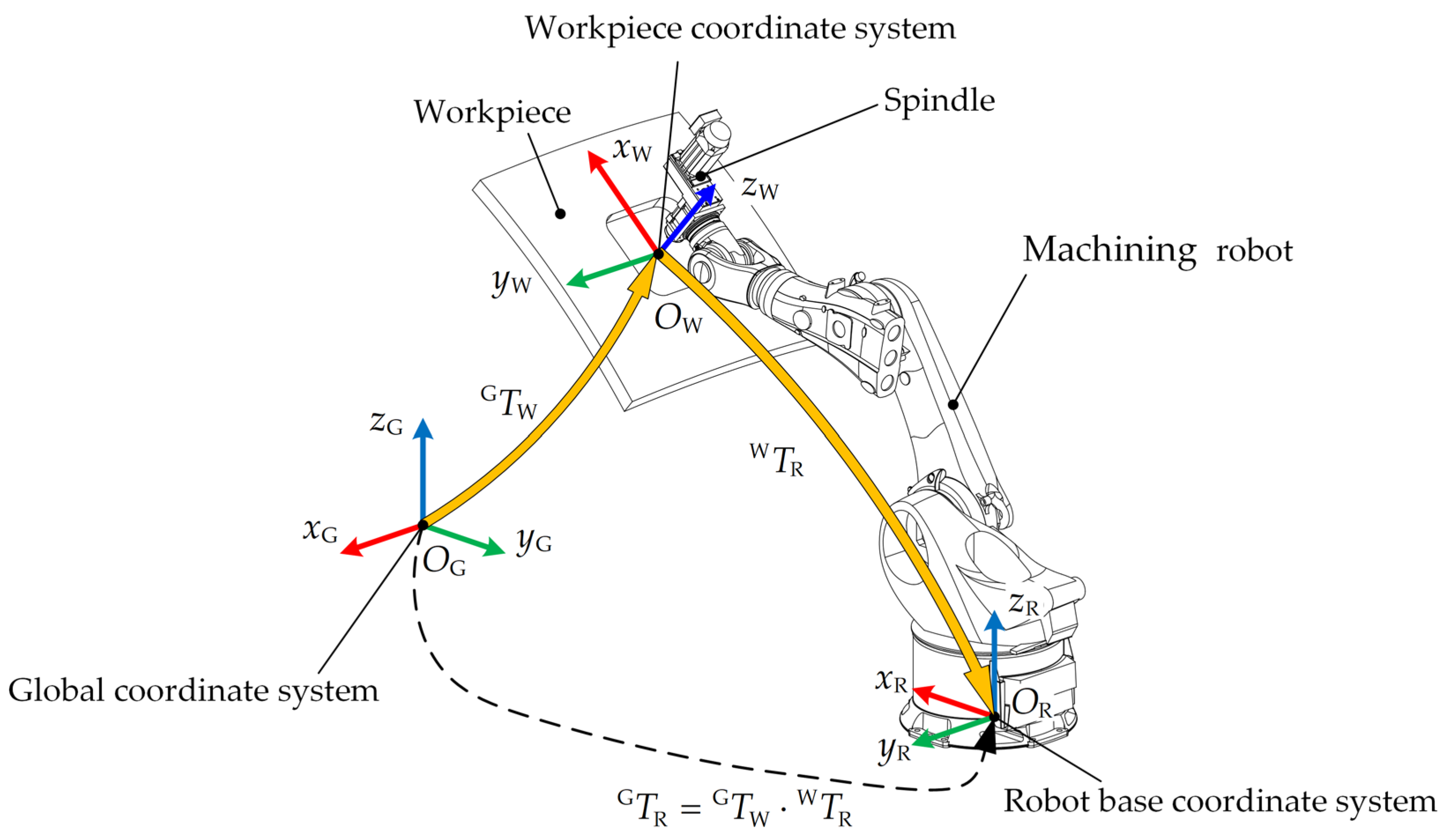
The flexible machining system, as shown in Figure 1, consists of the workpiece, the spindle, and the machining robot. The global coordinate system {G} in the machining system is established, and its origin is fixed at the geometric center of the processed part or the track center of a movement component. The workpiece coordinate system {W} is attached to the processed area. The coordinate origin of {W} is usually the geometric center of the processed feature (such as a hole or plane), and $z_{\mathrm{w}}$-axis is perpendicular to the feature plane. The spindle coordinate system {S} coincides with {W}, and the spindle is fixed on the end-effector of the robot. By establishing ${}^{\mathrm{G}}T{}_{\mathrm{R}}$, the homogeneous transformation matrix, between {S} and the robot base coordinate system, {R}, the robot base coordinate system {R} can be obtained.

The homogeneous transformation matrix ${}^{\mathrm{G}}T{}_{\mathrm{W}}$ is derived from the relative position and posture of the processed feature on the component. Additionally, the homogeneous transformation matrix ${}^{\mathrm{W}}T{}_{\mathrm{R}}$ is established according to the DH parameters of the robot. Then, by using the relationship ${}^{\mathrm{G}}T{}_{\mathrm{R}}$, as Equation (1), the position and posture of {R} in {G} is calculated, which is the target of placement planning.

$${}^{\mathrm{G}}T{}_{\mathrm{R}}={}^{\mathrm{G}}T{}_{\mathrm{W}}{}^{\mathrm{W}}T{}_{\mathrm{R}}$$

(1)

Assuming that the stiffness of the tool handle and the robot foundation remain constant, and ignoring the stiffness of each arm of the robot, the stiffness of the end-effector of the robot only depends on the stiffness of each joint. The end-effector loaded with a static force easily results in the angular displacement of the joint, causing the displacement of the spindle and reducing the machining accuracy. Based on the assumption of small deformation, the displacement of the force acting point can be ignored, namely, the joint angle is constant. Furthermore, taking the rotation joint angles and the stiffness of the end-effector as the design variable and the objective function, respectively, their mapping relationship can be established. By finding the optimal solution of joint rotation angles, we can finally calculate the optimal solution of placement for the machining robot.

3. Kinematic Model of Flexible Machining System

As the basis of placement planning, the kinematics of the machining robot are analyzed minutely in this section. According to the DH method, the coordinate frames are firstly established, and then the corresponding homogeneous transformation matrices are presented.

3.1. Coordinate Systems of Workpiece and Robot

Based on the above abstract model, in this paper, we take the milling hole processing of the large spherical shell as an example. Each coordinate system is established in Figure 2. {G} and {W} are, respectively, located at the center of the spherical shell and processed feature. The tool holder coordinate system {−1} coincides with {W}. The spindle coordinate system {S}, also recorded as {0}, is located at the intersection of the spindle axis and the robot A6 axis. The coordinate systems of each joint of the robot, labeled {1}~{6}, are determined according to the DH method. It is worth noting that the joint coordinate frame {6} is the robot base coordinate system {R}, whose origin is the intersection of the robot A1-axis and the foundation plane of the robot.

We selected a KUKA KR500 robot with 6 degrees-of-freedom (DOFs) as the machining device. In Figure 2, $\rho$ is the outer surface radius of the processed feature, and $\phi$ is the latitude of the geometric center of the feature. The angle range of each joint of the robot is marked as ${\theta }_i\in [{\theta }_{i\min },{\theta }_{i\max })$. The DH parameters of the robot are ${\theta }_i$, ${\alpha }_{i-1}$, $d_i$, and $a_{i-1}$, in which ${\theta }_i$ is the rotation angle from $x_{i-1}$-axis to $x_i$-axis with $z_i$ as the rotating axis, and ${\alpha }_{i-1}$ is the rotation angle from $z_{i-1}$-axis to $z_i$-axis with $x_{i-1}$ as the rotating axis, $d_i$ is the distance from $x_{i-1}$-axis to $x_i$-axis along $z_i$-axis, and $a_{i-1}$ is the distance from $z_{i-1}$-axis to $z_i$-axis along $x_{i-1}$-axis.

3.2. Homogeneous Transformation Matrices

The homogeneous transformation matrix from the {G} to {W} established according to the position and posture of the feature is expressed as:

$${}^{\mathrm{G}}T{}_{\mathrm{W}}=\left[\begin{array}{cccc}& {}^{\mathrm{G}}R{}_{\mathrm{W}}& & {}^{\mathrm{G}}P{}_{\mathrm{W}\mathrm{org}}\\ 0& 0& 0& 1\end{array}\right]$$

(2)

where ${}^{\mathrm{G}}R{}_{\mathrm{W}}$ and ${}^{\mathrm{G}}P{}_{\mathrm{W}\mathrm{org}}$ represent rotation matrix translation vector from {G} to {W}, respectively, and are shown as follows.

$${}^{\mathrm{G}}R{}_{\mathrm{W}}=\left[\begin{array}{ccc}0& \sin \phi & \cos \phi \\ -1& 0& 0\\ 0& -\cos \phi & \sin \phi \end{array}\right]$$

(3)

$${}^{\mathrm{G}}P{}_{\mathrm{W}org}={\left[\begin{array}{ccc}\rho \cos \phi & 0& \rho \sin \phi \end{array}\right]}^T$$

(4)

The homogeneous transformation matrix from {−1} to {0} is recorded as ${}^{-1}T{}_0$, and that of each joint is marked as ${}^{0}T{}_1$~${}^{5}T{}_6$. The corresponding homogeneous transformation matrices can be described as:

$${}^{i-1}T{}_i=\left[\begin{array}{cccc}& {}^{i-1}R{}_i& & {}^{i-1}P{}_{i\mathrm{org}}\\ 0& 0& 0& 1\end{array}\right]\left(i=0,1,\dots ,6\right)$$

(5)

where ${}^{i-1}R{}_i$ and ${}^{i-1}P{}_{i\mathrm{org}}$ mean rotation matrix and translation vector from {i} to {i − 1}, respectively. The expressions are as follows.

$${}^{i-1}R{}_i=\left[\begin{array}{ccc}\cos {\theta }_i& -\sin {\theta }_i& 0\\ \sin {\theta }_i\cos {\alpha }_{i-1}& \cos {\theta }_i\cos {\alpha }_{i-1}& -\sin {\alpha }_{i-1}\\ \sin {\theta }_i\sin {\alpha }_{i-1}& \cos {\theta }_i\sin {\alpha }_{i-1}& \cos {\alpha }_{i-1}\end{array}\right]$$

(6)

$${}^{i-1}P{}_{iorg}={\left[\begin{array}{ccc}{a}_{i-1}& -d_i\sin {\alpha }_{i-1}& d_i\cos {\alpha }_{i-1}\end{array}\right]}^{\mathrm{T}}$$

(7)

By using the chain rule, the homogeneous transformation matrix from {G} to {i} can be obtained:

$${}^{\mathrm{G}}T{}_i={}^{\mathrm{G}}T{}_{-1}\cdot {\displaystyle \prod _{j=0}^i{}^{j-1}T{}_j}=\left[\begin{array}{cccc}& {}^{\mathrm{G}}R{}_i& & {}^{\mathrm{G}}P{}_{i\mathrm{org}}\\ 0& 0& 0& 1\end{array}\right]$$

(8)

where ${}^{\mathrm{G}}R{}_i$ and ${}^{\mathrm{G}}P{}_{i\mathrm{org}}$ are the rotation matrix and the translation vector from {G} to {i}, respectively.

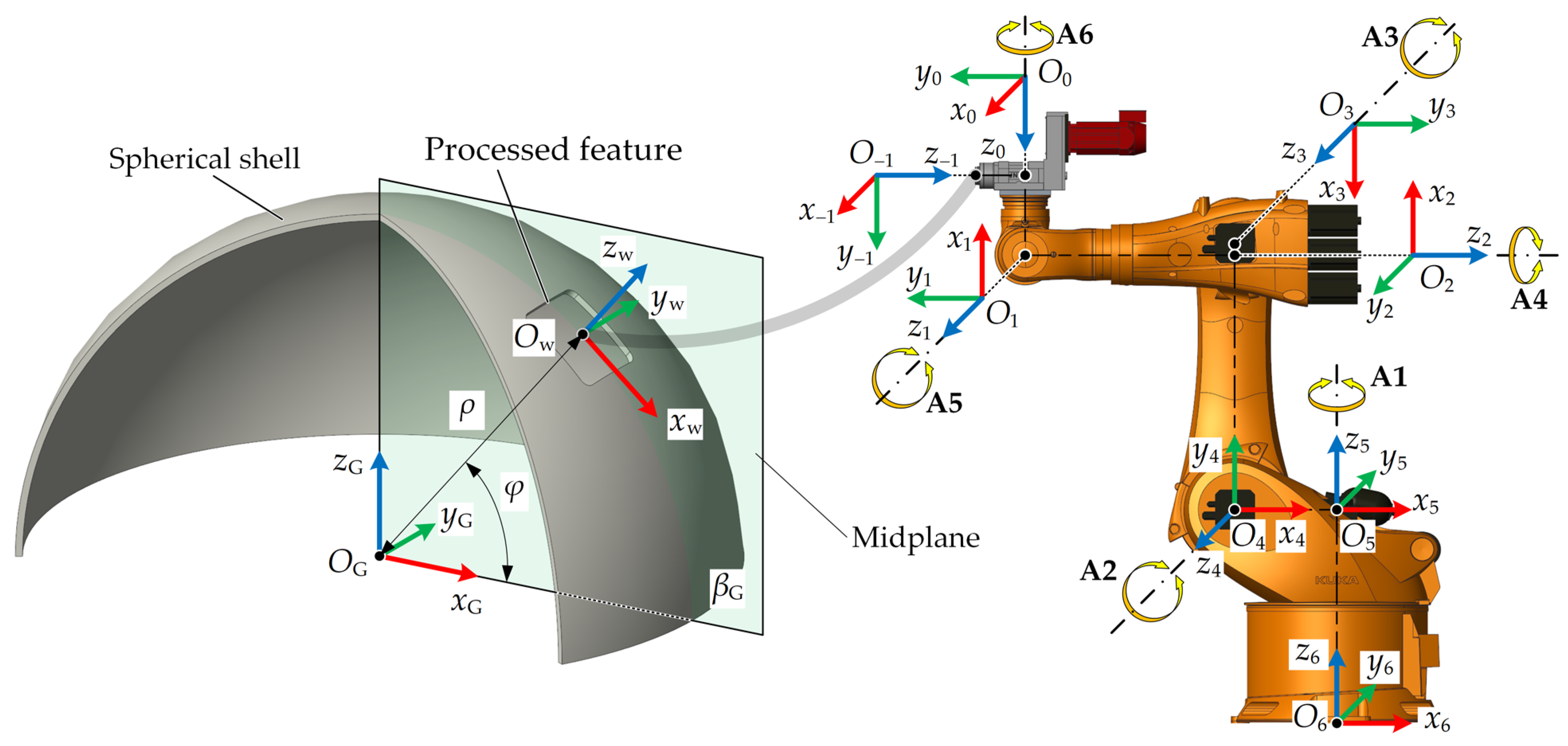
4. Center-Reachable Placement Space Meeting Motion Constraints

In this section, the center point of the processed feature is selected to evaluate the reachability performance of the machining robot. The horizontal constraint of the robot base is proposed as firstly based on the rotation angles. Subsequently, to avoid the physical interference between the robot and workpiece, collision-free constraints are derived. Finally, by combining the kinematic model, the robot placement space for the center of the processed feature is obtained.

4.1. The Constraint of the Robot Base Remaining Horizontal

To ensure machining accuracy, the gravity compensation algorithm is introduced into the machining program of the system, and its calculation premise is that the robot base remains horizontal.

The robot placement relies on the 6 rotational DOFs, which correspond with ${\theta }_i\left(i=0,\cdots ,5\right)$. The robot base remaining horizontal means that 2 DOFs (rotating $x_{\mathrm{G}}$-axis and rotating $y_{\mathrm{G}}$-axis) are constrained. Namely, two joint angles of non-parallel axes are calculated with the geometric relationship determined by other joint angles. In this paper, ${\theta }_2$ and ${\theta }_4$ are the object to calculate, while ${\theta }_0$, ${\theta }_1$ and ${\theta }_3$, being the basis of calculation, are arbitrary within their respective ranges.

Based on the given values of ${\theta }_0$ and ${\theta }_1$, the position and posture of coordinate system {1} can be obtained according to Equation (8).

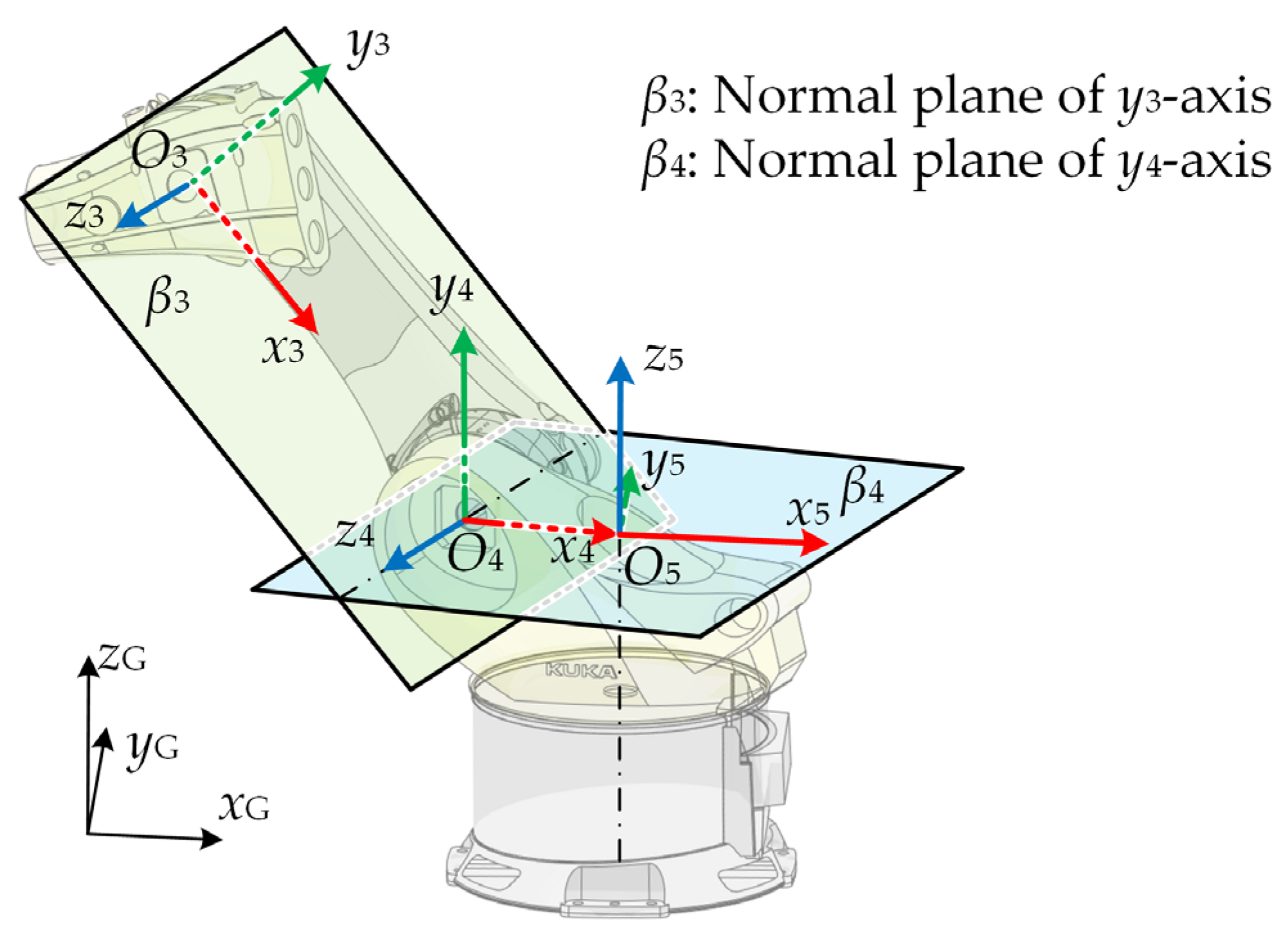
As shown in Figure 2, the necessary condition for the robot base remaining horizontal (i.e., $z_5$-axis and $z_6$-axis remaining vertical) is that the coordinate axis $z_4$-axis remains horizontal, namely, $z_3$-axis and $y_2$-axis are horizontal. Thus, ${\theta }_2$ is calculated with the postures of the target coordinate system {2} and coordinate system {1} as shown in Figure 3.

Since ${\beta }_2$ is a vertical plane, its corresponding normal can be obtained as:

$$\overrightarrow{n}={\overrightarrow{z}}_{\mathrm{G}}\times {\overrightarrow{y}}_1$$

(9)

Then ${\theta }_2$ is the dihedral angle between ${\gamma }_1$ and ${\beta }_2$, i.e.,

$${\theta }_2=\langle \overrightarrow{n},{\overrightarrow{z}}_1\rangle$$

(10)

Furthermore, combined with the value of ${\theta }_3$, the position and posture of coordinate system {3} are calculated.

As shown in Figure 4, on the premise of $z_4$-axis remaining horizontal, the sufficient and necessary condition for the robot base horizontal is that $x_4$-axis remains horizontal. Thus, the joint angle ${\theta }_4$ can be calculated.

${\theta }_4$ is the dihedral angle between ${\beta }_3$ and ${\beta }_4$. ${\beta }_4$ is horizontal, hence ${\theta }_4$ meets:

$${\theta }_4=\langle {\overrightarrow{y}}_3,{\overrightarrow{z}}_{\mathrm{G}}\rangle$$

(11)

Based on ${\theta }_2$ and ${\theta }_4$ obtained from the above analysis, $z_4$-axis and $x_4$-axis are horizontal vectors, thereby $y_4$-axis is perpendicular to the horizontal. $z_5$-axis and $z_6$-axis are parallel to $y_4$-axis, namely, the robot base plane remains horizontal.

4.2. The Constraint of Physical Collision-Free

According to the definition of the parameters, ${}^{\mathrm{G}}P{}_{i\mathrm{org}}$ can reflect the position and posture of each robot arm. For the processed component of the spherical shell, theoretically, the distance from ${}^{\mathrm{G}}P{}_{i\mathrm{org}}$ to $O_{\mathrm{G}}$ only needs to be longer than the outer diameter of the processed spherical shell. Considering the structural size of robot arms, the safety distance $\Delta \rho$ is introduced. For each arm of the robot, $\Delta \rho$ is the minimum distance from the coordinate origin to the arm surface. Then, for ${}^{\mathrm{G}}P{}_{i\mathrm{org}}$, the following condition must be satisfied:

$$\overline{{}^{\mathrm{G}}P{}_{i\mathrm{org}}{O}_{\mathrm{G}}}>\rho +\Delta \rho ,\left(i=0,1,\cdots ,6\right)$$

(12)

For the machining project involved in this paper, the excessive value of ${\theta }_5$ (rotation angle in the negative direction of the robot A1-axis) will lead to a collision between the robot body and the positioning platform, as illustrated in Figure 5.

Considering the positioning platform, $x_5$-axis is in the same direction as $x_{\mathrm{G}}$-axis, thus the angle of A1-axis is:

$${\theta }_5=\langle {\overrightarrow{x}}_4,{\overrightarrow{x}}_G\rangle \in [{\theta }_{5\min },{\theta }_{5\max })$$

(13)

Therefore, by combining the two conditions as Equations (12) and (13), the constraint of physical collision-free can be derived.

4.3. Placement Space of Robot

The set of the vector assembled by robot joint angles meeting the above constraints is named as Center-Reachable Joint Space (CRJS), which is joint space according to the constraints of position and posture. Through the joint coordinates in CRJS, each ${}^{\mathrm{G}}P{}_{6\mathrm{org}}$, coordinate of the robot position in the global coordinate system, is calculated (in Equation (8)) and marked as $\left(s_x,s_y,s_z\right)$. Correspondingly, the solution set of $\left(s_x,s_y,s_z\right)$ is named as Center-Reachable Placement Space (CRPS), which is placement space according to the constraints of position and posture.

5. Boundary-Reachable Placement Space Meeting Reachability Constraints

The above constraints can only meet the reachability of the robot to the feature center. On this basis, the placements also need to meet the reachability of any point on the feature. The intersection line of the envelope surface of CRPS and the parallel plane of the feature is a convex envelope line, so reachability to any point of the feature is equivalent to reachability to the boundary point of the feature.

Considering the feature shown in Figure 6, any point in CRPS can satisfy the reachability of point $O_{\mathrm{C}}$, the geometric center of the processed feature $ABCD$. Take any point $P_1$ in CRPS and determine the points $A_1$, $B_1$, $C_1$, and $D_1$ around $P_1$. The following constraint for point $D_1$ should hold:

$$\overrightarrow{P_1{D}_1}=-\overrightarrow{O_{\mathrm{C}}D}$$

(14)

According to the geometric relationship of parallelogram PD₁O_CD, point $D_1$ also should match the following condition:

$$\overrightarrow{D_1{O}_{\mathrm{C}}}=\overrightarrow{P_{1}D}$$

(15)

Similarly, points $A_1$, $B_1$, and $C_1$ are the same as point $D_1$.

As point $D_1$ is within CRPS, the robot can meet the reachability from point $D_1$ to point $O_{\mathrm{C}}$, and the robot can reach point $D_1$ from point $P_1$ in the same posture. Point $C_1$ is the same as point $D_1$. However, $A_1$ and $B_1$ are opposite to $D_1$. Therefore, the robot cannot reach points $A_1$ or $B_1$ from point $P_1$. Namely, position $P_1$ cannot satisfy reachability constraints.

However, points $A_2$, $B_2$, $C_2$, and $D_2$ are all within CRPS. Therefore, the robot can meet the reachability from point $P_2$ to points $A_2$, $B_2$, $C_2$, and $D_2$, namely, position $P_2$ is an available base placement.

The placement space fulfilling the reachability condition is named as Boundary-Reachable Placement Space (BRPS), which is filtered from CRPS through the above methods. Therefore, the joint space corresponding to BRPS is Boundary-Reachable Joint Space (BRJS). Since CRPS is the result calculated based on some arbitrary values (${\theta }_0$, ${\theta }_1$, and ${\theta }_3$), it is surely a non-empty set. For this reason, if BRPS is an empty set, it is attributed to reachability constraints, then recalculation is required after dividing the feature.

6. Stiffness Analysis and Placement Optimization of Robot

As machining accuracy is directly related to the stiffness of the robot, in this section, robot stiffness is further studied by establishing the mapping between joint force and robot posture, and the optimization method based on the global maximum stiffness is given.

6.1. Joint Force of Robot

As the interaction force between adjacent robot arms is an internal force, the relative mechanical characteristics between the end-effector and the base are separate from the position of the action point of the force at each joint. To facilitate the research, the action point of the force at each joint is selected at the origin of the joint coordinate system.

The transformation of generalized force between joint i and joint i + 1 is:

$$\left[\begin{array}{c}{\overrightarrow{F}}_{i+1}\\ {\overrightarrow{M}}_{i+1}\end{array}\right]=\left[\begin{array}{cc}{}^{i+1}R{}_i& 0\\ \left[\begin{array}{ccc}0& -{}^{i+1}p{}_{iz}& {}^{i+1}p{}_{iy}\\ {}^{i+1}p{}_{iz}& 0& -{}^{i+1}p{}_{ix}\\ -{}^{i+1}P{}_{iy}& {}^{i+1}P{}_{ix}& 0\end{array}\right]\cdot {}^{i+1}R{}_i& {}^{i+1}R{}_i\end{array}\right]\cdot \left[\begin{array}{c}{\overrightarrow{F}}_i\\ {\overrightarrow{M}}_i\end{array}\right]\left(i=-1,0,1,\dots ,5\right)$$

(16)

where ${\overrightarrow{F}}_i$ and ${\overrightarrow{M}}_i$, respectively, represent the force and the torque in joint i.

Each joint has only one rotational DOF around the z-axis, thus only $M_{iz}$, the torque to $z_i$-axis in joint i, has an impact on the stiffness of the end-effector. The vector assembled by $M_{iz}$ is recorded as $\tau$.

$$\tau ={\left[\begin{array}{cccc}{M}_{1z}& M_{2z}& \cdots & M_{6z}\end{array}\right]}^{\mathrm{T}}$$

(17)

6.2. Optimization of Robot Placement

For the posture of the robot corresponding to the joint angle $\theta$, the joint angle deviation $\Delta \theta$ is:

$$\Delta \theta =K_{\theta }{}^{-1}\cdot \mathbf{\tau }$$

(18)

where $K_{\theta }$ means the robot joint stiffness matrix.

Then, under the joint angle deviation $\Delta \theta$, the expression of the displacement deviation of the end-effector in coordinate system {R} is recorded as ${}^{\mathrm{R}}\Delta P$:

$$\left[\begin{array}{c}{}^{\mathrm{R}}\Delta P\\ 0\end{array}\right]={}^{\mathrm{R}}T{}_0\left(\theta \right)\cdot \left[\begin{array}{c}{}^{0}P{}_{-1\mathrm{org}}\\ 1\end{array}\right]-{}^{\mathrm{R}}T{}_0\left(\theta +\Delta \theta \right)\cdot \left[\begin{array}{c}{}^{0}P{}_{-1\mathrm{org}}\\ 1\end{array}\right]$$

(19)

The expression of the displacement deviation in coordinate system {−1} is marked as ${}^{-1}\Delta P$:

$$\left[\begin{array}{c}{}^{-1}\Delta P\\ 1\end{array}\right]=\left[\begin{array}{c}{}^{-1}\Delta p_x\\ {}^{-1}\Delta p_y\\ {}^{-1}\Delta p_z\\ 1\end{array}\right]={}^{-1}T{}_{\mathrm{R}}\left(\theta \right)\cdot \left[\begin{array}{c}{}^{\mathrm{R}}\Delta P\\ 1\end{array}\right]$$

(20)

The displacement of the tool holder in the normal plane of $z_{-1}$-axis, $\delta \left(\theta \right)$, is taken as the index to describe the stiffness of the end-effector in the posture:

$$\delta \left(\theta \right)=\sqrt{{}^{-1}\Delta p_x{}^2+{}^{-1}\Delta p_y{}^2}$$

(21)

Generally, the stiffness of the end-effector of the robot decreases with the increase in the span from the robot base to the end-effector. Therefore, in the process of machining the whole feature, in the posture with the weakest stiffness, the end-effector must be on the feature boundary point. For the $j$th placement in BRPS, the postures to the boundary points $A$, $B$, $C$, and $D$ are determined. The angle vectors of the postures (marked as ${\theta }_{jA}$, ${\theta }_{jB}$, ${\theta }_{jC}$ and ${\theta }_{jD}$) are, respectively, used to calculate the deformations of the end-effector (${\delta }_{jA}$, ${\delta }_{jB}$, ${\delta }_{jC}$, and ${\delta }_{jD}$). The maximum value of these deformations is taken as the objective function of placement optimization:

$${\delta }_j=\max \left\{{\delta }_{jA},{\delta }_{jB},{\delta }_{jC},{\delta }_{jD}\right\},\left(j=1,2,\cdots ,n\right)$$

(22)

The minimum value ${\delta }^{*}$ is searched from ${\delta }_j\left(j=1,2,\cdots ,n\right)$, and the coordinate of the corresponding placement $S^{*}$ is the optimal solution:

$${\delta }^{*}=\underset{j}{\min }\left\{{\delta }_j\right\}$$

(23)

$$S^{*}={\left[\begin{array}{ccc}{s}_{xj}{}^{*}& s_{yj}{}^{*}& s_{zj}{}^{*}\end{array}\right]}^{\mathrm{T}}$$

(24)

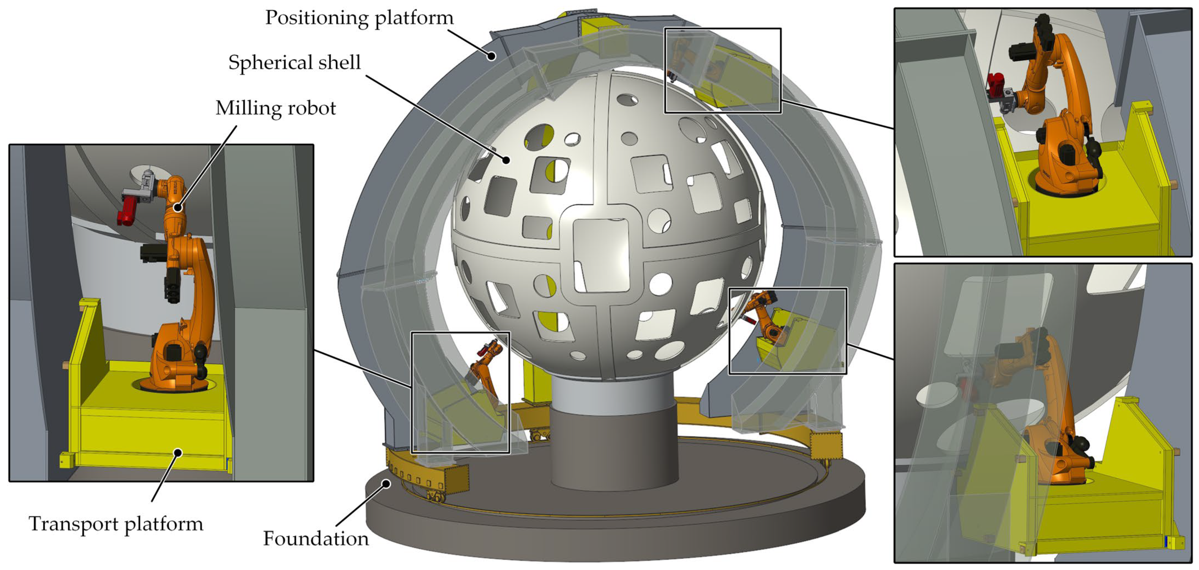
7. Calculation Case

In the project involved in this paper, the placement optimization method is used to determine the positions of the robot relative to the processed component, and the KUKA KR500 robot is adopted for the milling process. The diagram of the flexible machining system with the robot processing in different placements is shown in Figure 7.

By assembling the transport platform at the determined position between the two arch beams of the positioning platform, the robot is fixed at a determined placement. By changing the assembling position of the transport platform, the robot can shift between different latitudes. By rotating the positioning platform on the foundation, the robot can move at a constant latitude and continuously change longitude.

Comprehensive analysis of the above robot placement planning mainly includes the following steps: Firstly, the kinematic model of the machining robot is developed with the parameters of the robot and processed features. In consideration of reachability constraints, the parameters of features may need to be re-imported after dividing the features. Next, the placement spaces (CRPS and BRPS) are determined. Lastly, optimization placement is solved. The robot placement planning flow chart is illustrated in Figure 8.

7.1. Kinematics Model Parameter Inputting

For the processed large spherical shell component, the processed holes on it have different outer surface radii, shapes, positions, and sizes. The parameters of the selected KUKA robot and a specific rectangle processed hole are given in

Table 1. The parameters of the KUKA KR500 robot.

Joint i	θi	αi−1	ai−1/mm	di/mm
0	[0°, 360°)	−90°	385	400
1	[−120°, 120°)	90°	0	0
2	[0°, 360°)	90°	0	1025
3	[234°, 10°)	−90°	55	0
4	[−20°, 130°)	0°	1300	0
5	[−185°, 185°)	−90°	500	0
6	0°	0°	0	1045

and

Table 2. The position and size of the component and a specific hole.

The Radius of the Outer Surface ρ/mm	Latitude	Width/mm	Height/mm
5900	0°	2000	2700

, respectively.

After the trial calculation, for the feature shown in Table 2, in the situations of no division and dividing into two parts, BRPSs are both empty sets, while it is a non-empty set in the situation of dividing into three parts in the height direction. The following calculation is based on this condition. These parts are processed separately. The positions and sizes of the parts are given in

Table 3. The positions and sizes of the component and a specific hole (after being divided).

Part i	The Radius of the Outer Surface ρ/mm	Latitude	Width/mm	Height/mm
I	5900	8.774°	2000	900
II	5900	0°	2000	900
III	5900	−8.774°	2000	900

.

7.2. Solution of Placement Space (CRPS and BRPS)

${\theta }_0$,${\theta }_1$ and ${\theta }_3$ traverse the value range shown in Table 2, respectively, according to the given step size. ${\theta }_0\in [180°,360°)$ is a redundant range, thus ${\theta }_0$ only needs to traverse $[0°,180°)$. ${\theta }_2$, ${\theta }_4$ and ${\theta }_5$ are calculated through the geometric relationship shown in Section 4. So far, CRJS is established, and the corresponding CRPS can be solved.

For the three parts of the processed feature in Table 3, the projection of the envelope of CRPS on $x_{\mathrm{G}}{O}_{\mathrm{G}}{z}_{\mathrm{G}}$ plane and the postures of the robot under certain placements are shown in Figure 9.

The posture diagram of the robot in Figure 9 is simulated by the 3-D modeling software Creo according to the corresponding joint angles in CRJS, as below. As shown, the robot postures calculated by the model are the same as the postures simulated by the 3-D modeling software, and both of them can meet the reachability to the center of the processed feature.

Since the procedures to determine BRPS for different parts of the feature are the same, the BRPS of part II in Table 3 is calculated as a case. BRPS is filtered through the method of Section 5. The placement spaces (CRPS and BRPS) are shown in Figure 10. (a) and (b) in Figure 10 representing the projections in planes $x_{\mathrm{G}}{O}_{\mathrm{G}}{z}_{\mathrm{G}}$ and $x_{\mathrm{G}}{O}_{\mathrm{G}}{y}_{\mathrm{G}}$, respectively.

7.3. Placement Optimization

According to the experiment by Cvitanic et al. [33], through the static stiffness model which was developed with decoupled partial pose method, the joint static stiffness values are given as:

$$K_{\theta }=diag\left(\begin{array}{cccccc}8.8& 5.5& 5.3& 111& 99& 59\end{array}\right)\times {10}^5\mathrm{Nm}/\mathrm{rad}$$

(25)

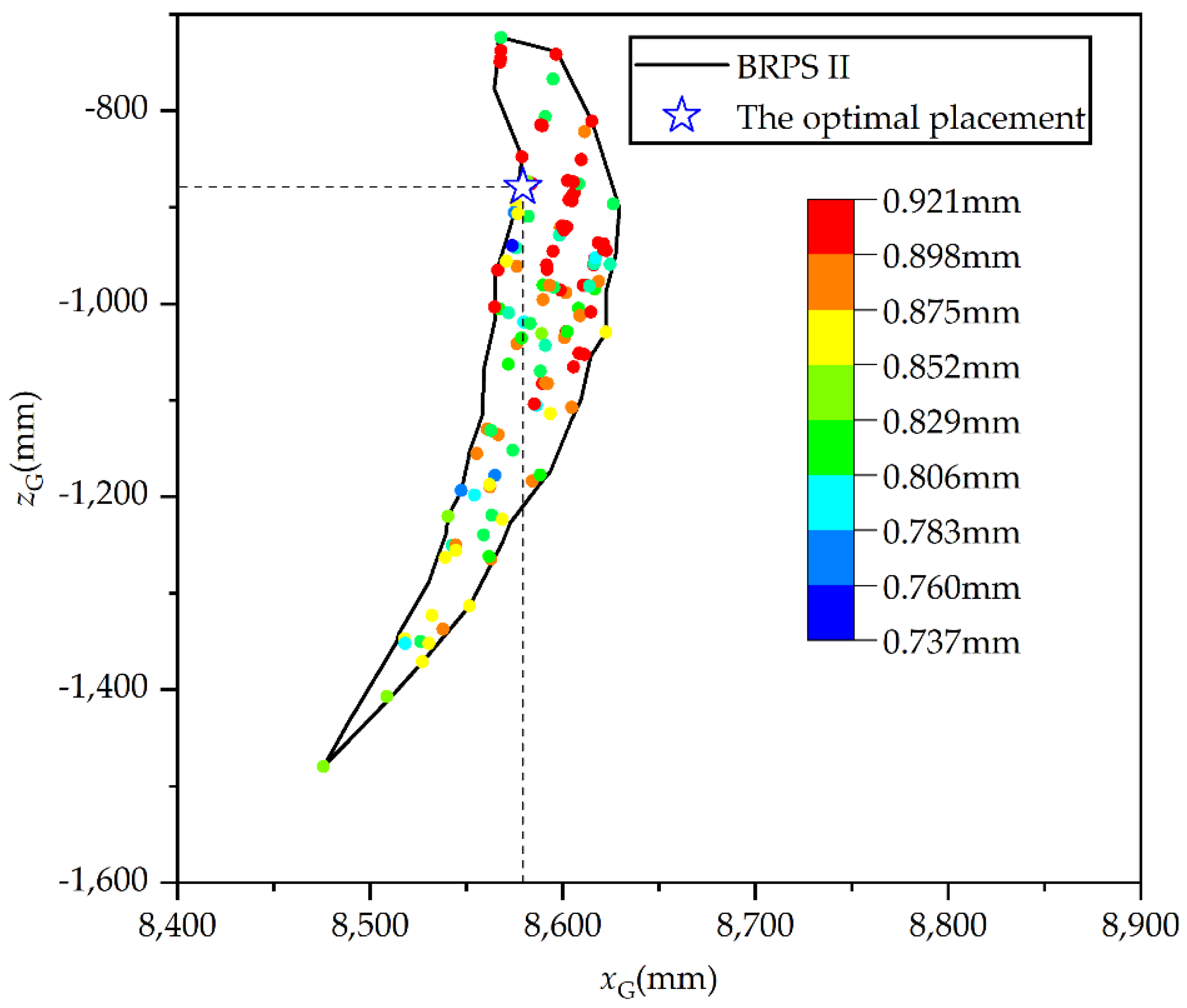
Taking feature II in Table 3 as an example, in the weak stiffness posture of the robot, under the load given in Equation (26), the distribution of static deformation $\delta$ in BRPS is illustrated in Figure 11. The workspace of the robot end-effector and processed feature are both symmetrical, so under the condition that their mid-planes coincide, i.e., machining symmetrically, the end-effector has high stiffness. Therefore, Figure 11 only shows the distribution in the mid-plane $x_{\mathrm{G}}{O}_{\mathrm{G}}{y}_{\mathrm{G}}$.

$$\{\begin{array}{c}{\overrightarrow{F}}_{-1}={[100,100,0]}^{\mathrm{T}}\mathrm{N}\\ {\overrightarrow{M}}_{-1}={[0,0,{10}^3]}^{\mathrm{T}}\mathrm{N}\cdot \mathrm{mm}\end{array}$$

(26)

In BRPS, in total, the stiffness decreases with the increase in distance in $x_{\mathrm{G}}$-axis direction. The maximum and minimum values of deformation of the end-effector are 0.921 mm and 0.737 mm, respectively. However, the stiffness may differ significantly with the robot postures even if the placements are approached. Therefore, the distribution is greatly discontinuous. The optimal placement $S_{\mathrm{II}}^{*}$ is (8579, 0, −879) and the minimum ${\delta }^{*}$ is 0.737 mm.

7.4. Model Validation

The reachability of the robot end-effector to the boundary of the processed feature can be confirmed by the robot postures in Figure 10, which proves the correctness of the robot kinematics model. So, the feasibility of placement space can be inferred.

The deformation of the end-effector caused by the stiffness of each arm of the robot is much less than that caused by the joint stiffness. In addition, in the static stiffness identification experiment, deformation of the robot arms is coupled to the deformation of the end-effector, namely, the stiffnesses of the robot arms have been somewhat considered in the results of stiffness identification. Therefore, ignoring the stiffness of the manipulator is a feasibly simplified scheme. On the other hand, the servo system of robot joints involves servo motors and different types of reducers, for which stiffness models are very complex. According to the existing research, it is difficult to achieve accurate modeling of a joint servo system. Joint stiffness is the identification result of the robot in the normal working range, which is represented in the range. The postures of the robot involved in this paper are within the normal working range, so it is a reasonable assumption to regard the joint stiffness as a constant value.

The multi rigid body static model of the robot is established in ANSYS Workbench. Fixed constraints are added to the foundation of the robot, and torsion springs with certain stiffnesses (as Equation (25)) are added to the rotating pairs of each joint. Force (as Equation (26)) is applied to the end-effector. Under the four postures of part II boundary points A, B, C, and D, the calculation results and simulation results of the static deformation of the end-effector in the normal plane are, respectively, shown in

Table 4. The static deformation of the end-effector.

	Calculation Results	Simulation Results	Error
${\delta }_A^{*}$	0.730	0.728	0.19%
${\delta }_B^{*}$	0.730	0.728	0.22%
${\delta }_C^{*}$	0.737	0.733	0.58%
${\delta }_D^{*}$	0.723	0.722	0.18%

.

The differentials between calculation results by model and simulation results by the software are in the micro-level. The errors of the model are less than 0.6%.

Thus, the correctness of the calculation model can be validated, and the static deformation of robots in other positions and postures can be calculated through the model, so as to validate the correctness of the optimal solution.

8. Conclusions

Aimed at obtaining the optimal stiffness of the machining robot, in this paper, a robot placement planning strategy for a large processed component was developed. The kinematic model of the machining robot was established by firstly utilizing the DH method. Subsequently, according to motion constraints and spatial reachability, the CRPS and BRPS were proposed. On the basis of the established relationship between joint force and robot posture, the global stiffness optimization method was presented, which ensured maximized stiffness and high accuracy throughout the whole machining process. A flexible machining system for a large processed component was analyzed as an example. The finite element simulation results were in good agreement with the proposed optimization method, demonstrating that it was effective in improving machining robot stiffness and enhancing machining quality. In future work, we will focus on the physical machining system and will evaluate the actual effect of the optimization algorithm.