Abstract
The aeroengine industry has set strict upper limits for assembly errors in rotor-connecting processes, because assembly errors significantly affect aeroengine stability. Applications of multi-axis mechanisms have the potential to solve the low efficiency of traditional manual connection processes. However, multiple error sources are simultaneously introduced. Thus, an accurate prediction method of rotor assembly error considering multiple error sources is of vital importance, by which the applicability of the new mechanism to rotors can be tested. In this study, a new prediction method for rotor assembly errors is proposed based on the use of a novel multi-axis measuring and connecting mechanism. First, the error propagation among the rotor errors, measurement errors, mechanism errors, and mounting errors is analyzed. Second, reasonable characterization models for these error sources are established using homogeneous transformation matrices. Third, based on the abovementioned error models, a new rotor assembly error prediction algorithm is constructed. It is highly consistent with the actual connection processes. Finally, verification experiments are conducted. The experimental results show that deviation rates of the average values of six types of assembly errors relative to the predictions are all lower than 14%. The proposed prediction method has acceptable accuracy and practical significance.
1. Introduction
The assembly error of an aeroengine rotor assembly (e.g., compressor and turbine) refers to the relative deviation or deflection between the specific structures on different rotor parts after the connecting processes [1]. Manufacturing enterprises have set strict upper limits for rotor assembly errors, because they significantly affect the wear, vibration, and aerodynamic performance of the final assembly [2,3]. However, manual operation using simple mechanisms is still widely used. Each assembly error is guaranteed to be lower than the corresponding upper limit through multiple trial connecting processes and repeated measurements, because the qualification rate of a single trial connecting process is only lower than 50%. To address the low quality and efficiency of the traditional manual method, an automated six-axis numerical control (NC) mechanism for rotor position and pose adjustment and connection, as well as a three-axis coordinate measuring machine (CMM), can be applied in modern aeroengine assembly lines. Servo linkage axes can completely replace manual measuring and connecting motions on multiple spatial degrees of freedom with higher motion accuracy [4]. However, a key issue is introduced: to verify the applicability of a newly designed multi-axis measuring and connecting mechanism to rotors with different accuracy levels, an accurate prediction method of rotor assembly errors is highly necessary.
Studies have been devoted to proposing prediction methods for assembly errors using various mathematical models [5,6,7,8,9,10]. Sun et al. used a particle swarm optimization neural network to propose a prediction method for the concentricity and perpendicularity of aeroengine multistage rotors [11]. Ding et al. predicted the overall concentric performance of rotors with optimized connection angles based on the Jacobian Torsor model [12]. Zhang et al. predicted assembly errors by mainly considering the plane geometric form errors of multiple parts based on the kernel function [13]. Their studies achieved reasonable accuracy in predicting assembly errors, but only considered a specific type of main error source in the assembly process.
However, owing to the use of complex multi-axis measuring and connecting mechanisms, different types of error sources are introduced into the assembly errors. The characterization and propagation of the error sources should be clarified in the prediction method to improve the prediction accuracy. The main error sources include: (1) the shape and position errors of the rotors [14,15,16,17]—the errors at the flange end faces and rabbet joint structures affect the relative position and pose between adjacent rotors. The errors at the positioning structures for other functional parts (e.g., bearings, couplings, and sealing discs) have direct impacts on the assembly errors; (2) measurement errors [18,19,20,21]—there are errors in the fitted geometric features owing to the deviations between the measured points and their nominal locations when measuring the connection structures and positioning structures; (3) mechanism errors [22,23,24]—there are relative motion and static errors between each two adjacent axes in the six-axis mechanism for adjusting and connecting rotors, which cause the position and pose error of the end fixture relative to the fixed base after the connection motion; and (4) mounting errors [25,26,27]—there are errors of the clamped rotor relative to its nominal position and pose in the clamping fixture on the six-axis mechanism.
Thus, the rotor assembly error prediction algorithm should integrate and simulate multiple types of error sources. The construction of the prediction algorithm faces two difficulties. First, a unified mathematical model should be used to characterize different errors, as well as to describe the error propagation among them. Second, various error sources include a lot of random error items. The initial conditions of connecting processes are also random. The prediction algorithm should be able to calculate different statistical inputs and outputs. In addition, the prediction algorithm flow should be highly consistent with the actual connection processes.
To solve the first difficulty, general homogeneous coordinate transformation matrices could be used as the unified mathematical model to represent different types of errors. A general 4 × 4 homogeneous coordinate transformation matrix clarifies the relative spatial relationship between the coordinate systems A and B in two geometric features [28,29]. The column matrices , , and in represent the pose of B relative to A, and the column matrix represents the corresponding relative position. The error propagation can be described using the error transformation matrix . In addition, the homogeneous matrices are also convenient for the operation in a complex algorithm [30].
In previous studies on modeling different types of errors, homogeneous coordinate transformation matrices show universality. (1) With regard to shape and position errors, Whitney et al. applied homogeneous coordinate transformation matrices to represent both the nominal relations between parts and variations caused by shape and position errors allowed by the tolerances [31]. Wu et al. used homogeneous coordinate transformation matrices for the position calculation of geometric features in assembly tolerance analysis [32]; (2) With regard to measurement errors, Zhang et al. established an error transfer model of an aeroengine rotor measuring machine using homogeneous coordinate transformation matrices [33]. Zhou et al. used homogeneous coordinate transformation matrices to illustrate the common points and control points for measuring aerospace components [34]. Similarly, the measured and fitted geometric features relative to their nominal position and pose can also be expressed by homogeneous coordinate matrices [35,36,37]. Calvo et al. proposed a new minimum zone fitting algorithm for sphericity according to the measuring points containing measurement errors using homogeneous coordinate transformation matrices [38]; (3) With regard to mechanism errors, the relative position and pose with errors between each two adjacent axes in the multi-axis mechanism can be expressed by the multiplications of homogeneous coordinate transformation matrices under a specific law, and the actual position and pose of the terminal fixture containing all mechanism errors is obtained after multi-axis transmissions. The spatial mechanical error can be accurately determined using the modified D-H method, which comprises homogeneous coordinate transformation matrices with multiple parameters [39,40]. Zhou et al. proposed a general mathematical model for analyzing the forward kinematics and errors of a six-axis platform based on the D-H method with multiple geometric parameters [41]. The error differential matrix , based on the D-H method in the multi-axis mechanism, clarifies the value and direction of the synthetic error between the two axes [42,43]. Chen et al. regarded the error of a single motion axis as a differential movement and then calculated the tool pose error in a four-axis mechanism using error differential matrices [44]; (4) With regard to mounting errors, the error of the rotor relative to its clamping fixture on the six-axis mechanism is a static position and pose error, which can also be calculated using homogeneous coordinate transformation matrices [45,46,47]. In general, it can be seen that a specific type of error could be described using the corresponding modified homogeneous coordinate transformation matrices. However, only a few studies have applied them to model various errors in an assembly process. Homogeneous coordinate transformation matrices and error differential matrices have the potential to compose the unified error characterization and propagation mathematical models in the rotor assembly prediction method, when using a complex multi-axis measuring and connecting mechanism.
To solve the second difficulty, the Monte Carlo method is applicable to numerical simulations of various types of statistical inputs and outputs of errors [48,49,50]. There are system and random error items in each error source during the rotor-connecting processes. In practical applications, system errors are determined through repetitive experiments, and removed through accuracy adjustment or NC compensation [51,52]. However, random errors fluctuate within certain ranges according to the accuracy of the corresponding processes or mechanisms [53,54]. An accurate error value and direction cannot be determined before each connecting process. Therefore, the Monte Carlo method can be used for the statistical characterization and simulation of random errors [55,56]. Tang et al. introduced the positioning, straightness, pose, and axial errors of each axis of a six-axis mechanism into the Monte Carlo method to analyze the error sensitivity [57]. Liu et al. presented an error propagation analysis method to estimate the final integrated error of an H-drive stage using the Monte Carlo method, in which a variety of error sources including straightness, thermal, deformation, and bearing gap change errors are sampled from their distributions as the inputs respectively [58]. Thus, the Monte Carlo method could be the main process framework of the prediction algorithm for rotor connection processes, in which several types of errors are input, calculated and output. Furthermore, in contrast to existing studies, the algorithm process should simulate the actual measuring and connecting processes when using an automated multi-axis mechanism. For example, the new position and pose of the last connected rotor are measured by the CMM to guide the connecting motion of the next rotor. The flow of the prediction algorithm should be consistent with these corresponding actual processes to ensure simulation accuracy.
In this study, a systematic investigation was carried out to propose a prediction method of the rotor assembly error considering multiple error sources, based on the use of a novel multi-axis measuring and connecting mechanism. First, four main error sources that affect rotor assembly errors were investigated. The error propagation among them was indicated by the general homogeneous coordinate transformation matrices and error transformation matrices. Second, the characterization models for the four error sources were established. The rotor shape and position errors at the flange end faces, rabbet joint structures and positioning structures were modeled, and they were related to the corresponding tolerances. The measured point coordinates affected by the measurement errors were generated when measuring the annular end faces and cylindrical faces on the rotor connection and positioning structures. Then, the position and pose matrices representing the measured geometric features were derived. The errors of the six-axis rotor connecting mechanism were derived based on the modified D-H method with five parameters, and the mounting errors were modeled using the differential matrix. Subsequently, the rotor assembly position and pose errors were derived. Third, a rotor assembly error prediction algorithm was constructed based on the abovementioned error models using the Monte Carlo method. The algorithm procedure was highly consistent with the actual connection processes. The measured errors, or errors sampled from their distributions, as well as the initial conditions, were input into the algorithm. The outputs were used to analyze the applicability of the new multi-axis mechanism to the rotors with different accuracy levels. Finally, connection experiments were performed using three aeroengine rotor assemblies to verify the proposed prediction method.
This paper is organized as follows. In Section 2, the propagation of the error sources of rotor assembly errors is derived; in Section 3, the specific mathematical models of the different error sources are established; in Section 4, a rotor assembly error prediction algorithm is constructed, and the results are analyzed; in Section 5, the verification experiments are performed; and in Section 6, the conclusions are presented.
2. Classification and Propagation of the Error Sources in Rotor Connecting Processes
The main error sources that affect the final assembly errors in the rotor connecting processes include: shape and position errors, which are related to the connection structure of the rotors; measurement errors when measuring rotor initial position and pose, as well as final assembly errors; mechanism errors of the six-axis mechanism for adjusting and connecting rotors; and mounting errors of the rotor clamping fixture on the six-axis mechanism, as shown in Figure 1.
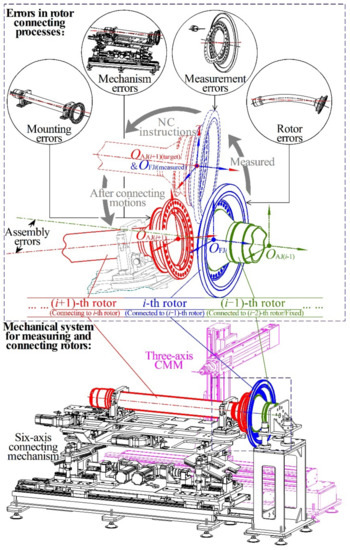
Figure 1.
Schematic of error classification and propagation in rotor connecting processes.
With regard to the propagation of these four types of errors, the shape and position errors of the rotors are direct influencing factors. This is because assembly errors are defined by the relative positions and poses of some specific positioning structures on different rotors. The shape and position errors directly determine the deviations and deflections of these specific positioning structures relative to the geometric references. In addition, the shape and position errors on rotor connecting structures, for example, flanges and rabbets, lead to deviations and deflections between adjacent rotors. At the beginning of the connecting process, the initial position and pose of the rotor should be measured, that is, the flange end face, center of the rabbet joint structure, and center of the datum connection hole (for threaded fasteners, dowel pins, etc.). In the measurement processes, owing to errors in the acquisition of point cloud coordinates, the fitted geometric features deviate and deflect from the actual features. These fitted geometric features with measurement errors are input into the NC system of the six-axis mechanism to guide the clamped rotor to make the adjusting and connecting motions. At the end of the connecting process, the relative positions and poses of the specific structures of the different rotors should be measured. The measurement errors are introduced into the assembly errors again. When the six-axis mechanism receives the linkage motion NC instruction, the static and motion errors between adjacent axes are transmitted from the fixed base of the mechanism to the end fixture. In addition, there is a mounting error in the clamped rotor relative to its nominal mounting position and pose. The mounting error and six-axis mechanism error together cause a synthetic error between the final actual position and pose of the clamped rotor and its target position and pose determined by the NC instruction.
Error propagation is described by position and pose representation matrices and error transformation matrices based on homogeneous coordinate transformations. The assembly error can be expressed using the relative position and pose transformation matrix , which represents the transformation from the jA-th positioning structure on the aft iA-th rotor to the jF-th positioning structure on the fore iF-th rotor.
where is the transformation matrix from B to Eij, superscript B represents the basic coordinate system; and subscript Eij represents the j-th positioning structure on the i-th rotor.
is derived as follows:
where the subscripts (or superscripts) FJi and AJi represent the fore and aft rabbet joint structures on the i-th rotor, respectively.
Shape and position errors of rotors are introduced into Equation (2).
where and represent the shape and position error transformation matrices from AJi to FJi and Eij, respectively.
The matrix in Equation (2) indicates the transformation in the connecting process of adjacent rotors. Several errors are included in .
First, the influence of measurement error is analyzed. The reference coordinate system is converted from the basic coordinate system B, to measurement coordinate system M, using . There is a measurement error transformation matrix when measuring the initial position and pose of FJi. After measurement and fitting, the obtained transformation matrix from M to FJi is shown as Equation (7).
The measured and fitted position and pose of FJi are transformed by rotation with the connecting circumferential angle and translation with the anti-collision clearance . can be determined by several circumferential connecting methods, for example, random angle connection with high efficiency, high- and low-point matching that takes into account the connection quality, or solved by a global optimization algorithm [59]. was used to prevent the rotor end faces from colliding. Subsequently, the NC instruction guiding the (I + 1)-th rotor mounted on the six-axis mechanism is generated, that is, the target matrix .
where is the rotation transformation matrix of around the coordinate axis ; and is the translation transformation matrix of along the new coordinate axis after the last transformation.
Second, owing to the influences of the six-axis mechanism error transformation matrix and mounting error transformation matrix , the actual position and pose of the rotor clamped on the six-axis mechanism deviate from its target position and pose.
where subscript γ represents the γ-axis clamping fixture on the six-axis mechanism.
Subsequently, is derived as:
After the connecting process, the measurement error is introduced again when measuring the positioning structures for assembly errors, as shown in Equation (11). The final matrix contains the information of assembly errors.
3. Modeling of the Error Sources in Rotor Connecting Processes
3.1. Modeling of the Shape and Position Errors of Rotors
The rotor shape and position errors that affect the assembly errors are mainly located at the flanges, rabbet joint structures and positioning structures, as shown in Figure 2. These errors include end face run-out (SRO) of the flanges, concentricity of the rabbet joint structures, concentricity and axis parallelism of positioning structures, and dimensional deviation. The relative position and pose of different geometric features in a rotor, as well as the corresponding shape and position errors, are characterized by homogeneous coordinate transformation matrices. The position and pose transmissions between the two rabbet joint structures on the end faces of the i-th rotor are derived using Equation (12).
where the subscripts (or superscripts) FFi and AFi represent the fore and aft flange end faces with SRO = and on the i-th rotor, respectively; represents the deflection angle between the SRO high points on the fore and aft flange end faces; FFNi and AFNi represent the nominal fore and aft flange end faces without any shape or position errors, respectively; and are the concentricity of the fore and aft rabbet joint structures, respectively; and represent the deviation direction of fore and aft rabbet centers, respectively; and are the nominal and actual distance between fore and aft flange end faces, respectively; and are the nominal diameters of the fore and aft flange end faces, respectively; and “s” and “c” are the abbreviations of sin and cos, respectively.
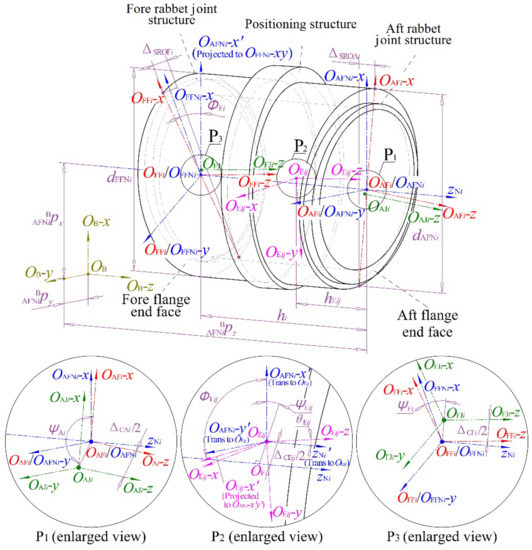
Figure 2.
Schematic of the rotor shape and position errors related to the assembly error.
The position and pose transmissions between the j-th positioning structure and the aft rabbet joint structure in the i-th rotor are derived using Equation (13).
where is the concentricity of the j-th positioning structure on the i-th rotor, represents the deviation direction of the positioning structure center, represents the distance between the positioning structure and the nominal aft flange end face, and and represent the transformed angle value and direction of the parallel error of the positioning structure axis, respectively.
The initial position and pose of the 1st rotor fixed on the fixture (separated from the six-axis mechanism) are derived using Equation (14). When the 1st rotor does not contain a rear rabbet joint structure, the coordinate origin of AJ1 is set at the center of the rear end face.
where is the column matrix that represents the nominal position of the aft end face of the 1st rotor relative to B, and represents its random initial position deviation; is the matrix of rolling, pitching, and yawing, which represents the random initial pose deflection of the 1st rotor.
3.2. Modeling of the Measurement Errors of Rotors
The transformation from the basic coordinate system B to the measurement coordinate system M is shown in Equation (15).
where the matrix elements represent the position of the measurement coordinate system; , and represent the triaxial angle errors.
The measuring objects include the position and pose of the last fixed rotor (i.e., ), the initial position and pose of the clamped rotor (i.e., ), and the position and pose of the positioning structure (i.e., ). There are two types of geometric features. One is the annular end face of the flange or positioning structure. Its normal vector is fitted to derive the pose column matrix , as shown in Equation (16). The other is the cylindrical face of the rabbet, the datum connection hole, or the positioning structure. The measured points are projected onto the corresponding datum end face. Subsequently, the cylindrical face center coordinates are fitted. The pose column matrices and , and the position column matrix are obtained.
The errors in the measuring processes are CMM mechanism errors, force deformation errors, thermal deformation errors, detection errors, etc. [60]. However, it is difficult to model these errors separately. Affected by a variety of system errors and random errors, the measured coordinates of each axis show a normal distribution with as the mathematical expectation μ, and as the standard deviation σ, as shown in Figure 3b. and represent the system errors and random errors in measurement errors, respectively. When in the triaxial directions are uniform, the spatial distribution of the possible locations of a measuring point is within the spherical range centered on the measuring point with only system error, as shown in Figure 3c. Generally, are easily pre-compensated in the CMM NC system by means of repetitive measurements and accuracy adjustments. Thus represents the comprehensive measurement accuracy of a CMM system.
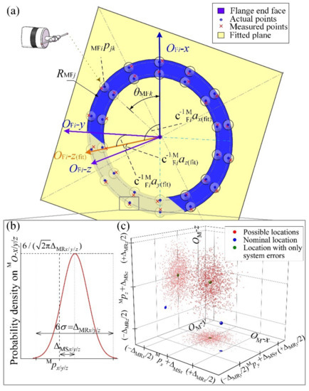
Figure 3.
Schematic of the measurement errors on the flange end face: (a) the actual flange end face and its fitted plane based on measured points; (b) normal distribution of measurement errors on each axis; and (c) spatial distribution of possible locations of the measuring point.
3.2.1. Measurement Errors on the Flange End Faces
Because the end face of the flange or positioning structure is annular, NMF measuring points are evenly distributed on J concentric circular paths, as shown in Figure 3a. The nominal coordinates of the k-th measuring point on the j-th circular path of the i-th rotor are derived using Equations (17) and (18).
where is the circumferential angle of and is the radius of the j-th circular path.
Under the influences of comprehensive measurement errors, the coordinates of the measured points are shown in Equations (19)–(21).
The fitted plane model with parameters a1, a2, and a3 is given by Equation (22).
The least-squares method can be used for plane fitting, that is, solving the minimum value of in Equation (23).
Because the angle between the coordinate axis OFi-z of the flange end face and the measurement coordinate axis OM-z is set to less than π/2, . Thereafter, the pose column matrix is obtained, as shown in Equations (24) and (25).
3.2.2. Measurement Errors on the Rabbet Joint Structures
When measuring the cylindrical face of the rabbet (or datum connection hole, positioning structure), NMJ measuring points are evenly distributed on the cylindrical face around its axis. Subsequently, the measured points are projected onto the fitted plane OFi-xy(fit). The center OJi (fit) is fitted, as shown in Figure 4.
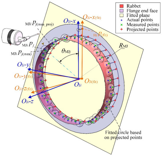
Figure 4.
Schematic of measurement errors on the rabbet joint structure.
The nominal coordinates of the j-th measuring point of the i-th rotor are derived using Equations (26) and (27).
where is the circumferential angle of , is the radius of the cylindrical face, and is the vertical distance between and end face.
Owing to the influences of measurement errors, the possible locations of the measuring points are within the normal distribution ranges of the triaxial coordinates of the points with only system errors. The projection coordinates of the measured points are given by Equation (31).
The fitted spatial circle on OFi-xy(fit) with parameters b1, b2, b3, and b4 is given by Equation (32).
The least-squares method can be used for fitting the center of the circle, that is, solving the minimum value of in Equation (33).
Similarly, the datum connection hole in the flange is measured, projected, and fitted. The coordinates of its center are . The pose column matrix is obtained as shown in Equations (34) and (35).
Therefore, the position and pose transformation matrix of the rabbet joint structure (or positioning structure), including the measurement errors, is given by Equation (36).
3.3. Modeling of the Six-Axis Mechanism Errors and Mounting Errors
A novel automated six-axis mechanism for rotor connection was designed and manufactured. The errors in the six-axis mechanism include manufacturing errors, assembly errors, NC errors, etc. [26] However, these large numbers of influencing factors are difficult to separately quantify. Thus, the mechanism error is attributed to the accumulation of the relative comprehensive position and pose errors of each two adjacent motion parts.
The modified D-H method with five parameters clarifies the relative position and pose with mechanism errors between the two adjacent parts. The D-H coordinate system is set at the joint of each motion execution part. The joint is used to connect with its upper part, as shown in Figure 5. The position and pose transformation of the upper part relative to the lower part is regarded as a combination of five consecutive rotations and translations: the D-H coordinate system rotates θ around the original axis O-z, translates d along the original axis O-z, translates a along the new axis O-z, rotates α around the new axis O-x, and then rotates around the new axis O-y. The transformation matrix from the lower to upper part is shown in Equation (37).
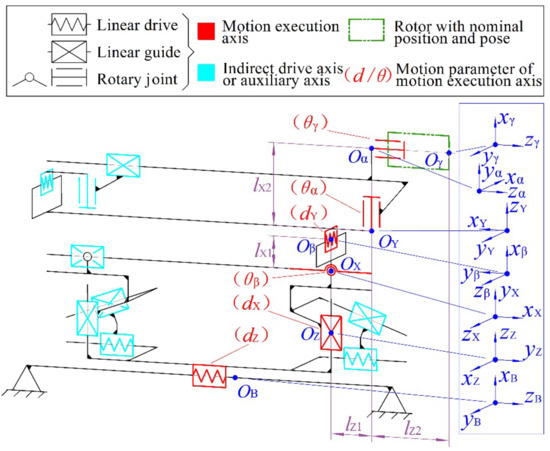
Figure 5.
Schematic of the D-H coordinate systems of the six motion execution parts.
The position and pose transmission in the six-axis mechanism is from the basic coordinate system B to the Z-axis part, X-axis part, β-axis part, Y-axis part, α-axis part, and finally to the γ-axis clamping fixture (i.e., the nominal position and pose of the aft rabbet joint structure of the clamped rotor). The transformation matrix is given by Equation (38).
The D-H parameters and their corresponding errors are listed in Table 1. dZ + ΔdZ, dX + ΔdX, θβ + δθβ, dY + ΔdY, θα + δθα, and θγ + δθγ represent motion variables with motion errors of the six axes. Motion errors are the main factors affecting the final comprehensive position and pose errors of the six-axis mechanism. Under the condition that the system errors are compensated through the NC system, the remaining random errors obey normal distributions. The deviation of each normal distribution is determined by the positioning accuracy of the corresponding axis. The other 24 errors are static errors representing the static relative position and pose among the axes, for example, δφβ and δφγ represent the parallel errors between the corresponding adjacent motion axes. These errors can be compensated through mechanism precision adjustment processes, or through the NC system.

Table 1.
Five D-H parameters with errors of the six-axis rotor connecting mechanism.
The mounting error of the (I + 1)-th rotor on the clamping fixture is indicated in Equation (39). The mounting error matrix is used in Equation (40) when solving the position and pose forward solution. On the premise of ignoring the measurement error, the acquisition method of the mounting error is as follows: move the six axes to their calibrated zero points where the mechanism errors have been corrected through precision adjustment, that is, . Subsequently, the initial position and pose of the clamped rotor are measured by the CMM to obtain . The mounting error is derived using Equation (41).
3.4. Modeling of the Rotor Final Assembly Errors
The assembly errors are defined by the relative positions and poses of the positioning structures on the different rotors, as shown in Figure 6.
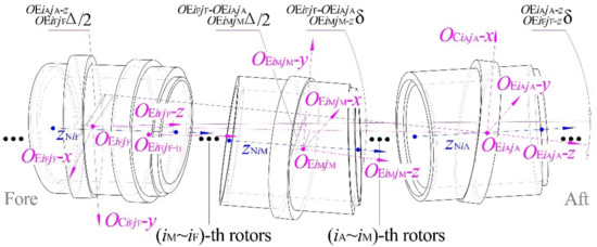
Figure 6.
Schematic of rotor assembly errors in the connecting processes.
If the measuring objects of the assembly error are located on the positioning structures of two rotors, the assembly position error of the iF-th positioning structure on the fore iF-th rotor relative to the iA-th positioning structure on the aft iA-th rotor is derived using Equations (42)–(44). The corresponding assembly pose error is derived using Equations (45) and (46).
If the measuring objects of assembly error are located on the positioning structures of three different rotors, that is, the original points of two positioning structures form a common reference line, the assembly position error of the iM-th positioning structure on the middle iM-th rotor relative to the common reference line OEiFiF-OEiAiA is derived using Equations (47)–(49). The corresponding assembly pose error is derived using Equations (50) and (51).
4. Construction and Application of the Rotor Assembly Error Prediction Algorithm
The Monte Carlo method is used to propose a rotor assembly error prediction algorithm based on the models of rotor shape and position errors, measurement errors, mechanism errors and mounting errors. In the prediction algorithm, the initial condition parameters, system errors, and random errors (sampled according to their related processes or mechanism accuracy) are input. Subsequently, multiple virtual rotor assemblies are simulated based on the actual connecting processes. Finally, the distributions of the assembly errors are output and analyzed.
4.1. Procedure of the Prediction Algorithm
The procedure for the rotor assembly accuracy prediction algorithm based on the Monte Carlo method is illustrated in Figure 7. In this procedure, N determines the total number of virtual assemblies under the same connecting conditions. An increase in N improves the prediction reliability while reducing the calculation efficiency. In each virtual assembly, the random initial position and pose of the 1st rotor are sampled, that is, and in Equation (14) are sampled to constitute . There are two methods to determine the shape and position errors of each rotor in Equations (12) and (13). In the first method, the distribution of each shape and position error is constructed according to the input rotor accuracy level, thereafter, the error value is sampled from its normal distribution, and the error direction angle is sampled from its uniform distribution. The other method is that all shape and position errors are directly input under the condition that they have been obtained through measurements.
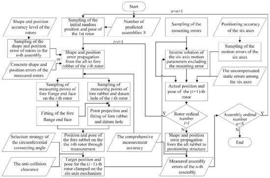
Figure 7.
Flow diagram of the rotor assembly error prediction algorithm considering multiple error sources.
The actual position and pose of the fore rabbet joint structure of the connected or fixed i-th rotor is determined by substituting Equations (12) and (14) into Equations (5) and (6). Subsequently, the virtual measuring points on the fore flange end face are generated using Equations (17)–(21), which are influenced by the CMM comprehensive measuring accuracy . The pose column matrix , representing the normal vector of the fore flange end face, is derived using Equations (23)–(25). The virtual projected points and of the measuring points on the fore rabbet joint structure and datum connection hole on the fitted plane OFFi-xy(fit) are generated using Equations (26)–(31). The position column matrix representing the fore rabbet joint structure center and the other two pose column matrices and are derived using Equations (33)–(35). The transformation matrix containing the measurement errors is obtained using Equations (15) and (36). The target matrix for the (i+1)-th rotor clamped on the six-axis mechanism is derived using Equation (8), where the connecting circumferential angle is calculated using its selection strategy.
The mounting error matrix for the (I + 1)-th rotor is derived using Equation (39). The matrix for generating the six-axis mechanism NC instruction excludes the effect of the mounting error. Thereafter, the motion variables dZ, dX, θβ, dY, θα, and θγ for controlling the six axes are obtained through inverse solutions from . Owing to the influence of static and motion errors in the six-axis mechanism, the actual position and pose is derived by substituting Table 1 into Equations (37) and (38). The random motion errors ΔdZ, ΔdX, δθβ, ΔdY, δθα, and δθγ are sampled from their normal distributions, which are related to the positioning accuracy of the six axes. The uncompensated items in the other 24 static errors are substituted into . Subsequently, the mounting error is substituted back into using Equation (40). Similarly, the actual position and pose of the (I + 2)-th rotor are derived through the above iterative calculations based on the determined of the (I + 1)-th rotor.
When the virtual connection of the n-th assembly containing I rotors is completed, the position and pose of the positioning structures, including their shape and position errors are derived by substituting and Equation (13) into Equation (2). Similarly, measurement errors are introduced again to fit the normal vector of the annular positioning faces and the centers of the cylindrical faces of the positioning structures through Equations (17)–(25) and Equations (26)–(33), respectively. The assembly errors are calculated by substituting into Equations (1) and (42)–(51). Thereafter, the virtual connection of the (n + 1)-th assembly is performed according to the above cyclic procedures. Finally, the assembly errors , , , and of the N assemblies are output for subsequent statistical analysis.
4.2. Inputs of the Prediction Algorithm
An aeroengine low-pressure turbine rotor simulator is applied, which has three rotors in an assembly. Considering the balance of prediction reliability and calculation efficiency, the total number N of virtual assemblies under the same connecting conditions is set to 100,000.
The initial position and pose of the 1st rotor are random in each virtual assembly. The corresponding matrix elements in obey uniform distributions, as shown in Equations (52) and (53). The matrix elements representing the datum positions are = 613.5, = 0, = 820 mm.
There are two methods to input the shape and position errors in each rotor. One is to sample the shape and position errors according to the designed tolerance and process capability of the parts. The process capability index CP is introduced into the prediction algorithm, which influences the distribution of the rotor shape and position error [61], as shown in Equation (54). The CP is set to 1.00, 1.33, and 1.67 (i.e., shape and position error qualification rates η = 99.73%, 99.9968%, and 99.999971%) respectively for presenting different accuracy levels of rotors. The standard deviation of the normal distributions of the rotor shape and position errors derived from their designed tolerance are listed in the second rows in Table 2, Table 3 and Table 4. In the prediction algorithm, assuming that the system errors in the shape and position errors of each rotor were corrected during the machining processes, the mathematical expectation is . The other matrix elements representing the error directions obey uniform distributions.
Table 2.
Designed standard deviations and measured concrete values of the shape and position errors of the 1st rotor (mm).
Table 3.
Designed standard deviations and measured concrete values of the shape and position errors of the 2nd rotor (mm).
Table 4.
Designed standard deviations and measured concrete values of the shape and position errors of the 3rd rotor (mm).
In the other input method, the measured values of the rotor shape and position errors are directly input into the corresponding matrices. The measured concrete errors of the three rotor assemblies used in the experiments are listed in the third to fifth rows in Table 2, Table 3 and Table 4.
The other matrix elements representing datum dimensions of the 1st rotor are dAN1 = Φ140, dFN1 = Φ237.4, hN1 = 151, and hE11 = 54 mm.
The other matrix elements representing datum dimensions of the 2nd rotor are dAN2 = Φ299.4, dFN2 = Φ308.7, hN2 = 11, and hE21 = −24 mm.
The other matrix elements representing datum dimensions of the 3rd rotor are: dFN3 = Φ308.7, hN2 = 11, hC31 = 68, and hC32 = 1037 mm.
According to the applied CMM, the comprehensive measuring accuracy = 0.002 mm. The measurement system errors because they are pre-compensated in the NC system. The matrix elements representing the location of the measurement coordinate system M are = 889.5, = −624, and = 67 mm. The number and nominal locations of the measuring points are listed in Table 5.
Table 5.
Number and distribution circle radius of the measuring points on different rotor structures.
The connecting circumferential angle is derived using the high- and low-point matching strategy which is commonly used in connecting processes, and it is also convenient for calculation in the prediction algorithm. The anti-collision clearance is set to 0.005 mm.
The static errors and motion system errors were reduced through the mechanism precision adjustment processes and the NC system, respectively. Hence, they are assumed to be zero in the prediction algorithm. The motion random errors are determined by the positioning accuracy of the drive axes and then converted to the corresponding motion execution axes. The motion error standard deviations σΔ obtained through the repeated measurement tests are listed in Table 6. The other D-H matrix elements representing the datum distance between the axes are lz1 = 107, lz2 = 206, lx1 = 97, and lx2 = 131 mm.
Table 6.
Standard deviations of the motion errors in the six-axis mechanism (mm).
The elements in the mounting error matrix in the prediction algorithm obey normal distributions, as shown in Equations (55) and (56). In the inverse and forward solutions of the six axes in the prediction algorithm, the measured mounting errors are excluded and introduced, respectively.
4.3. Results of the Prediction Algorithm
The distributions of the predicted six types of assembly errors under the conditions that the rotor CP = 1.00, 1.33, and 1.67 are shown in Figure 8. The rotor assembly errors are distributed with kurtosis and skewness . When CP improves from 1.00 to 1.33, and then to 1.67, the decline rates of the average value are 20.8% and 16.1%, respectively, the decline rates of are 22.8% and 18.9%, respectively, the decline rates of are 18.2% and 12.7% respectively, and the decline rates of are 17.8% and 12.9%, respectively. However, the decline rates of and are small. This is because the distance between the corresponding positioning structures is large (). The distance deviation between the center of the middle positioning structure and the long common reference line is insensitive to variations in rotor errors.
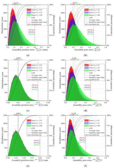
Figure 8.
Assembly error distributions of rotors under different shape and position accuracy levels: (a) assembly position error ; (b) assembly pose error ; (c) assembly position error ; (d) assembly pose error ; (e) assembly position error ; and (f) assembly pose error .
With regard to the rotor connection qualification rate, the qualification rate of each assembly error is higher than 93%. The connection qualified condition of a rotor assembly is that all six errors are lower than their qualified upper limits. The final connection qualification rates of the rotor assemblies are 88.9%, 97.4%, and 99.3% when CP = 1.00, 1.33, and 1.67, respectively. It can be seen that even if the rotors have relatively low shape and position accuracy (CP = 1.00), the connection qualification rate is still significantly higher than that less than 50% when using traditional manual connection processes. If the rotors have general or high accuracy (CP ≥ 1.33), the connection qualification rate is higher than 97%. In general, the prediction results show that the novel mechanical system (three-axis CMM, six-axis rotor connecting mechanism, and clamping fixture) has high applicability for rotors with different accuracies.
5. Verification Experiment
To verify the proposed prediction method, three different rotors satisfying the shape and position accuracy requirements (CP ≥ 1.00) are applied in the connection experiments. The rotor shape and position errors are presented in Table 2, Table 3 and Table 4. The motion errors of the pre-compensated six-axis mechanism are listed in Table 6. The comprehensive measuring accuracy of the applied three-axis CMM equipped with a contact probe (RENISHAW OMP40-2) is = 0.002 mm. The number of connection experiments for each rotor assembly is 30.
The experimental setup is illustrated in Figure 9. The experimental process of each assembly is consistent with the prediction algorithm flow, which includes the following steps: Step 1: the 1st rotor is mounted on the aft adjustable fixture separated from the six-axis mechanism. The initial position and pose are adjusted randomly according to Equations (52) and (53) using the adjustable fixture. Step 2: the 2nd rotor is mounted on the clamping fixture on the six-axis mechanism. Thereafter, the six axes move to their calibrated zero points, where the mechanism errors were corrected through precision adjustment. The current position and pose of the 2nd rotor are measured by the CMM to obtain the . The mounting error is derived using Equation (41). Step 3: the initial position and pose of the fore rabbet joint structure of the 1st rotor are measured using the parameters in Table 5, and is fitted using Equations (22)–(25) and (31)–(36). Step 4: the target matrix for the 2nd rotor is obtained using Equation (8) with derived using the high- and low-point matching strategy, and anti-collision clearance = 0.005 mm. To exclude mounting errors, the motion parameters of the six axes are solved inversely according to . Subsequently, the NC instructions of the six axes are generated to adjust the position and pose of the 2nd rotor, and connect it to the 1st rotor. Local gaskets and a few bolts are used to fasten the two rotors to minimize the impact of fastening on the assembly errors. Step 5: repeat Steps 2-4 for the connection of the 3rd rotor. Step 6: the position and pose matrices , , and of the four positioning structures are obtained according to the measuring and fitting methods similar to Step 3. The assembly errors are then derived using Equations (1), (15) and (42)–(51).
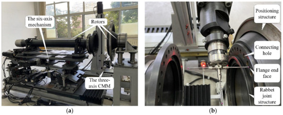
Figure 9.
Experimental setup: (a) the six-axis rotor connecting mechanism and three-axis CMM; and (b) measuring process.
The experimental results are shown in Figure 10. The measured shape and position errors of the rotors in the three assemblies are also input into the prediction algorithm for comparison. It can be seen that the distribution ranges of the six assembly errors obtained from 30 experiments of each assembly are within the corresponding min-max ranges of 100,000 predicted results. Compared with the corresponding average values of the six assembly errors of each assembly in the predictions, the deviation rates of the corresponding experimental results are all lower than 14%.
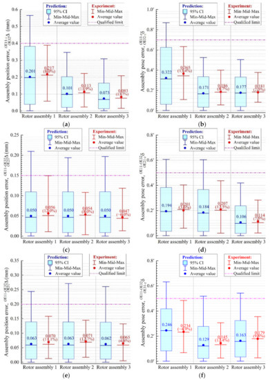
Figure 10.
Comparisons between the assembly error results in predictions and experiments: (a) assembly position error ; (b) assembly pose error ; (c) assembly position error ; (d) assembly pose error ; (e) assembly position error ; and (f) assembly pose error .
There are still small deviations between the distribution ranges of the experimental assembly errors and the 95% confidence intervals (CIs) of the corresponding predicted results. The deviations may be caused by the following factors: (1) In the characterization model for rotor shape and position errors, the flange SRO is based on a typical geometric feature with a single high point caused by turning or milling processes. This is not applicable to specially processed rotors with multiple high points; (2) The system errors among the six axes of the rotor connecting mechanism are pre-compensated through the mechanism precision adjustment processes and NC system. However, there may be non-zero values that are not input into the mechanism error model because of the mutual interference of a large number of errors; (3) The system errors in the three-axis CMM are not completely compensated. The fitting methods have fitting errors; (4) The effect of the force is not considered in the prediction method, for example, the connection contact force, fastening force, and gravity. In general, the proposed prediction method considers the influences of the main error sources and is highly consistent with the actual connection processes. The deviations between the predicted assembly errors and corresponding experimental results are acceptable. The proposed rotor assembly error prediction method has high accuracy and practical significance.
6. Conclusions
To propose a rotor assembly error prediction method under the influence of multiple error sources based on the use of a novel multi-axis measuring and connecting mechanism, mathematical models and propagation algorithm of multiple types of errors are established. Models for indicating the rotor shape and position errors, measurement errors, six-axis rotor connecting mechanism errors, mounting errors, and rotor assembly errors are established mainly based on homogeneous coordinate transformation matrices and differential matrices. A new prediction algorithm for the rotor assembly error considering the abovementioned error sources is proposed, which is highly consistent with actual connecting processes. Subsequently, experiments are conducted to verify the prediction method. The following conclusions are drawn:
- (1)
- The kurtosis and skewness of the distributions of all predicted assembly errors are positive. When the rotor process capability index CP is set to 1.00, 1.33, and 1.67, respectively, the average values of the assembly position errors are = 0.149, 0.118, and 0.099 mm; = 0.051, 0.050, and 0.049 mm; and = 0.064, 0.063, and 0.062 mm, respectively; the average values of assembly pose errors are = 0.294′, 0.227′, and 0.184′; = 0.203′, 0.166′, and 0.145′; and = 0.236′, 0.194′, and 0.169′, respectively. Detailed statistical results are obtained using the proposed prediction method;
- (2)
- If CP improves from 1.00 to 1.33, and then to 1.67, the decline rates of , ,, and range from 12.0% to 23.0%, while the decline rates of and are small. The last two assembly position errors are insensitive to changes in rotor shape and position errors, because they take a long-distance common line as reference. In general, the improvement in the rotor shape and position accuracy reduces most assembly errors to varying degrees;
- (3)
- The connection qualification rate is higher than 97% when the rotors have general or high shape and position accuracy (i.e., CP ≥ 1.33). Even if the rotors have relatively low accuracy (i.e., CP = 1.00), the connection qualification rate achieves 88.9%. It is significantly higher than the qualification rate of less than 50% when using the traditional manual connection processes. According to the predictions, the new mechanical system (three-axis CMM, the six-axis rotor connecting mechanism, and clamping fixture) has high applicability for rotors with different accuracy levels;
- (4)
- Predictions and experiments based on three aeroengine rotor assemblies show that: The min-max ranges of the six assembly errors obtained from 30 experiments for each assembly are within those of the corresponding 100,000 predicted results. The deviation rates of the corresponding experimental average values of the six assembly errors relative to those of the predictions are all lower than 14%. The proposed prediction method has acceptable accuracy and practical significance.
Author Contributions
Conceptualization, T.Z.; methodology, T.Z. and H.G.; software, T.Z. and L.L.; validation, T.Z.; formal analysis, T.Z.; investigation, T.Z.; resources, T.Z. and X.W.; data curation, T.Z., L.L., J.C. and C.P.; writing—original draft preparation, T.Z.; writing—review and editing, X.W., L.L., J.C. and C.P.; visualization, T.Z.; supervision, H.G.; project administration, H.G. All authors have read and agreed to the published version of the manuscript.
Funding
This work is supported by the National Natural Science Foundation of China (U1908232); the National Development Plan (2019YFA0705304); and the Fundamental Research Funds for the Central Universities (82231073).
Institutional Review Board Statement
Not applicable.
Informed Consent Statement
Not applicable.
Data Availability Statement
Not applicable.
Conflicts of Interest
The authors declare no conflict of interest.
Nomenclature
| AFi/FFi | Aft/fore flange end face on the i-th rotor |
| AFNi/FFNi | Nominal aft/fore flange end face without any shape or position errors on the i-th rotor |
| AJi/FJi | Aft/fore rabbet joint structure on the i-th rotor |
| AN1 | Aft nominal end face on the 1st rotor |
| a1/2/3 | Fitting parameter of annular end face |
| B | Basic coordinate system |
| b1/2/3/4 | Fitting parameter of the cylindrical face |
| Process capability index | |
| Error transformation matrix from A to B | |
| Nominal diameter of aft/fore flange end face on the i-th rotor (mm) | |
| Differential matrix of | |
| Eij | The j-th positioning structure on the i-th rotor |
| Distance between the j-th positioning structure and nominal aft flange end face on the i-th rotor (mm) | |
| Actual/nominal distance between fore and aft flange end faces on the i-th rotor (mm) | |
| M | Measuring coordinate system |
| N | Total number of virtual assemblies under the same connecting condition |
| Position column matrix in | |
| Element in position column matrix | |
| NMF/MJ | Number of points for measuring annular end face/cylindrical face |
| First/second/third pose column matrix in excluding last element 0 | |
| The k-th nominal point on the j-th circular path for measuring annular end face of the i-th rotor | |
| The j-th nominal point for measuring cylindrical face of the i-th rotor | |
| / | Measured point/Projection of measured point |
| Radius of the j-th circular path for measuring annular end face (mm) | |
| Radius of the cylindrical face (mm) | |
| Rotation transformation matrix | |
| Matrix of rolling, pitching, and yawing | |
| Transformation matrix from A to B (A/B is the reference/current coordinate system) | |
| Obtained transformation matrix after measurement and fitting | |
| Target matrix for generating NC instructions | |
| Transformation matrix when six axes are at their calibrated zero points | |
| Translation transformation matrix | |
| Rotor shape and position tolerance | |
| Anti-collision clearance (mm) | |
| Concentricity of aft/fore rabbet joint structure of the i-th rotor (mm) | |
| Concentricity of the j-th positioning structure on the i-th rotor (mm) | |
| Comprehensive measuring accuracy of CMM system (mm) | |
| Aft/fore flange end face run-out of the i-th rotor (mm) | |
| / | Assembly position/pose error of iF-th positioning structure on fore iF-th rotor relative to iA-th positioning structure on aft iA-th rotor |
| / | Assembly position/pose error of iM-th positioning structure on middle iM-th rotor relative to common reference line OEiFiF-OEiAiA |
| / | Linear/rotational motion error in six-axis mechanism |
| Transformed angle value representing parallel error of axis of j-th positioning structure on i-th rotor (′) | |
| D-H parameters of six-axis mechanism | |
| Circumferential angle of / (rad) | |
| Standard deviation of rotor shape and position error | |
| Standard deviation of motion error of six-axis mechanism | |
| Deflection angle of rolling/pitching/yawing of the 1st rotor (rad) | |
| Deflection direction of axis of the j-th positioning structure on the i-th rotor caused by parallel error (rad) | |
| Circumferential angle between high points of fore and aft flange end faces on i-th rotor (rad) | |
| Connecting circumferential angle between the i-th and (i+1)-th rotors (rad) | |
| Direction of aft/fore rabbet center deviation of the i-th rotor (rad) | |
| Direction of center deviation of the j-th positioning structure on the i-th rotor (rad) |
References
- Sun, C.; Hu, M.; Liu, Y.; Zhang, M.; Liu, Z.; Chen, D.; Tan, J. A method to control the amount of unbalance propagation in precise cylindrical components assembly. Proc. Inst. Mech. Eng. B J. Eng. Manuf. 2019, 233, 2458–2468. [Google Scholar] [CrossRef]
- Liu, A.; Ju, Y.; Zhang, C. Parallel rotor/stator interaction methods and steady/unsteady flow simulations of multi-row axial compressors. Aerosp. Sci. Technol. 2021, 116, 106859. [Google Scholar] [CrossRef]
- Jin, S.; Ding, S.; Li, Z.; Yang, F.; Ma, X. Point-based solution using Jacobian-Torsor theory into partial parallel chains for revolving components assembly. J. Manuf. Syst. 2018, 46, 46–58. [Google Scholar] [CrossRef]
- Zhu, Y.; Huang, X.; Fang, W.; Li, S. Trajectory Planning Algorithm Based on Quaternion for 6-DOF Aircraft Wing Automatic Position and Pose Adjustment Method. Chin. J. Aeronaut. 2010, 23, 707–714. [Google Scholar]
- Lee, N.K.S.; Yu, G.; Joneja, A.; Ceglarek, D. The modeling and analysis of a butting assembly in the presence of workpiece surface roughness and part dimensional error. Int. J. Adv. Manuf. Technol. 2006, 31, 528–538. [Google Scholar] [CrossRef]
- Sun, H.; Wang, J.; Chen, K.; Xia, H.; Feng, X.; Chang, Z. A tip clearance prediction model for multistage rotors and stators in aero-engines. Chin. J. Aeronaut. 2021, 34, 343–357. [Google Scholar] [CrossRef]
- Liu, J.; Jin, J.; Shi, J. State Space Modeling for 3-D Variation Propagation in Rigid-Body Multistage Assembly Processes. IEEE Trans. Autom. Sci. Eng. 2010, 7, 274–290. [Google Scholar]
- Zhang, Z.; Zhang, Z.; Jin, X.; Zhang, Q. A novel modelling method of geometric errors for precision assembly. Int. J. Adv. Manuf. Technol. 2017, 94, 1139–1160. [Google Scholar] [CrossRef]
- Bakker, O.J.; Popov, A.A.; Ratchev, S.M. Variation analysis of automated wing box assembly. Procedia CIRP 2017, 63, 406–411. [Google Scholar] [CrossRef]
- Peng, Y.; Hao, L.; Huang, X.; Li, S. A pre-assembly analysis technology of aircraft components based on measured data. Meas. Sci. Technol. 2022, 33, 075005. [Google Scholar] [CrossRef]
- Sun, C.; Li, C.; Liu, Y.; Liu, Z.; Wang, X.; Tan, J. Prediction Method of Concentricity and Perpendicularity of Aero Engine Mul-tistage Rotors Based on PSO-BP Neural Network. IEEE Access 2019, 7, 132271–132278. [Google Scholar] [CrossRef]
- Ding, S.; Jin, S.; Li, Z.; Chen, H. Multistage rotational optimization using unified Jacobian-Torsor model in aero-engine assembly. Proc. Inst. Mech. Eng. B J. Eng. Manuf. 2019, 233, 251–266. [Google Scholar] [CrossRef]
- Zhang, T.; Zhang, Z.; Jin, X.; Ye, X.; Zhang, Z. An innovative method of modeling plane geometric form errors for precision assembly. Proc. Inst. Mech. Eng. B J. Eng. Manuf. 2016, 230, 1087–1096. [Google Scholar] [CrossRef]
- Sun, Q.; Zhao, B.; Liu, X.; Mu, X.; Zhang, Y. Assembling deviation estimation based on the real mating status of assembly. Comput. Aided Des. 2019, 115, 244–255. [Google Scholar] [CrossRef]
- Sun, C.; Liu, Z.; Liu, Y.; Wang, X.; Tan, J. An Adjustment Method of Geometry and Mass Centers for Precision Rotors Assembly. IEEE Access 2019, 7, 169992–170002. [Google Scholar] [CrossRef]
- Mu, X.; Wang, Y.; Yuan, B.; Sun, W.; Liu, C.; Sun, Q. A New assembly precision prediction method of aeroengine high-pressure rotor system considering manufacturing error and deformation of parts. J. Manuf. Syst. 2021, 61, 112–124. [Google Scholar] [CrossRef]
- Lowth, S.; Axinte, D.A. An assessment of “variation conscious” precision fixturing methodologies for the control of circularity within large multi-segment annular assemblies. Precis. Eng. 2014, 38, 379–390. [Google Scholar] [CrossRef][Green Version]
- Sun, C.; Wang, B.; Liu, Y.; Wang, X.; Li, C.; Wang, H.; Tan, J. Design of high accuracy cylindrical profile measurement model for low-pressure turbine shaft of aero engine. Aerosp. Sci. Technol. 2019, 95, 105442. [Google Scholar] [CrossRef]
- Wang, J.; Sun, Q.; Yuan, B. Novel on-machine measurement system and method for flatness of large annular plane. Meas. Sci. Technol. 2020, 31, 015004. [Google Scholar] [CrossRef]
- Yu, L.; Zhang, Y.; Bi, Q.; Wang, Y. Research on surface normal measurement and adjustment in aircraft assembly. Precis. Eng. 2017, 50, 482–493. [Google Scholar] [CrossRef]
- Jamshidi, J.; Kayani, A.; Iravani, P.; Maropoulos, P.G.; Summers, M.D. Manufacturing and assembly automation by integrated metrology systems for aircraft wing fabrication. Proc. Inst. Mech. Eng. B J. Eng. Manuf. 2010, 224, 25–36. [Google Scholar] [CrossRef]
- Díaz-Tena, E.; Ugalde, U.; de Lacalle, L.N.L.; de la Iglesia, A.; Calleja, A.; Campa, F.J. Propagation of assembly errors in multitasking machines by the homogenous matrix method. Int. J. Adv. Manuf. Technol. 2013, 68, 149–164. [Google Scholar] [CrossRef]
- Lin, P.D.; Tzeng, C.S. Modeling and measurement of active parameters and workpiece home position of a multi-axis machine tool. Int. J. Mach. Tools Manuf. 2008, 48, 338–349. [Google Scholar] [CrossRef]
- Lei, P.; Zheng, L. An automated in-situ alignment approach for finish machining assembly interfaces of large-scale com-ponents. Robot. Comput. Int. Manuf. 2017, 46, 130–143. [Google Scholar] [CrossRef]
- Papastathis, T.; Ryll, M.; Bone, S.; Ratchev, S. Development of a Reconfigurable Fixture for the Automated Assembly and Disassembly of High Pressure Rotors for Rolls-Royce Aero Engines. In Precision Assembly Technologies and Systems. IPAS 2010; Ratchev, S., Ed.; IFIP Advances in Information and Communication Technology; Springer: Berlin/Heidelberg, Germany, 2010; Volume 315, pp. 283–289. [Google Scholar] [CrossRef]
- Ramesh, R.; Mannan, M.A.; Poo, A.N. Error compensation in machine tools—A review Part I: Geometric, cutting-force induced and fixture-dependent errors. Int. J. Mach. Tools Manuf. 2000, 40, 1235–1256. [Google Scholar] [CrossRef]
- Chen, Z.; Du, F.; Tang, X. Position and orientation best-fitting based on deterministic theory during large scale assembly. J. Intell. Manuf. 2018, 29, 827–837. [Google Scholar] [CrossRef]
- Yang, Z.; Hussain, T.; Popov, A.A.; McWilliam, S. Novel Optimization Technique for Variation Propagation Control in An Aero-Engine Assembly. Proc. Inst. Mech. Eng. B J. Eng. Manuf. 2011, 225, 100–111. [Google Scholar] [CrossRef]
- Yang, H.; Tsai, P. Mathematical model of S-shaped gear surface. J. Mech. Sci. Technol. 2021, 35, 2841–2850. [Google Scholar] [CrossRef]
- Li, Y.; Zhang, L.; Wang, Y. An optimal method of posture adjustment in aircraft fuselage joining assembly with engineering constraints. Chin. J. Aeronaut. 2017, 30, 2016–2023. [Google Scholar] [CrossRef]
- Whitney, D.E.; Gilbert, O.L.; Jastrzebski, M. Representation of geometric variations using matrix transforms for statistical tolerance analysis in assemblies. Res. Eng. Des. 1994, 6, 191–210. [Google Scholar] [CrossRef]
- Wu, Y.; Chen, C. An automatic generation method of the coordinate system for automatic assembly tolerance analysis. Int. J. Adv. Manuf. Technol. 2018, 95, 889–903. [Google Scholar] [CrossRef]
- Zhang, M.; Liu, Y.; Sun, C.; Wang, X.; Tan, J. Measurements error propagation and its sensitivity analysis in the aero-engine multistage rotor assembling process. Rev. Sci. Instrum. 2019, 90, 115003. [Google Scholar] [CrossRef] [PubMed]
- Zhou, Z.; Liu, W.; Wu, Q.; Wang, Y.; Yu, B.; Yue, Y.; Zhang, J. A Combined Measurement Method for Large-Size Aerospace Components. Sensors 2020, 20, 4843. [Google Scholar] [CrossRef] [PubMed]
- Iwasa, T.; Harada, T. A Precise Connection Method for Surface Shape Data Measured by the Grating Projection Method. Trans. Jpn. Soc. Aeronaut. Space Sci. 2016, 59, 251–257. [Google Scholar] [CrossRef][Green Version]
- Ahn, H.K.; Kang, H.; Ghim, Y.; Yang, H. Touch Probe Tip Compensation Using a Novel Transformation Algorithm for Co-ordinate Measurements of Curved Surfaces. Int. J. Precis. Eng. Man. 2019, 20, 193–199. [Google Scholar] [CrossRef]
- Deng, Z.; Li, S.; Huang, X. A flexible and cost-effective compensation method for leveling using large-scale coordinate measuring machines and its application in aircraft digital assembly. Meas. Sci. Technol. 2018, 29, 065904. [Google Scholar] [CrossRef]
- Calvo, R. Sphericity measurement through a new minimum zone algorithm with error compensation of point coordinates. Measurement 2019, 138, 291–304. [Google Scholar] [CrossRef]
- Hu, Q.; Zhang, D.; Wu, Z. Trajectory planning and tracking control for 6-DOF Stanford manipulator based on adaptive sliding mode multi-stage switching control. Int. J. Robust Nonlinear Control 2021, 31, 6602–6625. [Google Scholar] [CrossRef]
- Cai, L.; Zhang, Z.; Cheng, Q.; Liu, Z.; Gu, P.; Qi, Y. An approach to optimize the machining accuracy retainability of multi-axis NC machine tool based on robust design. Precis. Eng. 2016, 43, 370–386. [Google Scholar] [CrossRef]
- Zhou, W.; Chen, W.; Liu, H.; Li, X. A new forward kinematic algorithm for a general Stewart platform. Mech. Mach. Theory 2015, 87, 177–190. [Google Scholar] [CrossRef]
- Yang, J.; Ding, H. A new position independent geometric errors identification model of five-axis serial machine tools based on differential motion matrices. Int. J. Mach. Tools Manuf. 2016, 104, 68–77. [Google Scholar] [CrossRef]
- Guo, J.; Li, B.; Liu, Z.; Hong, J.; Zhou, Q. A new solution to the measurement process planning for machine tool assembly based on Kalman filter. Precis. Eng. 2016, 43, 356–369. [Google Scholar] [CrossRef]
- Chen, J.-X.; Lin, S.-W.; Zhou, X.-L. A comprehensive error analysis method for the geometric error of multi-axis machine tool. Int. J. Mach. Tools Manuf. 2016, 106, 56–66. [Google Scholar] [CrossRef]
- Tang, W.; Li, Y.; Yu, J.; Zhang, J.; Yu, L. Locating error analysis for workpieces with general fixture layouts and parameterized tolerances. Proc. Inst. Mech. Eng. B J. Eng. Manuf. 2016, 230, 416–427. [Google Scholar] [CrossRef]
- Fallah, M.; Arezoo, B. Modelling and compensation of fixture locators’ error in CNC milling. Int. J. Prod. Res. 2013, 51, 4539–4555. [Google Scholar] [CrossRef]
- Vallance, R.R.; Morgan, C.; Slocum, A.H. Precisely positioning pallets in multi-station assembly systems. Precis. Eng. 2004, 28, 218–231. [Google Scholar] [CrossRef]
- Wei, P.; Lu, Z.; Song, J. Extended Monte Carlo Simulation for Parametric Global Sensitivity Analysis and Optimization. AIAA J. 2014, 52, 867–878. [Google Scholar] [CrossRef]
- Wu, F.; Cao, X.; Butcher, E.A.; Wang, F. Dynamics and control of spacecraft with a large misaligned rotational component. Aerosp. Sci. Technol. 2019, 87, 207–217. [Google Scholar] [CrossRef]
- Wen, X.; Zhao, Y.; Wang, D.; Pan, J. Adaptive Monte Carlo and GUM methods for the evaluation of measurement uncertainty of cylindricity error. Precis. Eng. 2013, 37, 856–864. [Google Scholar] [CrossRef]
- Schwenke, H.; Knapp, W.; Haitjema, H.; Weckenmann, A.; Schmitt, R.; Delbressine, F. Geometric error measurement and compensation of machines—An update. CIRP Ann. 2008, 57, 660–675. [Google Scholar] [CrossRef]
- Cui, G.; Lu, Y.; Li, J.; Gao, D.; Yao, Y. Geometric error compensation software system for CNC machine tools based on NC program reconstructing. Int. J. Adv. Manuf. Technol. 2012, 63, 169–180. [Google Scholar] [CrossRef]
- Guo, C.; Liu, J.; Jiang, K. Efficient statistical analysis of geometric tolerances using unified error distribution and an analytical variation model. Int. J. Adv. Manuf. Technol. 2016, 84, 347–360. [Google Scholar]
- Yang, Z.; McWilliam, S.; Popov, A.A.; Hussain, T. A probabilistic approach to variation propagation control for straight build in mechanical assembly. Int. J. Adv. Manuf. Technol. 2013, 64, 1029–1047. [Google Scholar] [CrossRef]
- Wang, Q.; Huang, P.; Li, J.; Ke, Y. Uncertainty evaluation and optimization of INS installation measurement using Monte Carlo Method. Assem. Autom. 2015, 35, 221–233. [Google Scholar] [CrossRef]
- Cui, Z.; Du, F. Assessment of large-scale assembly coordination based on pose feasible space. Int. J. Adv. Manuf. Technol. 2019, 104, 4465–4474. [Google Scholar] [CrossRef]
- Tang, H.; Li, C.; Zhang, Z.; Ko, T.J. A novel geometric error modeling optimization approach based on error sensitivity analysis for multi-axis precise motion system. J. Mech. Sci. Technol. 2019, 33, 3435–3444. [Google Scholar] [CrossRef]
- Liu, Y.; Yuan, M.; Cao, J.; Cui, J.; Tan, J. Evaluation of measurement uncertainty in H-drive stage during high acceleration based on Monte Carlo method. Int. J. Mach. Tools Manuf. 2015, 93, 1–9. [Google Scholar] [CrossRef]
- Liu, Y.; Zhang, M.; Sun, C.; Hu, M.; Chen, D.; Liu, Z.; Tan, J. A method to minimize stage-by-stage initial unbalance in the aero engine assembly of multistage rotors. Aerosp. Sci. Technol. 2019, 85, 270–276. [Google Scholar] [CrossRef]
- Fruciano, C. Measurement error in geometric morphometrics. Dev. Genes Evol. 2016, 226, 139–158. [Google Scholar] [CrossRef]
- Chao, M.T.; Lin, D. Another look at the process capability index. Qual. Reliab. Eng. Int. 2006, 22, 153–163. [Google Scholar] [CrossRef]


Publisher’s Note: MDPI stays neutral with regard to jurisdictional claims in published maps and institutional affiliations. |
© 2022 by the authors. Licensee MDPI, Basel, Switzerland. This article is an open access article distributed under the terms and conditions of the Creative Commons Attribution (CC BY) license (https://creativecommons.org/licenses/by/4.0/).