Rendering Natural Bokeh Effects Based on Depth Estimation to Improve the Aesthetic Ability of Machine Vision

Abstract

Machine vision is the key to realizing computer-vision tasks such as human–computer interaction and autonomous driving. However, human perception of an image’s beauty is innate. If a machine can increase aesthetic awareness, it will greatly improve the comfort of human perception in human–computer interaction. The bokeh effect is one of the most important ways to improve the artistic beauty of photographic images and the image aesthetic quality. Bokeh rendering of an image can highlight the main object of the image and blur unnecessary or unattractive background details. The existing methods usually have unrealistic rendering effects with obvious artifacts around the foreground boundary. Therefore, we propose a natural bokeh-rendering method based on depth estimation that satisfies the following characteristics: objects in the focal plane are clear and out-of-focus objects are blurred; and the further away from the focal plane, the more blurred the objects are. Our method consists of three modules: depth estimation, background subdivision, and bokeh rendering. The background-subdivision module can select different focal planes to obtain different blur radii, making the bokeh-rendering effect more diverse, so that it does not oversegment objects. The bokeh-rendering module adjusts the degree of bokeh by adjusting the blur-radius factor. In the experimental section, we analyze the model results and present the visualization results.

1. Introduction

In this era where everyone is a photographer, we can shoot the scenery, food, and people we like at any time. Aesthetics is an innate ability of human beings. Now we are not only satisfied with photos that can record moments, but also hope to shoot more beautiful scenery. However, the ability of machines to image aesthetics needs to be learned. If a machine can have the human perception of beauty, then in computer-vision tasks such as human–computer interaction [1], automatic driving [2], and detection [3], humans can have a better feeling. For humans, image processing such as image enhancement, image recoloring, image denoising, and bokeh-effect rendering are important methods to improve the aesthetic quality of images [4]. This article focuses on bokeh-effect rendering.

Bokeh-effect rendering was originally used for portraits, blurring the background to make the person stand out. Initially, most researchers used the method [5] of image segmentation to segment the foreground and background, and achieve the bokeh effect by blurring the background. However, such methods do not take into account the distance of the object from the camera. The acquisition of the bokeh-effect image is that the cameraman adjusts the camera lens so that the object at a certain distance from the camera can be clearly imaged; that is, objects within a certain distance before and after the focal plane are clearly photographed, and objects at other distances are in a blurred state, and the farther away from the focal plane, the more blurred the objects are.

Therefore, if we want to render a natural camera bokeh effect, we need to know the depth information of the objects in the image. At present, many depth cameras can obtain depth information of images while taking pictures. Such cameras can be roughly divided into three categories: binocular stereo vision, structured light, and time-of-flight. The image captured by the depth camera contains depth information, but the image captured by the ordinary camera does not. When rendering a normal image with the bokeh effect, we need to first estimate the depth of the image.

In order to make the bokeh effect more in line with the effect captured by a natural camera, we use the depth information to achieve it. In this paper, we propose a single-image bokeh-effect-rendering method based on depth information. Our main innovations are as follows:

(1)

It is difficult to obtain image-depth data, but the model does not perform well when the training data are limited. Therefore, we use the idea of style transfer to synthesize images and increase the number of datasets.

(2)

In order to better combine the relationship between image parts, we propose an image-depth-estimation model based on Transformer.

(3)

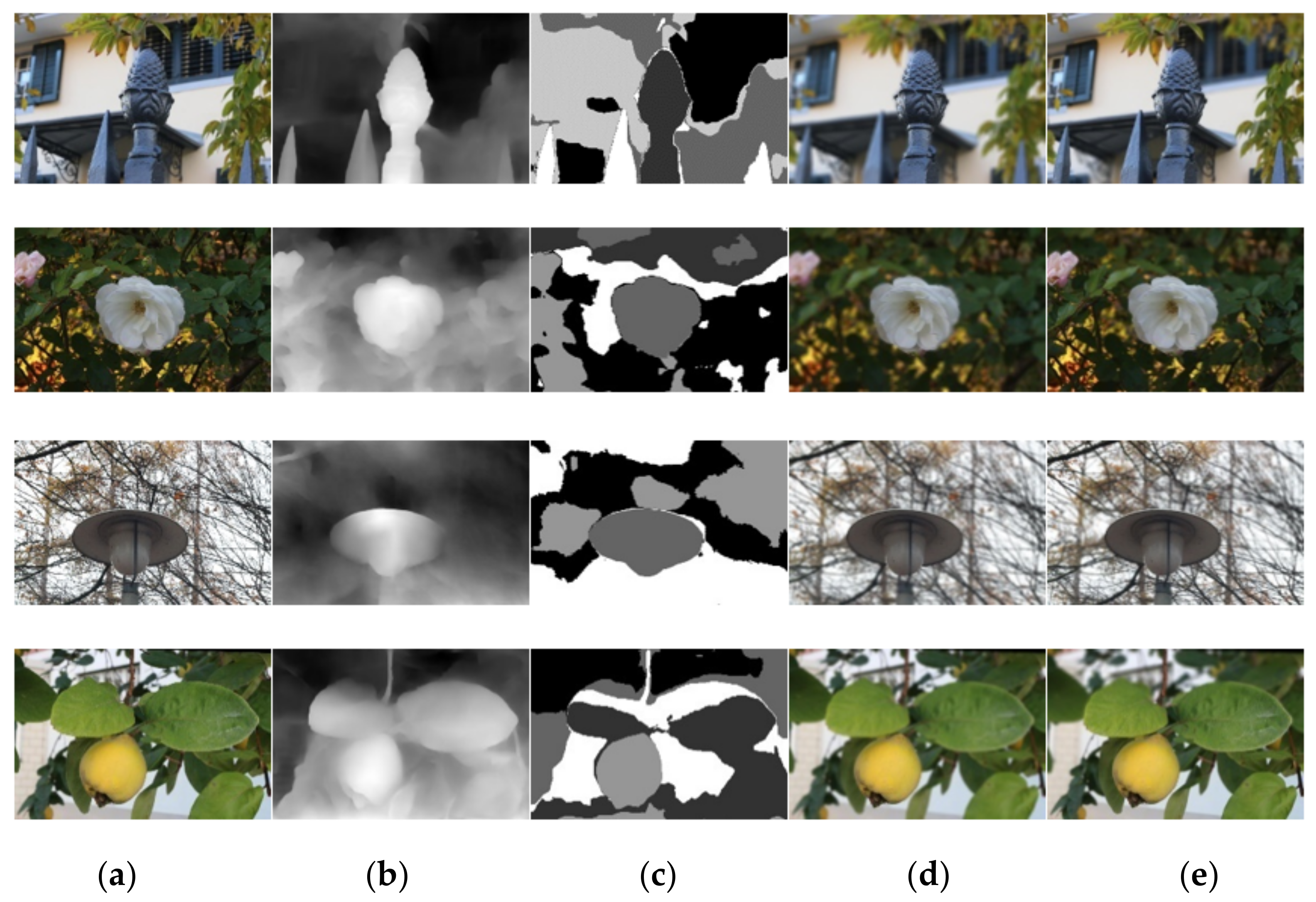
In order to meet the characteristics of the bokeh image—the further the object is from the focal plane, the more blurred it is—we propose the image-background subregion-blurring method. Different blur radii can be obtained by choosing different focal planes, which makes the bokeh-rendering effect more diverse and does not oversegment the objects, producing bokeh images with different effects.

2. Related Work

2.1. Image-Depth Estimation Based on Deep Learning

The Convolutional Neural Network (CNN) was first used in the field of image-depth estimation by EIGEN et al. [6] in 2014. Compared to traditional methods, deep-learning methods have higher accuracy in small occlusions, large occlusions, and even in the absence of ground truth. In the following paper, we will categorize the different network structures in terms of supervised and unsupervised learning and review the advantages and disadvantages of different approaches.

Most CNN-based methods for image-depth estimation use multibranch parallel and recursive skip-connected CNN network structures. In addition, many models add attention modules or use multiple loss functions. The diagram of the model is shown in Figure 1. The model proposed by EIGEN et al. in 2014 used two networks in parallel and then fused, which was improved to three branches in parallel in 2015 [7]. The network proposed by Li et al. [8] in 2017 used VGG [9] to form three branches and added skip connections, and proposed a correlated image-level loss function with a regular term, which makes better use of the augmented data, enhances the network generalization, and improves the estimation accuracy. The method proposed by Kim [10] et al. in 2018 used a parallel structure of two branches, where one branch dealt with the whole image to learn global features and one branch dealt with the image block to learn local features. In 2018 Zhang [11] et al. proposed a recursive hard-mining network (PHN), which uses a recursive skip-connected structure, along with a hard-mining loss function focusing on locations where depth is difficult to predict, added at multiple locations of the network. In 2021 Chen et al. proposed an ACAN [12] network with a multibranch parallel structure and added content-attention module. The idea of the GAN-based image-depth estimation method is that the generator generates a depth map and the discriminator determines whether the depth map is true or false. For example, in the method proposed by Islam [13] et al. in 2021, for the input image and the depth map pair, the generator generates two fake depth maps, and then the discriminator determines which of the three depth maps is the true image pair with the input image.

Figure 1. Diagram of the supervised CNN-based image-depth-estimation model. Conv stands for convolutional layer.

All the above methods are supervised learning methods. The current unsupervised learning methods are mainly divided into two types using stereo-image pairs [14,15] and monocular-image sequences [16,17]. Stereo-image pairs are pairs of images taken from two different locations for the same region, and monocular-image sequences are consecutive multiframe images. Since this paper focuses on single images, the methods using stereo pairs and monocular-image sequences will not be described in detail.

Researchers have also proposed many ideas for semi-supervised learning, using synthetic images [18,19,20] or surface normals [21,22,23]. Most of the methods using synthetic images use Generative Adversarial Network (GAN), which first generate a depth map of synthetic images and use synthetic-image pairs in the training phase and real images in the testing phase. The second method is to extract features from the image that are similar to the depth information, such as surface normals, local tangent planes, etc., because the image depth is constrained by the local tangent planes or surface normal of the points in the image. Most of the methods in this category are to generate image-depth maps by using the geometric relationship between depth and features.

In summary, supervised learning-based depth-estimation models have the highest accuracy, but need to contain ground truth. Unsupervised learning methods establish geometric constraints on the input image to predict the depth map without ground truth, but generally require multiple images. Semi-supervised learning methods rely on more readily available auxiliary features. All types of methods have shortcomings, and there is still much room for improvement and development.

2.2. Bokeh-Effect Rendering

After obtaining the depth map of the image, we can successfully distinguish the foreground and background of the image and obtain the bokeh effect by blurring the background image. Some researchers use traditional image-blurring methods, e.g., linear filtering, such as mean filtering, Gaussian filtering, and median filtering; or nonlinear filtering, such as bilateral filtering.

The use of deep learning for bokeh-effect rendering was first applied to the processing of portraits of people [5], where first CNN segments the portrait of people from the image and then blurs the background uniformly. This method only considered the segmentation of the foreground and did not take into account the actual depth of the object. Therefore, there is another class of approaches for first acquiring the depth information of the image and thus blurring the background [24], or directly using end-to-end networks to directly learn to generate images with bokeh effects [25,26,27].

The method of uniform background blurring did not take into account the realism of the bokeh effect, and the end-to-end method was limited by the distribution of the dataset. Therefore, this paper proposes a method that conforms to the natural camera bokeh-rendering effect based on the characteristics of the image-background bokeh: the foreground (focal plane) should be clear; the objects outside the focal plane are blurred; and the farther the objects are from the focal plane, the more blurred they are.

3. Method

In this section, we will introduce the method of bokeh-effect rendering. The overview of our system is shown in Figure 2. Firstly, the depth map is obtained by image-depth estimation. The foreground target in the image to select the focal plane is then found, the blur radius of different regions is calculated according to the depth map, and finally a refocused image is generated that meets the human aesthetic and bokeh-effect characteristics.

Figure 2. The overview of the bokeh-effect-rendering system.

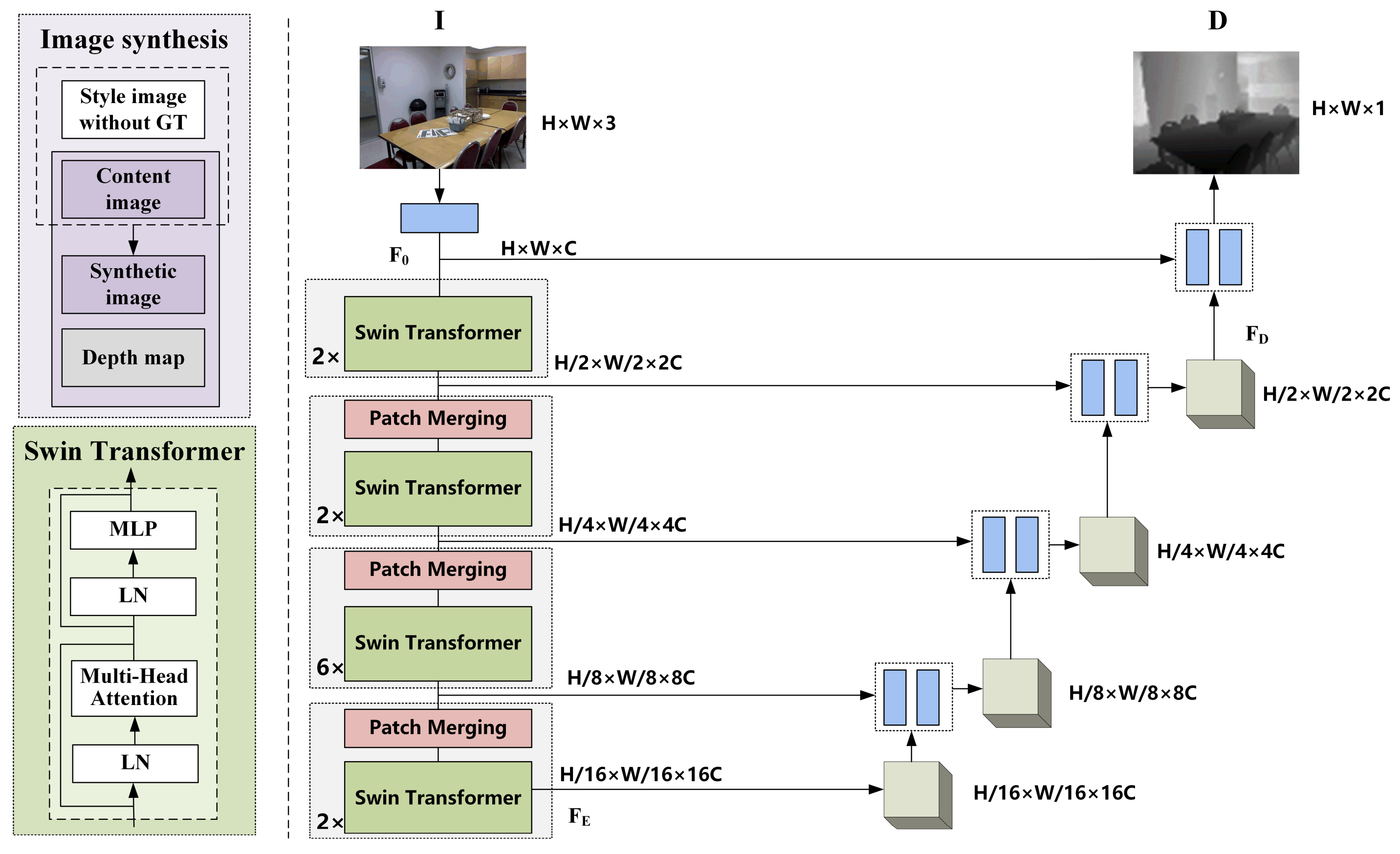
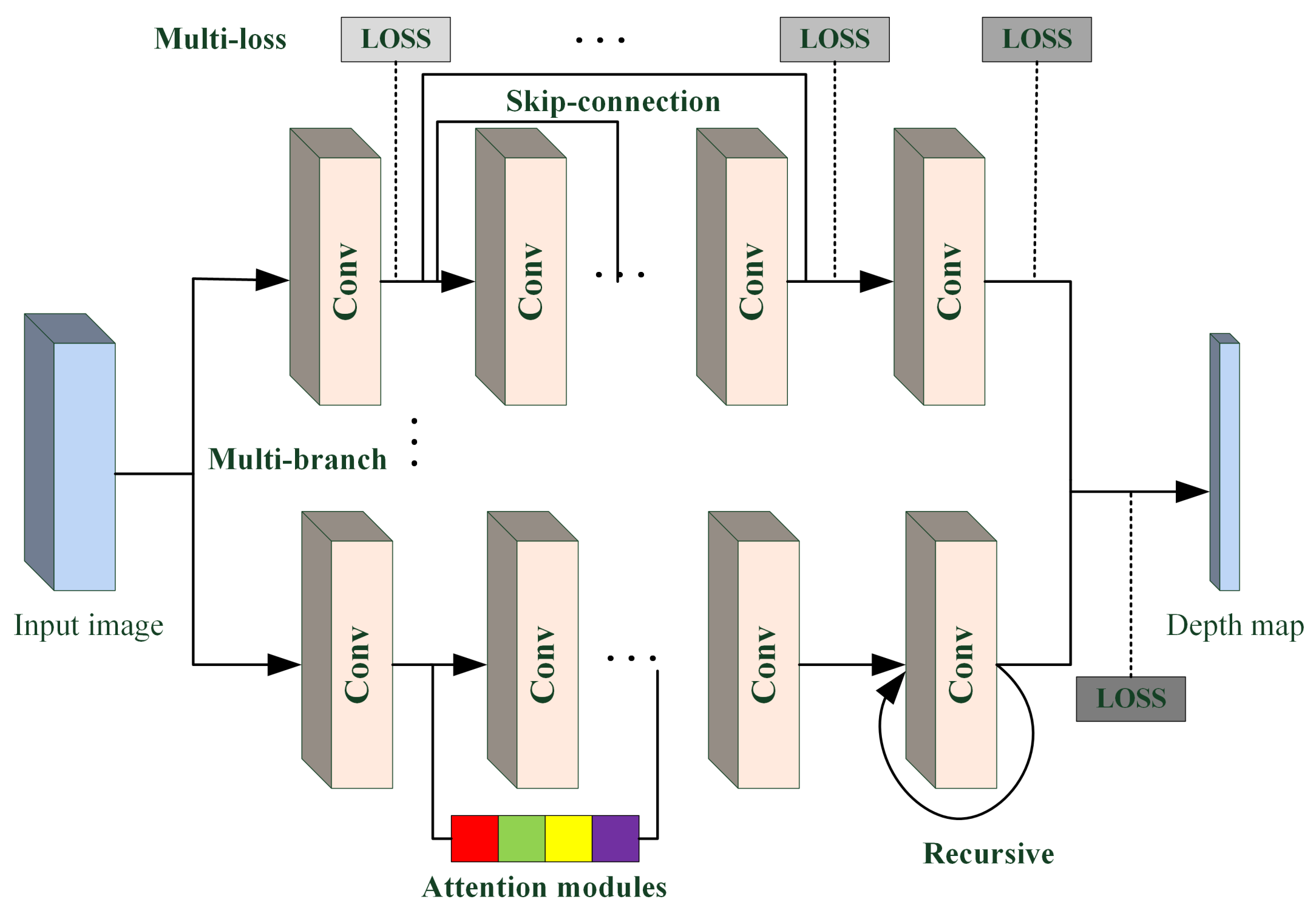
3.1. Image-Depth Estimation

3.1.1. Overall Pipeline

Image-depth estimation is to estimate the depth information of the object in the image at the time of actual shooting based on the RGB image. The model uses the U-Net [28] model structure which has excellent performance in the field of image segmentation. The encoder is used to continuously reduce the image size to obtain a larger perceptual field, and then the decoder is used to fuse the different scale features of the encoder to continuously recover the image size and learn the depth of objects in the image. The model architecture is shown in Figure 3.

Figure 3. Architecture of image-depth estimation. The encoder is composed of Swin Transformer [29] and the decoder consists of upsampling and convolutional layers.

To be specific, the input image $I\in {ℝ}^{H\times W\times 3}$ is given after the convolutional layer to obtain shallow features $F_0\in {ℝ}^{H\times W\times C}$. Then, the feature map is halved in width and height and doubled in feature channels for each Swin Transformer module, and the encoder output $F_E\in {ℝ}^{\frac{H}{16}\times \frac{W}{16}\times 4C}$. In the decoder part, the feature map is upsampled and fused with features from different Swin Transformer layers. The small-sized feature $F_E$ is gradually restored to a large-size $F_D\in {ℝ}^{\frac{H}{2}\times \frac{W}{2}\times 2C}$. Finally, a convolution layer is applied to refined features to generate the depth map $D\in {ℝ}^{H\times W\times 1}$.

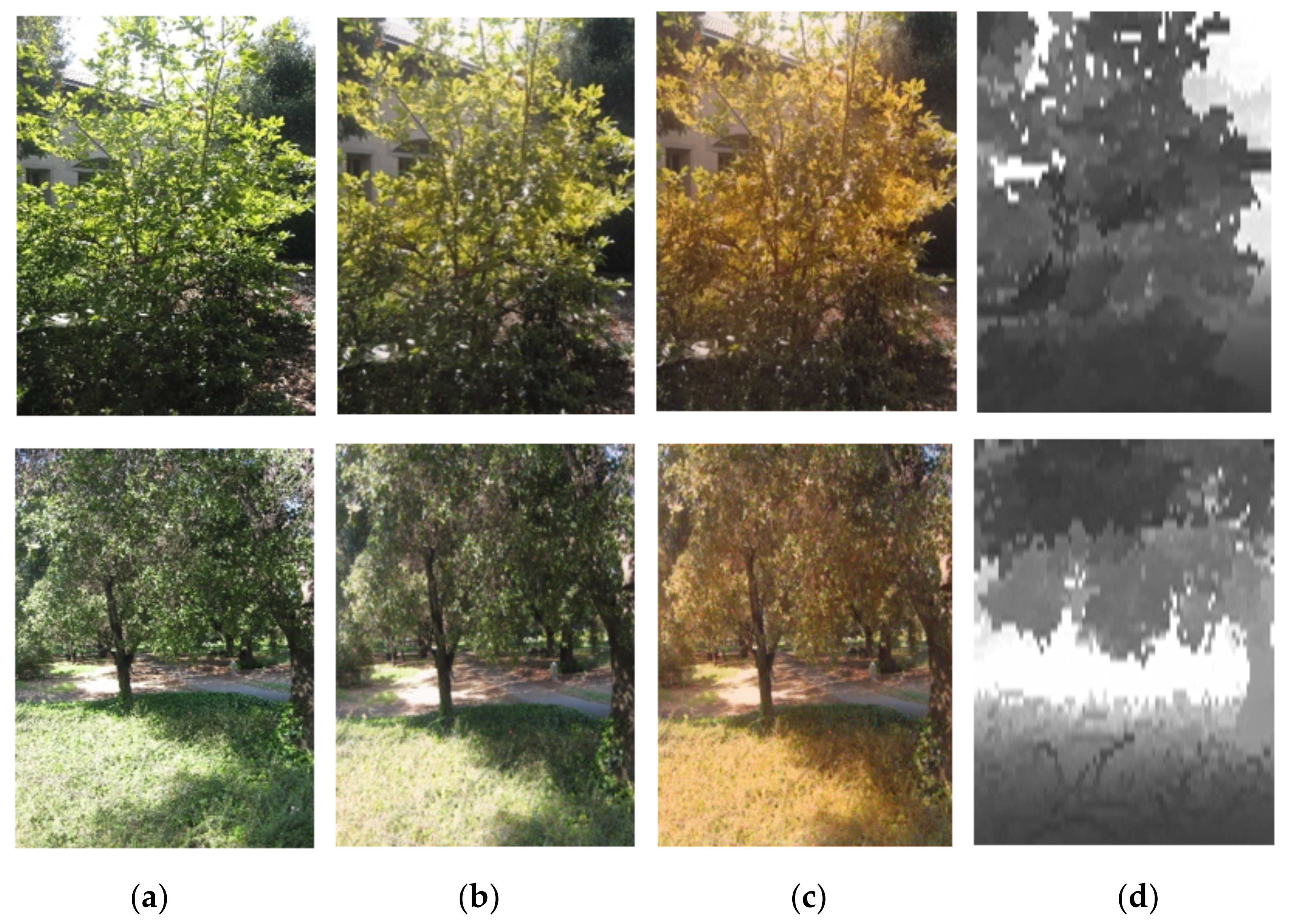
3.1.2. Image Synthesis

The acquisition of image-depth pairs is difficult, but the model does not perform well with limited training data. Therefore, we use the image-style transfer [30] to obtain synthetic images by using the image without depth map as the style image and the image with depth map as the content image. The purpose of image synthesis is twofold; one is to increase the amount of data, and the other is that we want the model to focus not only on the color edges of objects in the image for depth estimation, but we want the model to obtain the same depth information when estimating images with the same content but different styles. Figure 4 shows the synthesized images: the first column is the original image, the second and third columns are the synthesized images, and the fourth column is the depth map.

Figure 4. Synthetic-image display. (a) Original image; (b) synthesized image; (c) synthesized image; (d) depth map.

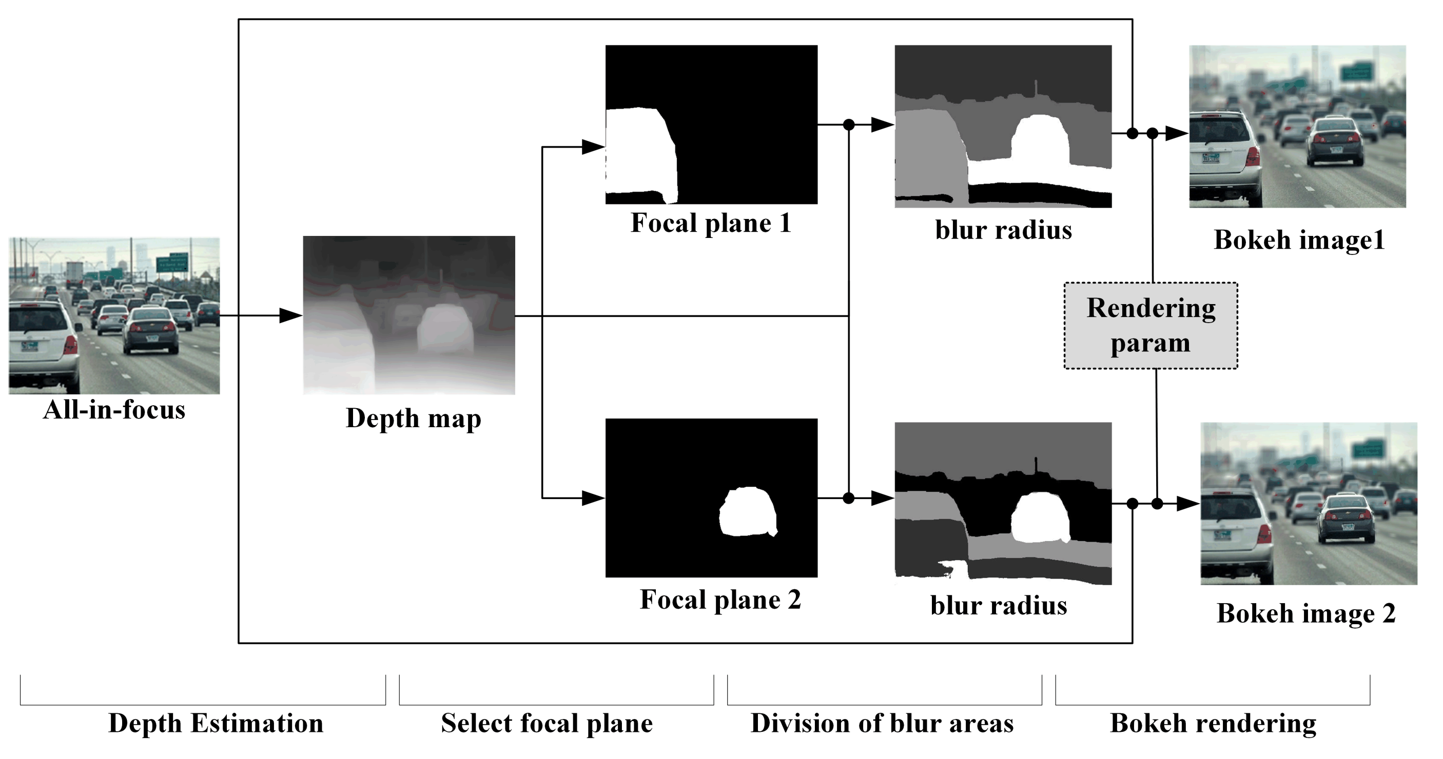
3.2. Bokeh-Effect Rendering

The bokeh effect is to bring the focus on the foreground object. To obtain a background bokeh effect when shooting, we need to take a photo with a large-aperture lens by focusing the camera on a selected area or object. When the camera parameters are not met or a cluttered background image has been obtained, image processing can be used to obtain it. The bokeh image obtained by means of image processing must be close to the image obtained directly using shooting techniques. Therefore, several characteristics of image bokeh must be satisfied when image processing: the foreground object (focal plane) should be clear; the object outside the focal plane should be blurred; and the further away from the focal plane the object is, the more blurred it is.

3.2.1. Uniform Bokeh Effects

After image-depth estimation, we obtain the depth information of the objects in the image. The distribution of pixels in the foreground and background is obtained by counting the distribution of depth and setting the mask according to the foreground target as:

$$Mask(x,y)=\left\{\begin{array}{c}255,foreground\\ 0,background\end{array}\right.$$

(1)

By directly blurring the background image with Gaussian, different degrees of blurring effect can be obtained by different blurring radii. The uniform bokeh effect with a strict division between foreground and background is obtained by Equation (2).

$$out=\frac{Mask}{255}*image+(1-\frac{Mask}{255})*Gblur(image)$$

(2)

where $image$ is the original image; $Gblur(image)$ means to apply Gaussian blur to $image$, calculated as:

$$Gblur(image)=image*G(x,y,\sigma )$$

(3)

where

$$G(x,y,\sigma )=\frac{1}{2\pi {\sigma }^2}\exp \left[-\frac{(x^2+y^2)}{2{\sigma }^2}\right]$$

(4)

The boundary between the foreground and background of the bokeh image obtained using Equation (2) is very obvious, and in order to make the boundary excessively smooth, the foreground and background boundaries need to be blurred, calculated as:

$$out=\frac{Gblur(Mask)}{255}*image+[1-\frac{Gblur(Mask)}{255}]*Gblur(image)$$

(5)

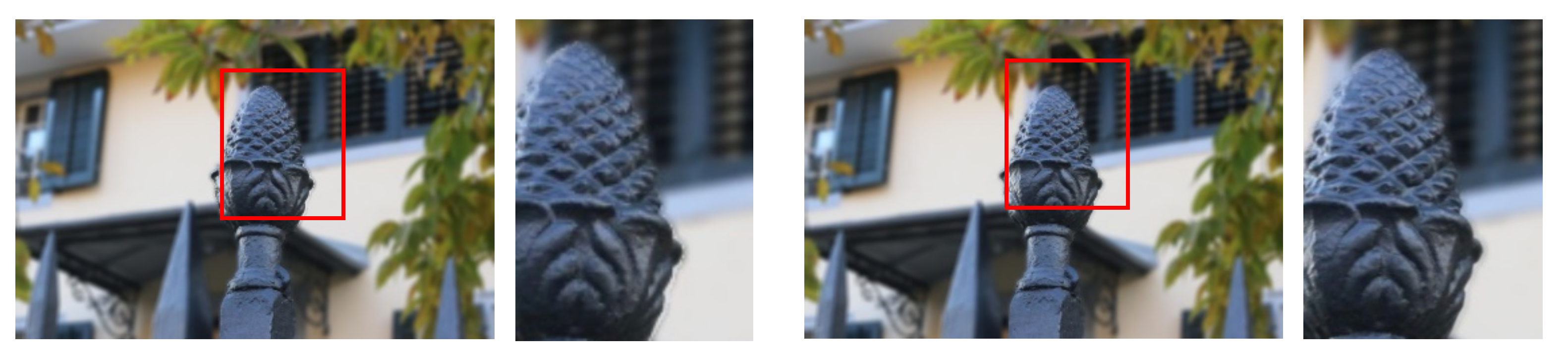
3.2.2. Natural Bokeh Effect

The bokeh image obtained using Equation (5) is a uniform bokeh effect, which does not take into account the fact that objects in the background become more blurred the farther they are from the focal plane. In order to acquire this effect, it is necessary to obtain the position of the focal plane. In the field of photography, the sharpest point of the scene image that the camera shoots is the focus; the main focus of the lens and a number of subfocus points constitute the plane perpendicular to the main axis, called the focal plane. In this paper, we define the focal plane as the plane in which the object that we want to be clear among all objects in the image is located. After the image-depth estimation, each pixel in the image will have a predicted depth value; in this paper, the depth value of the center of mass of the focal plane represents the depth of the focal plane.

Let the depth of the center-of-mass position of the focal plane be:

$$D_0=D(x_0,y_0)$$

(6)

Then the distance (the difference in the depth values) from the focal plane at any position $(x,y)$ in the image is:

$$D_{diff}=D(x,y)-D_0$$

(7)

The background blur is performed using a variable-radius Gaussian blur centered at the center of mass. Depending on the distance from the focal plane, the blur radius is defined as:

$$R=k{D}_{diff}$$

(8)

To ensure that objects are not oversegmented during background blurring, we use the same Gaussian blurring radius for points in a certain depth range, and k-means is used for clustering the depth range. For the same image, the clustering results are differently by choosing different focal planes, as shown in Figure 5.

Figure 5. Different clustering results for the same image. (a) The first column shows the all-in-focus image and depth map. (b) The second column shows the different focal planes. (c) The third column shows the different clustering results.

The average depth is used as the basis for calculating the Gaussian blur radius for each depth range, and the Gaussian blur radii used for different depth ranges are:

$$R_i=k*Normalization(D(x,y)-\frac{{\displaystyle \sum _{i=1}^N{D}_i}}{N})$$

(9)

where $N$ is the number of pixels, $Normlization(•)$ is the normalization process, and $k$ is the scale factor. The normalization process is calculated as:

$$Normalization(x)=\frac{x-X_{\min }}{X_{\max }-X_{\min }}$$

(10)

where $x$ is one value of the original dataset $X$. $X_{\max }$ and $X_{\min }$ are the maximum and minimum values of the original dataset.

Using the mask idea of uniform bokeh effect, the natural bokeh effect can be obtained by blurring the background of different depths with different Gaussian radii.

4. Experiments

In this section, we first evaluate the depth-estimation model, introduce the dataset and evaluation metrics, then compare our method with other methods and show the visualization results. Then, the process of bokeh rendering is analyzed in depth and the results are presented.

4.1. Evaluation of Depth-Estimation Model

4.1.1. Depth-Estimation Dataset and Evaluation Metrics

In this paper, we trained on KITTI [31], NYU depth V2 [32] and their synthetic datasets, and also tested on Make3D [33] dataset containing other real-world scenes in order to verify the generalization ability of the model. KITTI is the most common dataset with 93,000 pairs of images, all captured by a car carrying four high-resolution RGB cameras, two grayscale cameras, and a laser scanner with a maximum depth distance of 120 m. The NYU depth V2 dataset contains 1449 pairs of images, obtained from RGB cameras and Microsoft Kinect depth cameras, collecting RGB images and depth information for 464 different indoor scenes with a depth range of 0.5–10 m. The Make3D dataset was built by Stanford University and contains 534 pairs of images captured as daytime urban and natural landscape images.

The evaluation metrics of image-depth-estimation models are divided into two categories: error and accuracy. We used the same evaluation metrics as in [6]. The smaller the error the better, and the greater the accuracy (acc) the better. The errors include absolute relative error (abs.rel), mean-square relative error (sq.rel), root-mean-square error (RMSE), and logarithmic root-mean-square error (log RMSE). These metrics are calculated as follows:

$$acc:\%of{d}_{i}s.t.\max (\frac{d_i}{d_i^{GT}},\frac{d_i^{GT}}{d_i})=\delta <thr$$

(11)

$$abs.rel:\frac{1}{N}{\displaystyle \sum _{i\in N}\frac{d_i-d_i^{GT}}{d_i^{GT}}}$$

(12)

$$sq.rel:\frac{1}{N}{\displaystyle \sum _{i\in N}\frac{{‖d_i-d_i^{GT}‖}^2}{d_i^{GT}}}$$

(13)

$$RMSE:\sqrt{\frac{1}{N}{\displaystyle \sum _{i\in N}{‖d_i-d_i^{GT}‖}^2}}$$

(14)

$$\log RMSE:\sqrt{\frac{1}{N}{\displaystyle \sum _{i\in N}{‖\log (d_i)-\log (d_i^{GT})‖}^2}}$$

(15)

where $d_i$ is the predicted value, $d_i^{GT}$ is the true value, $N$ is the number of pixels, and $thr$ is the threshold, $thr={1.25}^m,m=1,2,3$.

4.1.2. Performance Evaluation

We compared the method proposed in this paper with ten existing models, including Eigen [6], Godard [34], PHN [11], T2Net [19], Xu [35], Pilzer [36], GASDA [18], SharinGAN [20], AgFU-Net [14], and EESP [37]. Table 1 shows the performance results of the model proposed in this paper with the other models in the KITTI dataset, and Table 2 shows the performance results of the model on the NYU depth V2 dataset. The comparison shows that the depth-estimation model proposed in this paper performs well in both the evaluation metrics of error analysis and accuracy analysis. CNN and GAN are model structures that have been performing well in the image domain, and other methods adopt them as model bases. The results of the comparison with other models fully illustrate the feasibility of Transformer and CNN fusion used in image-depth-estimation tasks.

Table 1. Comparison between our method and other methods on the KITTI dataset.

Models	Error				Accuracy
	abs.rel	sq.rel	RMSE	logRMSE	<1.25	<1.252	<1.253
Eigen	0.203	1.548	6.307	0.282	0.702	0.890	0.959
Godard	0.148	1.344	5.927	0.247	0.803	0.922	0.964
PHN	0.136	-	4.082	0.164	0.864	0.966	0.989
T2Net	0.168	1.119	4.674	0.243	0.772	0.912	0.996
Xu	0.132	0.911	-	0.162	0.804	0.945	0.981
Pilzer	0.142	1.123	5.785	0.239	0.795	0.924	0.968
GASDA	0.149	1.003	4.995	0.227	0.824	0.941	0.973
SharinGAN	0.109	0.673	3.770	0.190	0.864	0.954	0.981
AgFU-Net	0.1190	0.9219	5.033	0.211	0.851	0.947	0.977
EESP	0.1196	0.889	4.329	0.192	0.865	0.943	0.989
Ours	0.119	0.899	4.349	0.189	0.966	0.944	0.988

Table 2. Comparison between our method and other methods on the NYU depth V2 dataset.

Models	Error				Accuracy
	abs.rel	sq.rel	RMSE	logRMSE	<1.25	<1.252	<1.253
Eigen	0.215	0.212	0.907	0.285	0.611	0.887	0.971
PHN	0.169	-	0.573	-	0.785	0.943	0.981
T2Net	0.257	0.281	0.915	0.305	0.540	0.832	0.946
Xu	0.163	-	0.655	-	0.706	0.925	0.981
Ours	0.165	0.188	0.605	0.179	0.788	0.934	0.980

In order to verify the generalization ability of the models, we trained on the KITTI dataset and tested on the Make3D dataset. Table 3 shows the test results of some models on the Make3D dataset, where the Godard, T2Net, GASDA, and SharinGAN models use training sets that are not the Make3D dataset. Although the distributions of the KITTI dataset and the Make3D dataset are very different, the results show that the model still performs well on the Make3D dataset, which fully illustrates the feasibility of the model design and the strong generalization ability of the model. The experimental results show that the models with the same distribution of training and test datasets have much better results than those with different distributions, which illustrates the importance of uniform distribution of training and test data and the necessity of designing more general models.

Table 3. Comparison between our method and other methods on the Make3D dataset. T means that the training set is Make3D.

Models	Training Set	Error
		abs.rel	sq.rel	RMSE
PHN	T	0.179	-	4.32
Xu	T	0.174	-	4.27
Godard	F	0.398	4.723	7.801
T2Net	F	0.508	6.589	8.935
GASDA	F	0.403	6.709	10.424
SharinGAN	F	0.377	4.900	8.388
Ours	F	0.389	4.922	8.389

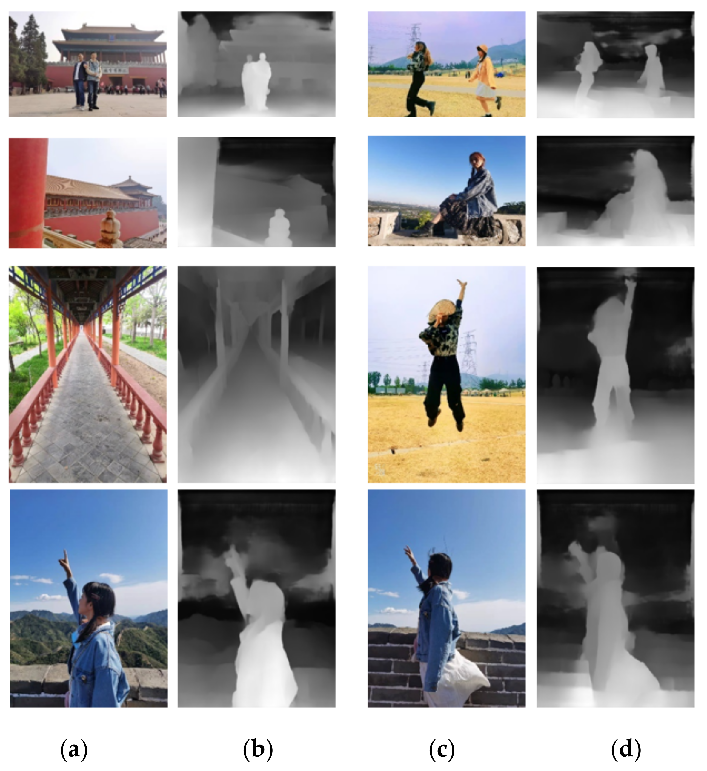
4.2. Image-Depth-Estimation Visualization

To visually demonstrate the performance of the image-depth-estimation model, we selected photos taken daily for image-depth estimation and visualized the depth map, as shown in Figure 6. The image on the right is the visualization result of the depth estimation of the RGB image on the left.

Figure 6. Image-depth-estimation visualization. (a) original image; (b) depth map; (c) original image; (d) depth map.

The results in Figure 6 show that the depth model can clearly distinguish the foreground and background, providing the possibility of rendering the image bokeh effect.

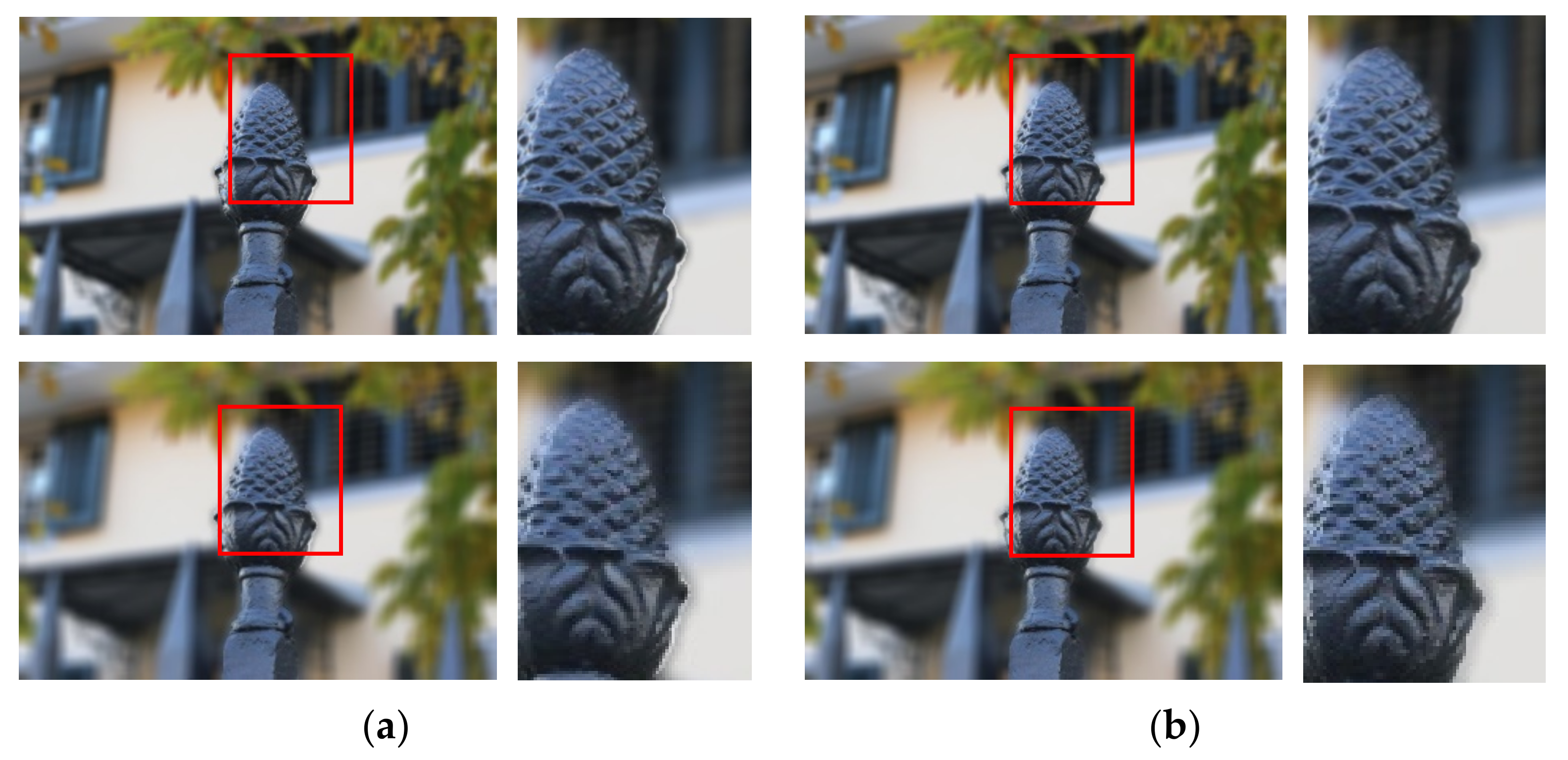
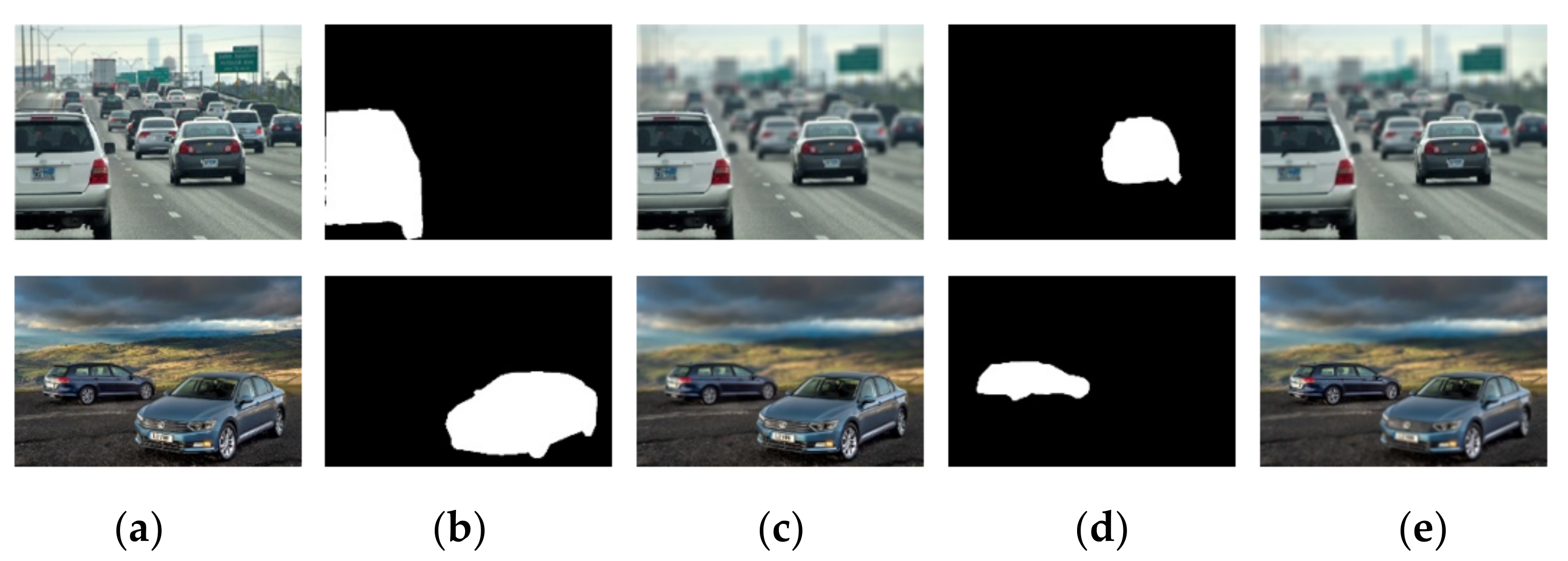
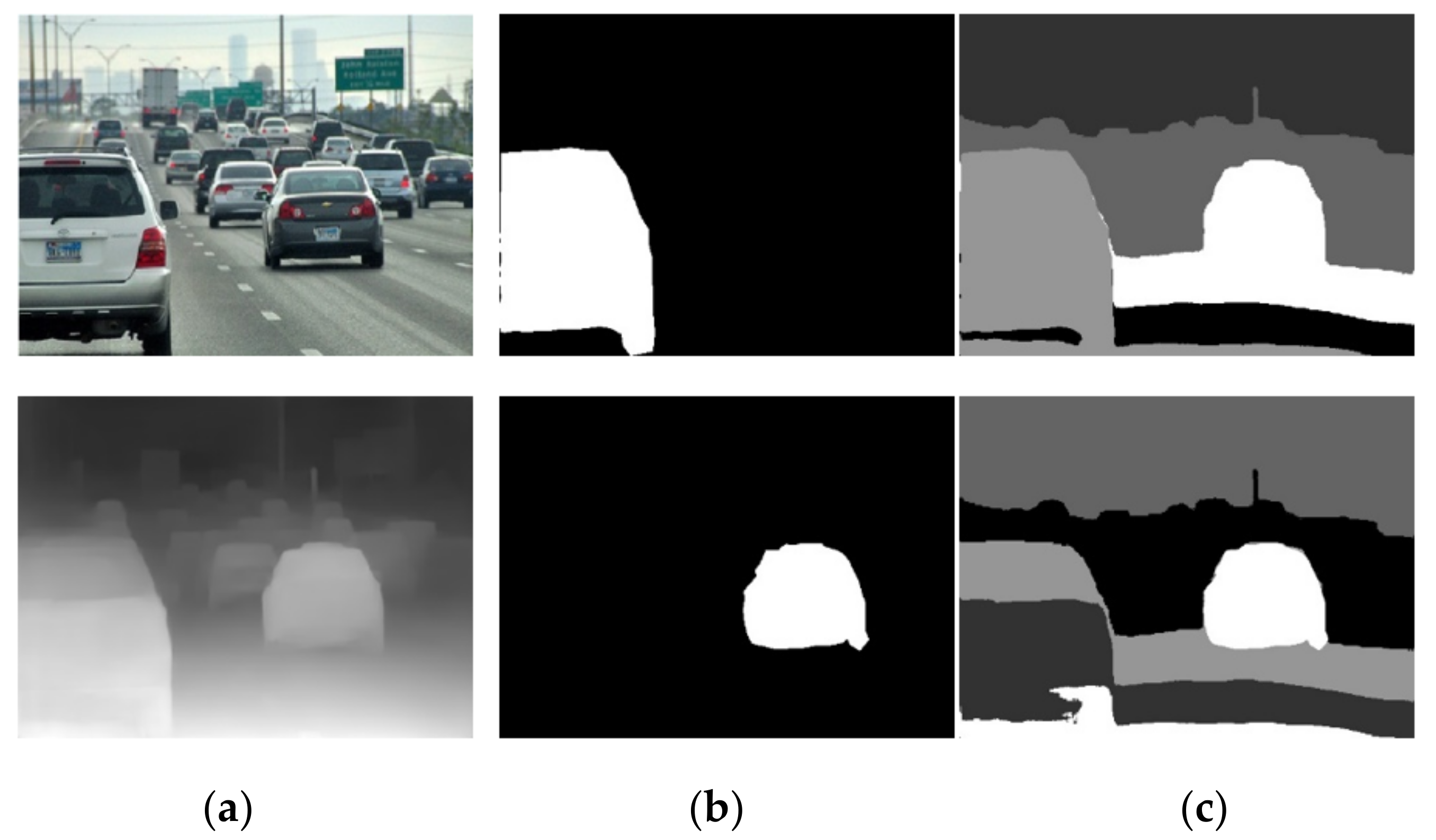
4.3. Visualization of Bokeh Effect

The uniform bokeh effect can clearly highlight the foreground object. The bokeh effect obtained by Equation (2) has a clear boundary between the foreground and the background, and the visualization effect is shown in Figure 7a, while the effect of Equation (3) to smooth the boundary is shown in Figure 7b. Figure 7 shows the uniform bokeh effect with different blurring degrees.

Figure 7. Uniform bokeh effect with Gaussian blur radius of 10, 15 and 20. (a) Uniform bokeh effect; (b) Uniform bokeh effect with smooth border.

The uniform bokeh effect only highlights the foreground object clearly, but it differs greatly from the real shot. A bokeh effect that conforms to the characteristic that objects in the background become more blurred the farther they are from the focal plane not only highlights the foreground objects clearly, but also gradually increases the blurring effect from near to far, making the aesthetic quality of the image higher. Figure 8 shows the comparison between the uniform bokeh effect and the natural bokeh effect, and the intermediate process results. In order to make the blurring degree similar, the Gaussian blurring radius of the uniform bokeh effect is the same as the scale factor of the natural bokeh effect, which is taken as $k=15$.

Figure 8. Comparison between the uniform bokeh effect and the natural bokeh effect, and the intermediate process results. (a) All-in-focus image; (b) depth map; (c) clustering result; (d) uniform bokeh; (e) natural bokeh.

The focal planes selected for the bokeh effect shown in Figure 8 are all objects in the middle of the image. When there are multiple main objects in the image, we can obtain different bokeh effect images by selecting different focal planes, as shown in Figure 9.

Figure 9. Bokeh images of different focal planes. (a) All-in-focus image; (b) focal planes 1; (c) bokeh image; (d) focal planes 2; (e) bokeh image.

5. Conclusions

In this paper, we proposed a method for single-image depth estimation, compared it with other methods, and tested it on photos taken by phone. We also proposed a method for rendering a natural bokeh effect based on k-means clustering, which can obtain images that are more consistent with the characteristics of the bokeh effect and satisfy the feature that objects are blurred the farther away they are from the focal plane. Our method can generate different bokeh images by choosing different focal planes. Since image-depth estimation and bokeh-effect rendering are independent of each other, the bokeh image will be more in line with the natural bokeh effect as the accuracy of the image-depth-estimation model becomes better and better.

References

1. León Araujo, H.; Gulfo Agudelo, J.; Crawford Vidal, R.; Ardila Uribe, J.; Remolina, J.F.; Serpa-Imbett, C.; López, A.M.; Patiño Guevara, D. Autonomous Mobile Robot Implemented in LEGO EV3 Integrated with Raspberry Pi to Use Android-Based Vision Control Algorithms for Human-Machine Interaction. Machines 2022, 10, 193. [Google Scholar] [CrossRef]
2. Vrochidou, E.; Oustadakis, D.; Kefalas, A.; Papakostas, G.A. Computer Vision in Self-Steering Tractors. Machines 2022, 10, 129. [Google Scholar] [CrossRef]
3. Lei, L.; Sun, S.; Zhang, Y.; Liu, H.; Xu, W. PSIC-Net: Pixel-Wise Segmentation and Image-Wise Classification Network for Surface Defects. Machines 2021, 9, 221. [Google Scholar] [CrossRef]
4. Wang, F.; Chen, J.; Zhong, H.; Ai, Y.; Zhang, W. No-Reference Image Quality Assessment Based on Image Multi-Scale Contour Prediction. Appl. Sci. 2022, 12, 2833. [Google Scholar] [CrossRef]
5. Shen, X.; Hertzmann, A.; Jia, J.; Paris, S.; Price, B.; Shechtman, E.; Sachs, I. Automatic Portrait Segmentation for Image Stylization. In Proceedings of the 37th Annual Conference of the European Association for Computer Graphics, Lisbon, Portugal, 9–13 May 2016; Eurographics Association: Goslar, Germany, 2016; pp. 93–102. [Google Scholar]
6. Eigen, D.; Puhrsch, C.; Fergus, R. Depth Map Prediction from a Single Image Using a Multi-Scale Deep Network. arXiv 2014, arXiv:1406.2283. [Google Scholar]
7. Eigen, D.; Fergus, R. Predicting Depth, Surface Normals and Semantic Labels with a Common Multi-Scale Convolutional Architecture. In Proceedings of the 2015 IEEE International Conference on Computer Vision (ICCV), Santiago, Chile, 7–13 December 2015; pp. 2650–2658. [Google Scholar]
8. Li, J.; Klein, R.; Yao, A. A Two-Streamed Network for Estimating Fine-Scaled Depth Maps from Single RGB Images; IEEE Computer Society: Washington, DC, USA, 2017; pp. 3392–3400. [Google Scholar]
9. Simonyan, K.; Zisserman, A. Very Deep Convolutional Networks for Large-Scale Image Recognition. arXiv 2004, arXiv:1409.1556. [Google Scholar]
10. Kim, Y.; Jung, H.; Min, D.; Sohn, K. Deep Monocular Depth Estimation via Integration of Global and Local Predictions. IEEE Trans. Image Processing 2018, 27, 4131–4144. [Google Scholar] [CrossRef] [PubMed]
11. Zhang, Z.; Xu, C.; Yang, J.; Gao, J.; Cui, Z. Progressive Hard-Mining Network for Monocular Depth Estimation. IEEE Trans. Image Processing 2018, 27, 3691–3702. [Google Scholar] [CrossRef] [PubMed]
12. Chen, Y.; Zhao, H.; Hu, Z.; Peng, J. Attention-Based Context Aggregation Network for Monocular Depth Estimation. Int. J. Mach. Learn. Cyber. 2021, 12, 1583–1596. [Google Scholar] [CrossRef]
13. Islam, N.U.; Park, J. Depth Estimation from a Single RGB Image Using Fine-Tuned Generative Adversarial Network. IEEE Access 2021, 9, 32781–32794. [Google Scholar] [CrossRef]
14. Lei, Z.; Wang, Y.; Li, Z.; Yang, J. Attention Based Multilayer Feature Fusion Convolutional Neural Network for Unsupervised Monocular Depth Estimation. Neurocomputing 2021, 423, 343–352. [Google Scholar] [CrossRef]
15. Garg, R.; Bg, V.K.; Carneiro, G.; Reid, I. Unsupervised CNN for Single View Depth Estimation: Geometry to the Rescue. In Proceedings of the Computer Vision-ECCV 2016; Leibe, B., Matas, J., Sebe, N., Welling, M., Eds.; Springer International Publishing: Cham, Switzerland, 2016; pp. 740–756. [Google Scholar]
16. Ye, X.; Ji, X.; Sun, B.; Chen, S.; Wang, Z.; Li, H. DRM-SLAM: Towards Dense Reconstruction of Monocular SLAM with Scene Depth Fusion. Neurocomputing 2020, 396, 76–91. [Google Scholar] [CrossRef]
17. Zhu, A.Z.; Yuan, L.; Chaney, K.; Daniilidis, K. Unsupervised Event-Based Learning of Optical Flow, Depth, and Egomotion. In Proceedings of the 2019 IEEE/CVF Conference on Computer Vision and Pattern Recognition (CVPR), Long Beach, CA, USA, 15–20 June 2019; pp. 989–997. [Google Scholar]
18. Zhao, S.; Fu, H.; Gong, M.; Tao, D. Geometry-Aware Symmetric Domain Adaptation for Monocular Depth Estimation. In Proceedings of the 2019 IEEE/CVF Conference on Computer Vision and Pattern Recognition (CVPR), Long Beach, CA, USA, 15–20 June 2019; pp. 9780–9790. [Google Scholar]
19. Zheng, C.; Cham, T.-J.; Cai, J. T2Net: Synthetic-to-Realistic Translation for Solving Single-Image Depth Estimation Tasks. In Proceedings of the Computer Vision-ECCV 2018; Ferrari, V., Hebert, M., Sminchisescu, C., Weiss, Y., Eds.; Springer International Publishing: Cham, Switzerland, 2018; pp. 798–814. [Google Scholar]
20. Pnvr, K.; Zhou, H.; Jacobs, D. SharinGAN: Combining Synthetic and Real Data for Unsupervised Geometry Estimation. In Proceedings of the 2020 IEEE/CVF Conference on Computer Vision and Pattern Recognition (CVPR), Seattle, WA, USA, 13–19 June 2020; pp. 13971–13980. [Google Scholar]
21. Qi, X.; Liao, R.; Liu, Z.; Urtasun, R.; Jia, J. GeoNet: Geometric Neural Network for Joint Depth and Surface Normal Estimation. In Proceedings of the 2018 IEEE/CVF Conference on Computer Vision and Pattern Recognition, Salt Lake City, UT, USA, 18–23 June 2018; pp. 283–291. [Google Scholar]
22. Yan, H.; Zhang, S.; Zhang, Y.; Zhang, L. Monocular Depth Estimation with Guidance of Surface Normal Map. Neurocomputing 2018, 280, 86–100. [Google Scholar] [CrossRef]
23. Huang, K.; Qu, X.; Chen, S.; Chen, Z.; Zhao, F. Superb Monocular Depth Estimation Based on Transfer Learning and Surface Normal Guidance. Sensors 2020, 20, 4856. [Google Scholar] [CrossRef] [PubMed]
24. Purohit, K.; Suin, M.; Kandula, P.; Ambasamudram, R. Depth-Guided Dense Dynamic Filtering Network for Bokeh Effect Rendering. In Proceedings of the 2019 IEEE/CVF International Conference on Computer Vision Workshop (ICCVW), Seoul, Korea, 27–28 October 2019; pp. 3417–3426. [Google Scholar]
25. Dutta, S.; Das, S.D.; Shah, N.A.; Tiwari, A.K. Stacked Deep Multi-Scale Hierarchical Network for Fast Bokeh Effect Rendering from a Single Image. In Proceedings of the 2021 IEEE/CVF Conference on Computer Vision and Pattern Recognition Workshops (CVPRW), Nashville, TN, USA, 19–25 June 2021; pp. 2398–2407. [Google Scholar]
26. Ignatov, A.; Patel, J.; Timofte, R. Rendering Natural Camera Bokeh Effect with Deep Learning. In Proceedings of the 2020 IEEE/CVF Conference on Computer Vision and Pattern Recognition Workshops (CVPRW), Seattle, WA, USA, 14–19 June 2020; pp. 1676–1686. [Google Scholar]
27. Choi, M.-S.; Kim, J.-H.; Choi, J.-H.; Lee, J.-S. Efficient Bokeh Effect Rendering Using Generative Adversarial Network. In Proceedings of the 2020 IEEE International Conference on Consumer Electronics-Asia (ICCE-Asia), Seoul, Korea, 1–3 November 2020; pp. 1–5. [Google Scholar]
28. Ronneberger, O.; Fischer, P.; Brox, T. U-Net: Convolutional Networks for Biomedical Image Segmentation; Springer: Berlin/Heidelberg, Germany, 2015. [Google Scholar]
29. Liu, Z.; Lin, Y.; Cao, Y.; Hu, H.; Wei, Y.; Zhang, Z.; Lin, S.; Guo, B. Swin Transformer: Hierarchical Vision Transformer Using Shifted Windows. arXiv 2021, arXiv:2103.14030. [Google Scholar]
30. Huang, X.; Belongie, S. Arbitrary Style Transfer in Real-Time with Adaptive Instance Normalization. In Proceedings of the 2017 IEEE International Conference on Computer Vision (ICCV), Venice, Italy, 22–29 October 2017; pp. 1510–1519. [Google Scholar]
31. Geiger, A.; Lenz, P.; Urtasun, R. Are We Ready for Autonomous Driving? The KITTI Vision Benchmark Suite. In Proceedings of the 2012 IEEE Conference on Computer Vision and Pattern Recognition, Washington, DC, USA, 16–21 June 2012; pp. 3354–3361. [Google Scholar]
32. Silberman, N.; Hoiem, D.; Kohli, P.; Fergus, R. Indoor Segmentation and Support Inference from RGBD Images. In Proceedings of the European Conference on Computer Vision; Springer: Berlin/Heidelberg, Germany, 2012; Volume 7576, pp. 746–760. [Google Scholar]
33. Saxena, A.; Chung, S.H.; Ng, A.Y. Learning Depth from Single Monocular Images. In Proceedings of the 18th International Conference on Neural Information Processing Systems, Cambridge, MA, USA, 5–8 December 2005; MIT Press: Cambridge, MA, USA, 2005; pp. 1161–1168. [Google Scholar]
34. Godard, C.; Aodha, O.M.; Brostow, G.J. Unsupervised Monocular Depth Estimation with Left-Right Consistency. In Proceedings of the 2017 IEEE Conference on Computer Vision and Pattern Recognition (CVPR), Honolulu, HI, USA, 21–26 July 2017; pp. 6602–6611. [Google Scholar]
35. Xu, D.; Ricci, E.; Ouyang, W.; Wang, X.; Sebe, N. Monocular Depth Estimation Using Multi-Scale Continuous CRFs as Sequential Deep Networks. IEEE Trans. Pattern Anal. Mach. Intell. 2019, 41, 1426–1440. [Google Scholar] [CrossRef] [PubMed] [Green Version]
36. Pilzer, A.; Lathuilière, S.; Sebe, N.; Ricci, E. Refine and Distill: Exploiting Cycle-Inconsistency and Knowledge Distillation for Unsupervised Monocular Depth Estimation. In Proceedings of the 2019 IEEE/CVF Conference on Computer Vision and Pattern Recognition (CVPR), Long Beach, CA, USA, 15–20 June 2019; pp. 9760–9769. [Google Scholar]
37. Bhattacharyya, S.; Shen, J.; Welch, S.; Chen, C. Efficient Unsupervised Monocular Depth Estimation Using Attention Guided Generative Adversarial Network. J. Real-Time Image Proc. 2021, 18, 1357–1368. [Google Scholar] [CrossRef]
Publisher’s Note: MDPI stays neutral with regard to jurisdictional claims in published maps and institutional affiliations.
Article Metrics
Citations
Article Access Statistics
Multiple requests from the same IP address are counted as one view.