Article

A Lightweight Two-End Feature Fusion Network for Object 6D Pose Estimation

School of Computer and Communication Engineering, University of Science and Technology Beijing, Beijing 100083, China
*
Author to whom correspondence should be addressed.
Machines 2022, 10(4), 254; https://doi.org/10.3390/machines10040254
Submission received: 27 February 2022 / Revised: 29 March 2022 / Accepted: 29 March 2022 / Published: 1 April 2022
(This article belongs to the Section Robotics, Mechatronics and Intelligent Machines)

Abstract

:
Currently, many methods of object pose estimation use images or point clouds alone for pose estimation. This leads to their inability to accurately estimate the object pose in the case of occlusion and poor illumination. Second, these models have large parameters and cannot be deployed on mobile devices. Therefore, we propose a lightweight two-terminal feature fusion network, which can effectively use images and point clouds for accurate object pose estimation. First, Pointno problemNet network is used to extract point cloud features. Then the extracted point cloud features are combined with the images at pixel level and the features are extracted by CNN. Secondly, the extracted image features are combined with the point cloud point by point. Then feature extraction is performed on it using the improved PointNet++ network. Finally, a set of center point features are obtained and pose estimation is performed for each feature. The pose with the highest confidence is selected as the final result. Furthermore, we apply depthwise separable convolutions to reduce the amount of model parameters. Experiments show that the proposed method exhibits better performance on Linemod and Occlusion Linemod datasets. Furthermore, the model parameters are small, and it is robust in occlusion and low-light situations.

1. Introduction

Pose estimation of objects is a core task for many computer vision applications, such as robotic automated operations, augmented reality, and autonomous driving. It has become a popular research topic for many research institutions. The main objective of object pose estimation is to calculate the rotation matrix and translation vector of the target object in the camera coordinate system. Earlier methods only used RGB images for object pose estimation. This limits the performance of these methods in scenes with occlusions, poor illumination, low background contrast, and untextured objects. Recently, the advent of cheap RGBD cameras has prompted some researchers to use RGBD images to accurately estimate the pose of textureless objects. However, these methods not only have a large number of parameters and low real-time performance, they do not make full use of the depth information, which leads to the poor performance of these methods in low light and occlusion conditions. Therefore, we believe that making full use of color and depth information for pose estimation is the core problem of current research work.
Traditional pose estimation methods can be generally classified into two categories: correspondence-based methods [1,2,3,4,5] and template-based methods [6,7,8,9,10]. Correspondence-based methods first extract 2D keypoints from RGB images, then establish the correspondence between 2D and 3D keypoints, and finally estimate the object pose through the PnP [11] algorithm. However, 2D keypoints cannot be accurately extracted for objects lacking texture. Therefore, these methods perform poorly on objects that lack texture. Template-based methods compare the gradient information of the real image and the template image. The template image that most closely resembles the real image can be found. The 6D pose corresponding to the template image is taken as the 6D pose of the current target object. This type of method is mainly aimed at the pose estimation of objects lacking texture, which makes up for the shortcomings of the correspondence-based method. However in the case of occlusion, such methods can significantly degrade the performance of template matching.
With the rapid development of deep learning technology. Convolutional Neural Networks (CNN) are widely used in image processing tasks, such as object detection [12] and image classification [13]. Therefore, it has also motivated some researchers to use CNN to solve the object 6D pose estimation problem. CNN-based methods are mainly divided into two categories. One category uses CNN to detect 2D keypoints in RGB images [14,15,16,17,18,19,20,21], which solves the keypoint detection problem that traditional methods are not suitable for textureless objects. However, it does not accurately estimate the object pose in the case of occlusion. Another class of methods is to directly use RGB images to regress the 6D pose of objects, such as PoseNet [22], PoseCNN [23] and SSD-6D [24]. The object pose estimated by these methods is usually inaccurate, and time-consuming iterative algorithms (such as ICP [25]) are required later for pose optimization. The above two types of methods just use RGB images to estimate the object pose. They do not use depth information or combine color and depth information for positional estimation. Regarding the problem of occlusion, Fractal Markers [26] address the estimation of marker poses under occlusion by detecting key points, and Body PointNet [27] directly processes point cloud data to estimate 3D body shapes and poses under clothing. These methods can better solve the problem of pose estimation under occlusion. Recently, Densefusion [28] combined color and depth information for the first time to estimate object 6D poses, with better performance under occlusion and low illumination. It extracts RGB and point cloud features through CNN and PointNet [29], respectively. Then pixel-level fusion of image features and point cloud features is performed to regress the object pose. However, this method employs separate networks to extract RGB and point cloud information separately. It does not fully fuse the two kinds of information in the feature extraction process. Secondly, the above method has a large amount of parameters, which is not conducive to deployment on mobile devices.
In this work, we propose a lightweight two-terminal feature fusion pose estimation network. It can fully integrate RGB and point cloud information in the feature extraction process, and the amount of network parameters is small, which is easy to deploy on mobile devices. The core of the method is a two-end feature fusion network, where point cloud features and color features can be used as supplementary information on the other side during feature extraction. Specifically, during CNN encoding-decoding, it is difficult for CNNs to extract unique features of similar objects from RGB images, however, the same is true for point cloud networks. On the other hand, in the case of dark or strong light, the color information of the picture will be lost. Objects with reflective surfaces can cause loss of depth information. Therefore, our method first uses the PointNet network to extract the point cloud features of the target object, then uses the point cloud features as the geometric supplementary information of the RGB image to perform pixel-level stitching, and uses CNN to perform feature extraction on the stitched images. Second, the extracted image features are combined point by point as the color supplementary information of the point cloud, and the improved PointNet++ [30] network is used for feature extraction. Then a set of center point features are obtained and pose estimation is performed, and the pose with the highest confidence is selected as the final result. Finally, we use a pose iterative module to further improve the accuracy of pose estimation. Furthermore, we apply depthwise separable convolutions to reduce the amount of model parameters, facilitating the model deployment on mobile devices. The proposed method is evaluated on two benchmark datasets, Linemod [6] and Occlusion Linemod [31], and our method exhibits better performance on both datasets.
In summary, the contributions of our work are as follows:
(1)
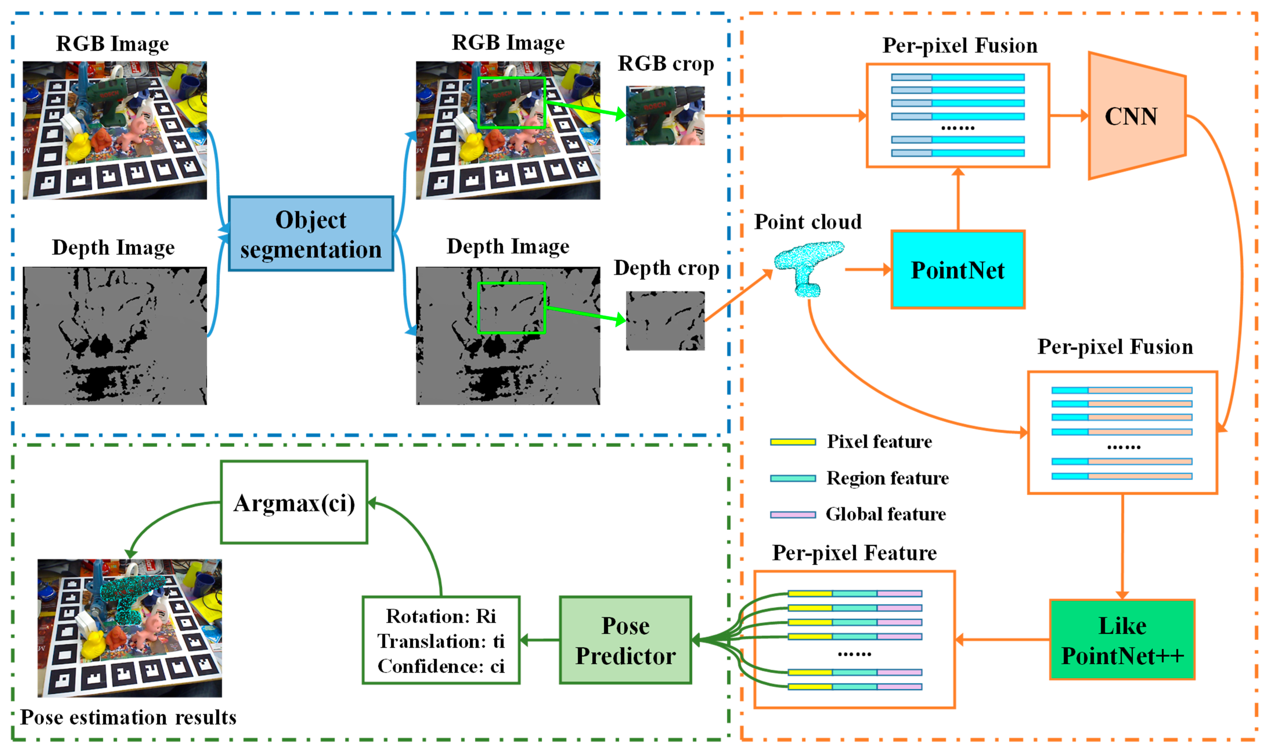
A two-end feature fusion pose estimation network is proposed, which can fully fuse RGB and point cloud features to estimate object pose, and can handle the pose estimation problem in the occlusion case.
(2)
The depthwise separable convolution is integrated into the 6D pose estimation network, thus reducing the model storage space and speeding up the model inference, and better results are obtained.
(3)
Better performance of 6D pose estimation is achieved on Linemod and Occlusion Linemod datasets.

2. Related Work

2.1. Template-Based Methods

The core of the template-based approach is template matching, which searches for the best match in the template dataset by means of a sliding window. Each template is labeled with the exact 6D pose of the object. When the best template is found, the 6D pose of the object is also determined. Therefore, the template-based 6D pose estimation problem is transformed into an image retrieval problem. The Linemod [6] method is a representative method based on templates. It matches the color gradient and surface normal vector of the template image with the color gradient and surface normal vector of the real image, and finally obtains the 6D pose of the target object. Rios-Cabrera et al. [7] propose a real-time scalable method. The method accelerates detection speed through a cascaded scheme, and can quickly and accurately match a large number of objects. Sundermeyer et al. [9] proposed an implicit template matching method. It encodes tens of thousands of template images to form a codebook, inputs real images for encoding, forms a code and compares the codebook to find the most similar template. However, these methods perform poorly in occlusion situations.

2.2. Correspondence-Based Methods

The correspondence-based method is mainly to solve the problem of estimating the pose of texture-rich objects. The core step of this method is to project the 3D model to N angles, obtain N RGB template images, and record the correspondence between 2D pixel points and 3D model points. Next, we obtain a single real RGB image, and use the feature point extraction algorithms SURF [1], ORB [4], SIFT [5] to obtain the 2D key point correspondence between the real image and the template image. The 2D-3D keypoint correspondence is established by the template, and finally the PnP algorithm is used to calculate the object pose. However, the traditional feature point extraction algorithm is not applicable to the objects lacking textures. To solve this problem, some researchers employ CNN to extract keypoints. YoLo6D [16] uses YOLO architecture to predict the 2D image position of object 3D bounding box projection vertices in real time, and the final pose is obtained by PnP algorithm. DPOD [17] is to estimate the dense multi-class 2D-3D correspondence map between the input image and the known 3D model. According to the given correspondence, the PnP and RANSAC algorithms are used for 6D pose estimation. Hu et al. [18] proposed a segmentation-driven 6D pose estimation framework, in which each visible part of the object contributes towards the local pose prediction in the form of 2D key point locations, which can solve multiple objects with poor texture that are occluded from each other. PVNet [19] proposed a pixel-by-pixel voting network based on the RANSAC algorithm to determine keypoint locations, and then use 2D-3D correspondences to estimate object poses. HybridPose [20] adds edge vectors and symmetric correspondences in the PVNet framework, which can enhance the robustness of symmetric object pose estimation. However, the above approach requires advance definition of key points in the 3D model and is not very real-time.

2.3. RGBD-Based Methods

Traditional methods extract manual features from RGBD images with corresponding grouping and hypothesis validation [8,32,33,34,35]. The method proposed by Hinterstoisser et al. [8] estimates object pose by extracting gradient features from RGB images and normal features from depth images. However, their performance is limited in situations with strong illumination changes and severe occlusion. Some researchers use CNN to directly process image data and estimate object pose [23,24,36,37,38]. Among them, PoseCNN [23] uses RGB images to estimate the initial pose, and optimizes the object pose through object point cloud and ICP algorithm. SSD6D [24] extends the SSD detection network to achieve 6D pose estimation of objects, and also uses an iterative algorithm to optimize the pose. The above two methods have poor real-time performance and cannot perform end-to-end training and estimate object poses. Li et al. [36] used a CNN network to extract RGB image and depth image features, and then stitched the depth image features as supplementary channels of RGB images to estimate object pose. However, it ignores the internal structure of the depth channel, and does not fully utilize the RGBD information. Recently, several researchers have performed a feature fusion of depth and RGB maps to estimate object pose [28,39,40,41,42,43]. Among them, Densefusion [28] is the most representative method. It first converts depth images into point cloud data, and then uses CNN and PointNet to extract features from RGB images and point clouds, respectively. Then, a dense pixel-level fusion method is designed, which integrates RGB image features and point cloud features to estimate the pose of the object, which can solve the problem of pose estimation under occlusion. This method uses two kinds of data quickly and efficiently to estimate object pose. PVN3D [39] uses the Densefusion architecture to fuse RGB and point cloud information, and then generates 3D keypoints through an all-pixel voting network. Finally, the least squares method is used to calculate the 6D pose, and the pose estimation problem under occlusion is solved by detecting the 3D key points of the object. Zhou et al. [40] used PointNet++ network to process the fused features of point clouds and images, and then estimated the object pose by multiple region-level features to solve the pose estimation problem under occlusion. However, color features and geometric features are extracted separately, and the two features are not well integrated in the extraction process, and these methods have a large number of parameters. Therefore, we propose a lightweight two-end feature fusion network to fully fuse the two kinds of data. It uses the feature extraction results of one side of the data as the complementary information to the other side of the data for feature extraction. This can well fuse the two kinds of data to estimate the object pose during the feature extraction.

3. Methodology

In this work, we propose a method for object 6D pose estimation, where the main task is to predict the pose of an object in a 3D space from an RGBD image. It represents the rotation matrix and translation vector of the object in the camera coordinate system. We believe that only the color and depth information can be fully integrated in the feature extraction process. This can solve the problem of pose estimation under conditions, such as occlusion and poor illumination. How to effectively fuse them and reduce the number of model parameters is a problem that needs to be faced in the current research. Therefore, we propose a lightweight two-end feature fusion network to fully fuse these two features. We also integrate deep separable convolution into the network to reduce the number of model parameters.
The algorithm framework proposed in this paper is shown in Figure 1, and it consists of three main parts. Among them, the first part is the semantic segmentation of RGB images. Obtain the bounding box of the target object and crop it, get only the color map and depth map of the target object, and convert the depth map into a point cloud. The second part is the feature extraction structure. Firstly, the PointNet network is used for the feature extraction of the object point clouds, and then the point cloud features are stitched at the pixel level as information that is geometrically complementary to the RGB images. The stitched images are then inputted into CNN for feature extraction. After that, the obtained color features are combined point by point as the color complementary information of the point cloud. Then the improved PointNet++ network is used for feature extraction of the combined point cloud. Finally, a set of centroid features fused by pixel features, area features, and global features are obtained. In the third part, the poses are estimated for each centroid feature and the poses with the highest confidence are the output. Finally, we refer to the pose iterative module in [28] to improve the accuracy of pose estimation.

3.1. Semantic Segmentation

The first task of our network framework is semantic segmentation. Its purpose is to crop the target object from the RGBD image, and finally generate a color image and a depth image containing only the target object. Today, semantic segmentation research is very mature, such as in [44]. The semantic segmentation framework is mainly composed of an encoder and a decoder, which encodes and decodes color images and generates a result map with N + 1 channels. The first channel represents the background of the image, and the other N channels represent the class of the known target object. Therefore, we directly use the semantic segmentation network in PoseCNN to crop the image.

3.2. Image Feature Extraction and Feature Fusion

A color image block of size h   ×   w   ×   3 containing only the target object is obtained through a semantic segmentation network. Then, the PointNet network is used to extract features from the point cloud of the target object and the extracted point cloud features are used as geometric supplementary information of color image pixels. According to the pixel position correspondence between the depth map and the color map, the color image and point cloud features are stitched at the pixel level along the channel dimension. Finally, a picture of size h   ×   w   ×   ( 3 + d p ) with geometric features per pixel is obtained, where d p is the number of channels of the geometric features. To be able to use the feature extraction results for point-level feature fusion with the point cloud, we employ an upsampling module that keeps the output feature map the same size as the input image. Therefore, we refer to the image feature extraction method in [28] to build an image feature extraction network structure, which is composed of ResNet [13], PSPNet [45] and an upsampling module. Its structure is shown in Figure 2. Among them, the ResNet network preprocesses the image, then uses the PSPNet network for multi-scale feature extraction, and finally uses the upsampling module to keep the input and output sizes the same.
The image of size h   ×   w   ×   ( 3 + d p ) , is preprocessed by the ResNet network, and the feature map of size h 1   ×   w 1   ×   d 1 can be obtained, and again the feature map of size h 2   ×   w 2   ×   d r g b p is obtained by feature extraction of the PSPNet network. Finally, the feature map is upsampled by the bilinear interpolation function, and the feature map of size h   ×   w   ×   d r g b p is finally obtained.

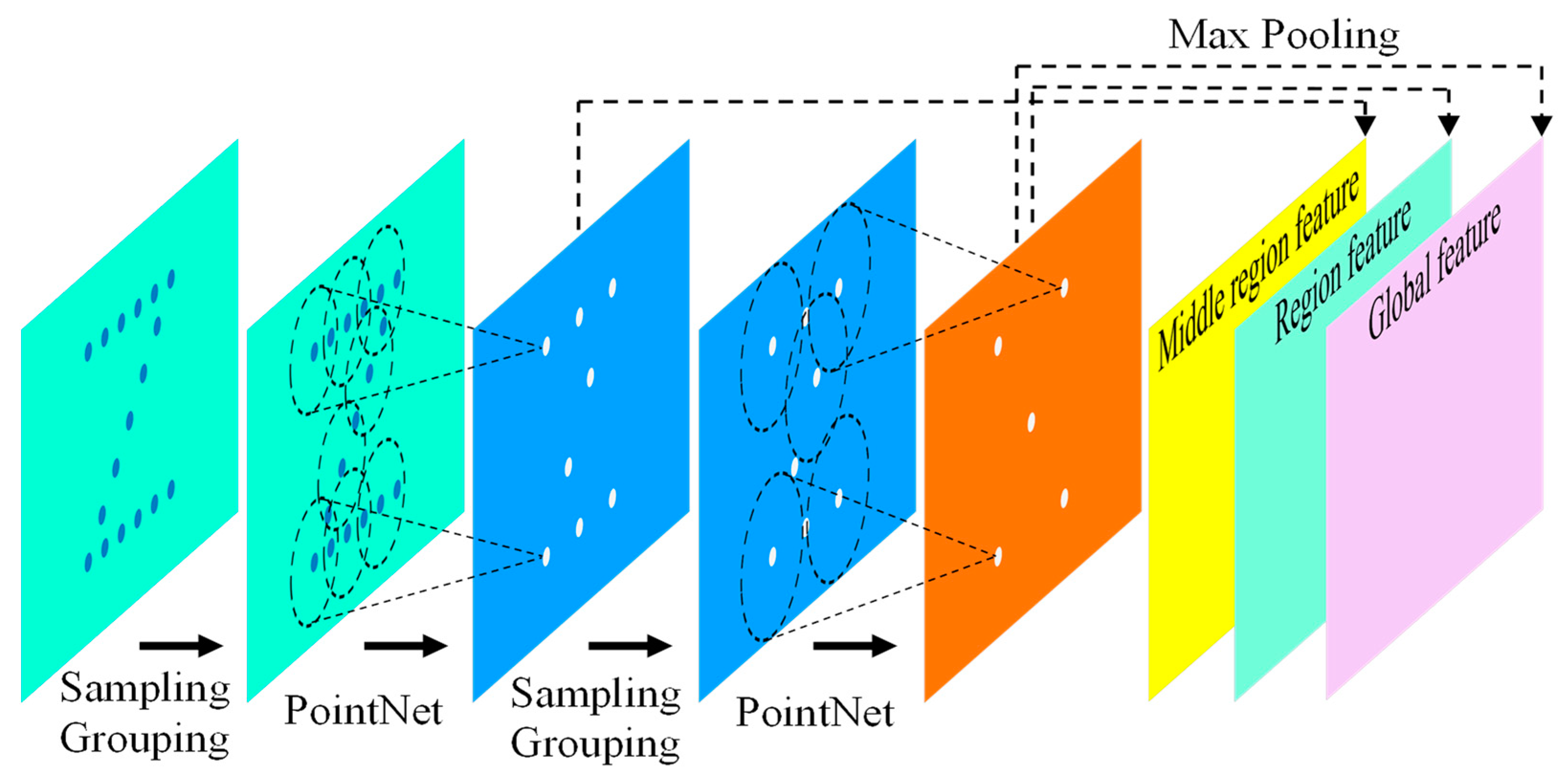
3.3. Point Cloud Feature Extraction and Feature Fusion

This method has two point cloud feature extraction networks, which can fully integrate color information and depth information. In the first part, geometric information is added to each RGB image pixel point before RGB image feature extraction. First, the depth map cropped by the semantic segmentation network is converted into a point cloud. The location ( u ,   v ) of each pixel point in the depth map is transformed into a 3D point ( x ,   y ,   z ) in the point cloud according to the camera parameters. The specific calculation is:
z = d t   /   s x = ( u     c x ) ×   z   /   f x y = ( v     c y ) ×   z   /   f y
where d t represents the depth data at pixel location ( u ,   v ) , s is the camera scale factor, ( c x ,   c y ) stands for the camera’s aperture center coordinate and ( f x ,   f y ) is the focal length of the camera on the x and y axis.
We use a simple PointNet network for the initial feature extraction of point clouds. The point cloud of size N   ×   3 is inputted into PointNet, where N represents the number of point clouds and three represents the 3D coordinates. The final network output is:
I p = h ( h ( x 1 , x 2 , , x n ) ( M A X i = 1 , , n { h ( x i ) } ) )
where I p   denotes point cloud features of size N   ×   d p ,   d p stands for feature vector size, h denotes shared multilayer perceptron (MLP) network, MAX is the maximum pooling function and denotes point-level stitching. The final generated point cloud features have per-point features and global features. The extracted point cloud features are used as the geometric supplementary information of the color image to perform pixel-level fusion to obtain a color image of size h   ×   w   ×   ( 3 + d p ) . Then, feature extraction is performed on the image containing geometric features through CNN, and finally a feature map of size n   ×   ( 3 + d r g b p ) is generated.
The second part is to use the features extracted by the above CNN as the color supplementary information of the point cloud, and perform point-level fusion with the point cloud. The final point cloud with size n   ×   ( 3 + d r g b p ) and with color features is generated. In order to be able to extract point cloud features and feature fusion more fully, we use the improved PointNet++ network to process point clouds with color information. The most basic PointNet++ network adopts the idea of hierarchical feature extraction, which is mainly composed of multiple abstract layers. Each abstract layer can be divided into a sampling layer, grouping layer, and PointNet layer. Among them, the sampling layer uses the farthest point sampling (FPS) algorithm to extract some evenly distributed points from the relatively dense point cloud. Specifically, we assume that A is the set of selected points and B is the set of unselected points, and select, one point at a time, from B those that are farthest away from the points in the set A, using the Euclidean distance as the metric. The grouping layer uses the point set output by the sampling layer as the center point, and then uses the ball query method to construct the local area point set. Specifically, by traversing all points within the sphere of radius r, the nearest k points to the center point are selected as a set of point sets. The use of the ball query method ensures a fixed regional scale, which makes the regional features more universal across the space, and more conducive to the extraction of local features. The PointNet layer encodes each local area point set, and finally forms a center point feature vector. However, the improved PointNet++ network structure is shown in Figure 3, which consists of multiple abstraction layers, and a maximum pooling layer is added after the last abstraction layer to obtain the global features of the point cloud. Then, the intermediate local area features are obtained by short-circuit connection. Finally, by splicing the global features, the intermediate local region features and the features outputted by the last abstraction layer, a set of center point features can be obtained.
The point set of size n   ×   ( 3 + d r g b p ) is inputted into the abstraction layer to extract features. The specific calculation process is as follows:
{ X 1 , X 2 , X n } = F g r o u p ( F s a m p l e ( X 1 , X 2 , X n ) )
I c e n t e r = { F p ( X 1 ) , F p ( X 2 ) , , F p ( X n ) }
where F s a m p l e and F g r o u p represent the sampling and grouping layers, respectively. After sampling and grouping gets to the size of ń   ×   K   ×   ( 3 + d p ) , the point set, K represents the number of local area point sets. F p stands for PointNet layer, which encodes each local area point set, and finally forms a center point feature of size ń   ×   ( 3 + d c e n t e r ) . The center point feature I c e n t e r is sent to the next abstraction layer to continue extracting features. The center point of each layer is a subset of the center point of the previous layer.
We adopt multiple abstraction layers to compose the point cloud feature extraction layer. As the number of layers deepens, the number of center points decreases, yet the features of each center point become more and more abundant. Finally, the maximum pooling function and short-circuit connection are used to add global features and inter-mediate local area features to each central point feature. The process of feature fusion is:
I = F m l p ( I c e n t e r   I m i d d l e   F m a x ( I c e n t e r ) )
where I denotes the centroid features of the final fusion. I c e n t e r is the central point feature of the last abstraction layer. I m i d d l e represents the central point feature of the intermediate abstraction layer, F m a x refers to the max pooling function, F m l p represents the shared multi-layer perceptron network, and is the connection operation.

3.4. Pose Estimation and Pose Optimization

Through the above feature extraction and feature fusion, a set of center point features is obtained. This set of center point features is then inputted into the neural network for pose estimation, and regression rotation, translation and confidence are performed for each center point feature. The regression network is composed of three identical small networks, each of which is composed of four-layer one-dimensional convolutions. Referring to the method of [28], the network loss function is set for each center point. For asymmetric objects set to:
L i p = 1 G j = 1 G ( Rx j + t )     ( R ¯ i x j + t ¯ i )
For symmetric objects set to:
L i p = 1 G j = 1 G min 0 < n < G ( Rx j + t )     ( R ¯ i x j + t ¯ i )
where L i p represents the average distance between the sampled points of the object model in the true pose and the corresponding points in the predicted pose. G represents the number of sampling points, x j indicates the jth sampling point, [R, t] expresses the true pose of the object, [ R ¯ i ,   t ¯ i ] represents the pose regressed by the ith center point feature. We set the loss function for the whole network as:
L = 1 N i = 1 N ( L i p c i     wlog ( c i ) )
Among them, N represents the number of center point features, and w is a hyperparameter, c i represents the confidence of the regression pose of each center point feature, and the greater the confidence, the more accurate the regression pose.
After obtaining the results of the positional estimation, we perform positional optimization. The commonly used ICP optimization methods are time consuming and cannot meet the real-time requirements. Therefore, we use a CNN-based optimization method, which can optimize the poses quickly and stably. The iterative network is similar in structure to the pose estimation network. It passes the fused features through the maximum pooling layer to form global features for pose estimation, and the iterative network outputs a residual pose each time. The pose optimization process is shown in Figure 4. According to the output of the pose estimation network, the point cloud is inversely transformed. The transformed point cloud and original color features are then taken as input. After obtaining the residual pose output by the iterative network, the input point cloud is inversely transformed again, and the obtained point cloud is used as the input of the next iteration. After several iterations, the predicted residual pose is concatenated with the original pose to obtain the final pose estimation result.
The principle of pose optimization is shown in Figure 5. The real pose of the object in the camera coordinate system is T = [R, t], the predicted pose is T ̂   =   [ R ̂ ,   t ̂ ] and the pose difference is set to ΔT = [ΔR, Δt]. After n iterations, the final predicted pose of the whole pose estimation network is:
T = T n × T n 1 × × T 2 × T 1 × T 0
where T denotes the object true poses, T 0 is the initial pose’s output by the pose estimation network, and T 1 to T n are the residual pose’s output by the iterative network. Assuming that the initial object coordinate system and the camera coordinate system coincide, and the true pose of the object is T, then P c = T   ×   P o . Among them, P c and P o represent the coordinates of the point cloud in the camera coordinate system and the object coordinate system, respectively. Based on the initial pose T 0 output from the pose estimation network, the point cloud is inverted to obtain:
P c 1 = T 0 1 × P c = T n × T n 1 × × T 2 × T 1 × P c
Taking the inversely transformed point cloud P c 1 as the input of the iterative network, the network predicts the residual pose T 1 . Then inverse transform the point cloud P c 1 again, and we can get:
P c 2 = T 1 1 × P c 1 = T n × T n 1 × × T 2 × P c 1
Using the inverted point cloud P c 2 as the input of the iterative network, the network predicts the residual pose T 2 . After many iterations, we can get:
P o = T n 1 × P c n = T n 1 × T n 1 1 × × T 2 1 × T 1 1 × T 0 1 × P c
Therefore, after n iterations, the final pose output by the object pose estimation network is T n × T n 1 × ······ × T 2 × T 1 × T 0 . During the transformation process of the point cloud, and since the pixel correspondence between the point cloud and color feature remains unchanged, the same color feature is used each time to perform the feature fusion with the transformed point cloud.

3.5. Reduce the Amount of Model Parameters

In order to reduce the amount of network model parameters and occupy memory space, it can be deployed on mobile devices, such as small mobile robots. Therefore, we employ depthwise separable convolutions to replace standard convolutions in image feature extraction networks. Its calculation process is shown in Figure 6. Suppose the input feature map size is H i n   ×   W i n   ×   M , the output feature map size is H o u t   ×   W o u t   ×   M , and the convolution kernel size is D k   ×   D k . Then the parameter amount of the standard convolution is D k   ×   D k   ×   M   ×   N , and the calculation amount is D k   ×   D k   ×   M   ×   H o u t   ×   W o u t   ×   N . Depthwise separable convolution is divided into depthwise convolution and pointwise convolution. Where pointwise convolution is a convolution kernel responsible for one channel, pointwise convolution increases the number of feature channels. Therefore, it has a parametric number of D k   ×   D k   ×   M + M   ×   N and a computational volume of D k   ×   D k   ×   M   ×   H o u t   ×   W o u t   + M   ×   H o u t   ×   W o u t   ×   N . When standard convolution and depthwise separable convolution keep the same feature extraction results. The ratio of the parameters of the depthwise separable convolution and the standard convolution is:
D k × D k × M + M × N D k × D k × M × N = 1 N + 1 D k 2
The ratio of their computational quantities is:
D k × D k × M × H o u t × W o u t + M × H o u t × W o u t × N D k × D k × M × H o u t × W o u t × N = 1 N + 1 D k 2
Therefore, we use the depthwise separable convolution to replace the standard convolution in order to reduce the number of model parameters and the memory space occupied. Today, the MobileNetv2 [46] network has successfully applied depthwise separable convolutions in mobile devices. Therefore, we follow the MobileNetv2 network structure and replace the preliminary feature extraction module ResNet with MobileNetv2, which can greatly reduce the number of model parameters.

4. Experiments

4.1. Datasets

(1)
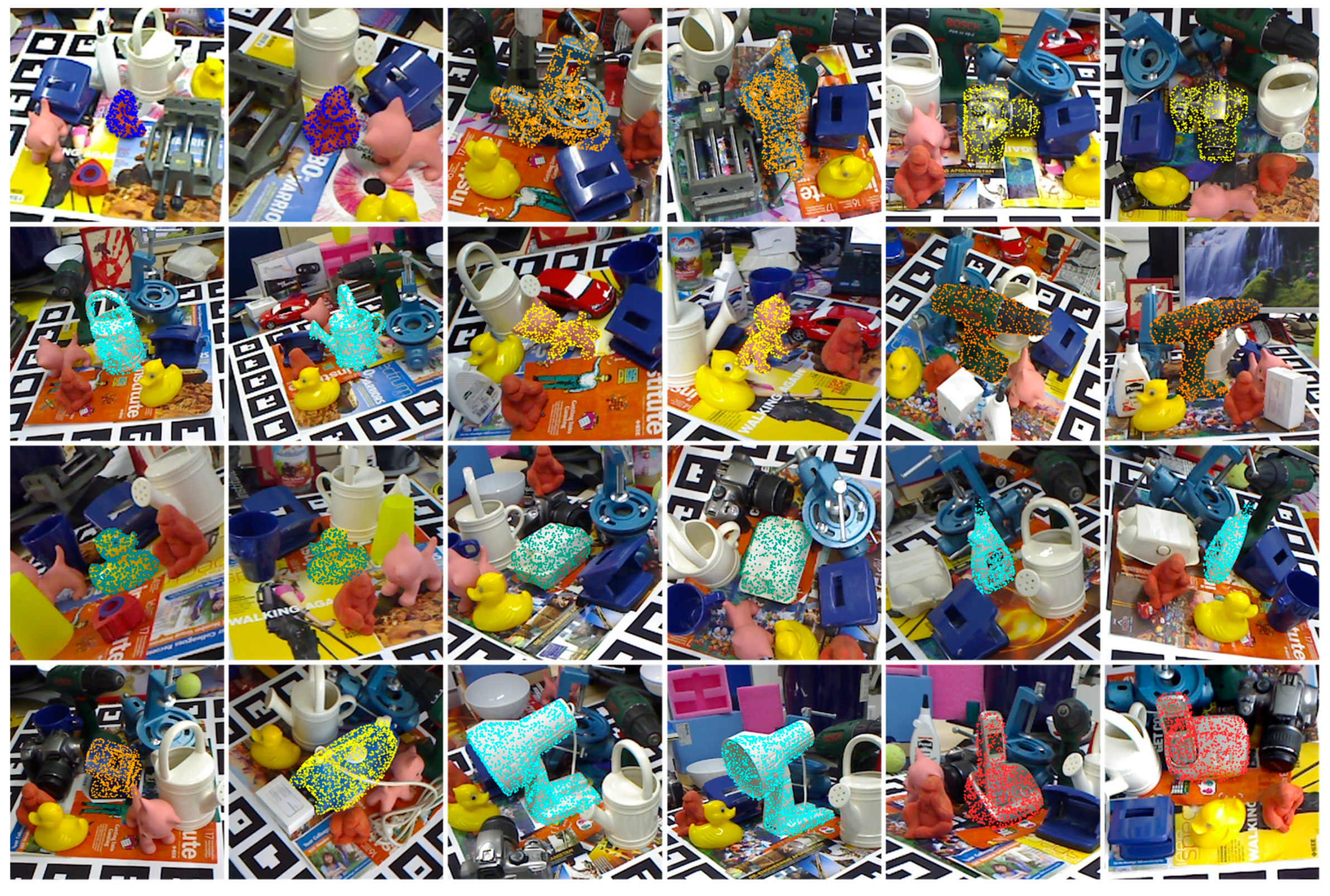
Linemod dataset: The Linemod dataset is a benchmark dataset for object pose estimation. The dataset contains 13 video frame images of weakly textured objects. It has the characteristics of cluttered scenes, illumination variations, and weakly textured objects. It makes the object pose estimation algorithm more challenging on this dataset.
(2)
Occlusion Linemod dataset: The Occlusion Linemod dataset was created by adding annotations to each scene of the Linemod dataset and each image has different degrees of occlusion. Severely occluded object pose estimation is the challenge for this dataset.

4.2. Evaluation Metrics

We employ average distance ADD and ADD-S to evaluate the accuracy of object pose estimation methods. For asymmetric objects, the average distance ADD is used to evaluate. It calculates the average distance between the corresponding point pairs of the target model point cloud in the two states of the real pose [ R * ,   t * ] and the estimated pose [R, t]. ADD is defined as follows:
ADD = 1 N x G ( Rx + t )     ( R * x + t * )
where G represents the point set of the target model point cloud, x represents a point in the point cloud G, N represents the number of points in the point cloud G. For symmetric objects, one state has multiple poses. Therefore, the average distance to the nearest point ADD-S is used as the evaluation index of symmetric objects. ADD-S is defined as follows:
ADD - S = 1 N x 1 G min x 2 G ( Rx 1 + t )     ( R * x 2 + t * )
If the average distance is less than the set threshold, the requirement is considered to be satisfied, otherwise it is not. Usually, the set threshold is 10% of the diameter of the 3D model of the target object.

4.3. Implementation Details

The point cloud is normalized during the dataset loading phase, adding random noise to the image. It is beneficial for the network to learn point cloud and color features, and to increase the robustness of the network. The 32-dimensional point cloud features are outputted through the PointNet network. The point cloud features and the RGB image are spliced along the channel dimension to form a 35-channel image. Feature extraction is performed on the 35-channel image through CNN, and the feature map of size h   ×   w   ×   64 is outputted, combining the 64-channel color features with the point cloud again. Finally, point cloud data of size n   ×   ( 3 + 64 ) is formed. The combined point cloud is then fed into the improved PointNet++ network. The final output is a set of 1664-dimensional center point features. This includes 128-dimensional intermediate local features, 512-dimensional local features outputted by the last abstraction layer and 1024-dimensional global features. Finally, the poses and confidence are regressed to each center point feature vector. The iterative network is composed of three fully connected layers. It predicts the residual pose from the fused global features. Our method uses 2373 images for the Linemod dataset for training and 13,404 images for testing during the training period. For the Occlusion Linemod dataset, 180 images are used for training and 1034 images are used for testing. It was repeated 20 times for each epoch. The pose estimation backbone network is trained first until convergence, and then the iterative network is trained automatically according to the set threshold. The best parameters are obtained after training: the batch size is eight, learning rate is 0.0001, learning rate decay rate is 0.35, the threshold for starting training iterative network is 0.012, the maximum number of epochs for training is 600, and the random noise range is 0.037, the hyperparameter w of the loss function is 0.016, the decay rate of w is 0.37, the decay threshold for learning rate and w is 0.015, and the number of iterations of the iterative network is four.

4.4. Results on the Benchmark Datasets

To evaluate the performance of our algorithm for pose estimation, several sets of experiments are designed and the results are presented below.

4.4.1. Result on the Linemod Dataset

Table 1 shows the results of our method on the Linemod dataset for estimating the pose based on the ADD(-S) evaluation metric. Our method uses ResNet18 + PSPNet network as the image feature extraction network. In this table, the bold indicates the method where the input image is RGB. In the case of using iterative networks, our method achieves the best accuracy of 99.5% on the Linemod dataset, which is 0.1% higher than PVN3D [39], and the accuracy reached 98.1% without using iterative networks. It was 3.8% higher than Densefusion [28], which used an iterative approach, 19.1% higher than SSD6D-ICP [24], and 24.4% higher than PointFusion [42]. It shows that our method outperforms other methods in both feature extraction and feature fusion. Comparing our method using iterative network with PoseCNN [23], PVNet [19], CDPN [15], it is 10.9%, 13.2%, 9.6% higher, respectively. It shows that the depth information of the target object is beneficial to improve the accuracy of object positional estimation. The visualization of the Linemod dataset results is shown in Figure 7. We rotate and pan the point the cloud model and project it onto the RGB image.
The RGBD camera captures images under dark or strong light conditions, which only affects the RGB image and does not affect the depth image. Therefore, in the same scene, we change the luminance value of the RGB image to verify the robustness of the method proposed in this paper under illumination. Figure 8 shows the pose estimation results of our method under the condition of illumination change. It can be seen that our method fuses the features of RGB image and depth image, which can better solve the problem of pose estimation under the condition of illumination change.

4.4.2. Result on the Occlusion Linemod Dataset

Table 2 shows the results of the proposed method on the dataset of Occlusion Linemod using ADD(-S) evaluation metrics. The ResNet18 + PSPNet network was used as the image feature extraction network. Our method achieves an accuracy of 86.8%. It is 5.4% higher than Densefusion [28] and 3.2% higher than ANDC [40]. It shows that our method uses pixel-level fusion features, and regresses the pose for each feature vector, and finally selects the best pose, which can better handle severe occlusion and background clutter. Our method is 8.8% higher than the PoseCNN [23] that uses only RGB images. It shows that in the case of severe occlusion, CNN cannot extract more features from color images. The feature fusion of color images and depth images is needed to effectively solve the problem of object pose estimation under severe occlusion. Our method outperforms Densefusion by 6.2% and 17.3% on two smaller objects, apes and ducks, respectively. It shows that our method can fully integrate color and depth information. Furthermore, intermediate local region features and global features are introduced for each center point feature, which can show better robustness in the case of occlusion. The visualization of the Occlusion Linemod dataset results is shown in Figure 9. Some of them are heavily occluded, however the performance of the proposed method is also excellent.

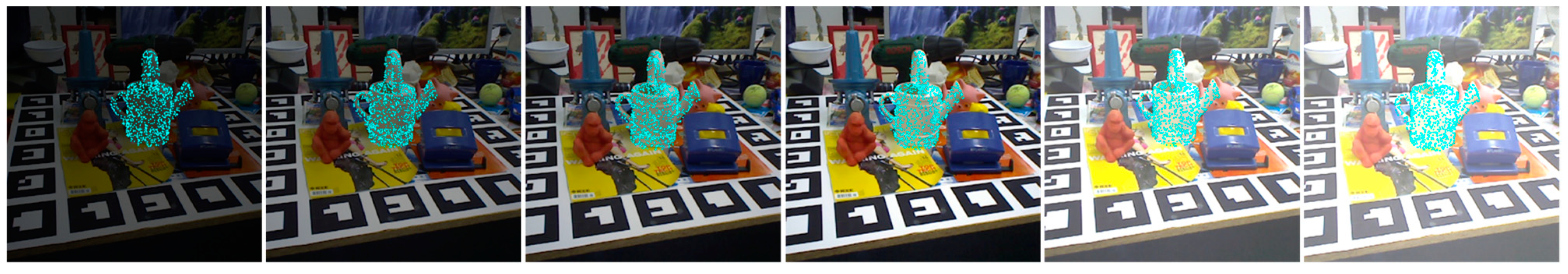
4.4.3. Noise Experiment

When an RGBD camera captures images in a real environment, noise has a greater impact on depth images. The data for each pixel in the depth image is the distance from the object to the camera, in millimeters. Therefore, we add random noise to the depth images of the Linemod dataset to verify the robustness of our pose estimation model to noise. Table 3 shows the performance of our model under increasing random noise. The random noise here is to add random numbers to each pixel of the depth map, and the random number range is (−v, v). Since our model has added random noise to the depth image in the training stage, and regresses the pose for each feature vector, and then selects the pose with the highest confidence as the final result. Therefore, our model can also have good accuracy in the case of random noise in the range of (−30.0, 30.0).

4.5. Ablation Experiments

We performed a series of ablation experiments. The influence of different image feature extraction network structures on the performance of the entire pose estimation network is analyzed.
Table 4 shows the comparison of our method with the Densefusion [28] method under different structures. The first structure is a picture feature extraction network consisting of ResNet18 and PSPNet. In which, ResNet18 is the initial feature extraction and PSPNet performs multi-scale feature extraction. Our method achieves 98.1% and 99.5% with and without the iterative method, respectively, which are both better than Densefusion. To reduce the amount of model parameters and the memory footprint of the model, we integrate depthwise separable convolutions into the network. Therefore, we use MobileNetv2 and PSPNet to form a picture feature extraction network. Our method achieves 98.0% and 99.1% accuracy with and without iterative methods, respectively, which are both better than Densefusion. Experiments show that our two-end feature fusion network can fully fuse color and depth information, and while reducing the amount of network parameters, it can also show good performance.
Table 5 shows the comparison of our model’s memory space, inference speed, model training time, model parameters and Linemod dataset accuracy under different image feature extraction network structures. With the increase in the number of ResNet network layers, the amount of model parameters and the occupied memory space increase sharply, and the inference speed and training speed become slower. However, the pose estimation accuracy did not increase, although when we use MobileNetv2 + PSPNet as the image feature extraction network structure, the memory space of the entire model is 49.3 MB, which is 44.3 MB less than the memory space of using the ResNet18 + PSPNet network structure. In addition, the inference express and training speed are faster, and the number of parameters is reduced. Experiments show that our model can maintain a good accuracy while reducing the number of parameters and occupying memory space. Furthermore, the model parameters are small, which is easy to deploy on mobile devices.

5. Conclusions

In this paper, we propose a lightweight two-end feature fusion network. It is mainly used to estimate the 6D pose of known objects in RGBD images. The method firstly extracts features from the object point cloud. The point cloud features are then used as the geometric supplementary information of the RGB images for pixel-level stitching. Feature extraction is performed on the stitched images. The extracted color features are used as the color supplementary information of the point cloud for point-by-point combination. Then feature extraction is performed on the combined point cloud. Finally, a set of centroid features is obtained by fusing local features and global features, and we then use each center point feature to estimate the object pose. This fusion method can effectively combine depth and color information, as well as show the best performance on two benchmark datasets. Experiments show that our method can accurately estimate the pose of objects under severe occlusion, background clutter, and poor illumination. Our model is also robust to noise, and maintains good performance while reducing the number of model parameters. All in all, our method provides a new idea for the application of object pose estimation methods on mobile devices.

Author Contributions

Conceptualization, L.Z., H.P., L.X. and Z.W.; methodology, L.Z.; software, L.Z.; validation, L.Z. and L.X.; formal analysis, L.X. and Z.W.; investigation, L.Z.; data curation, H.P.; writing—original draft preparation, L.Z.; writing—review and editing, L.Z., H.P., L.X. and Z.W.; visualization, L.Z.; supervision, L.X., and Z.W.; project administration, L.Z. All authors have read and agreed to the published version of the manuscript.

Funding

This research was funded by National Key R&D Program of China (Grant No. 2018YFC2001700) and Beijing Natural Science Foundation (No. L192005).

Institutional Review Board Statement

Not applicable.

Informed Consent Statement

Not applicable.

Data Availability Statement

Not applicable.

Conflicts of Interest

The authors declare no conflict of interest.

References

  1. Bay, H.; Tuytelaars, T.; Gool, L.V. Surf: Speeded up robust features. In Proceedings of the European Conference on Computer Vision, Graz, Austria, 7–13 May 2006. [Google Scholar]
  2. Lowe, D.G. Object recognition from local scale-invariant features. In Proceedings of the Seventh IEEE International Conference on Computer Vision, Kerkyra, Greece, 20–27 September 1999. [Google Scholar]
  3. Rothganger, F.; Lazebnik, S.; Schmid, C.; Ponce, J. 3D object modeling and recognition using local affine-invariant image descriptors and multiview spatial constraints. Int. J. Comput. Vis. 2006, 66, 231–259. [Google Scholar] [CrossRef] [Green Version]
  4. Rublee, E.; Rabaud, V.; Konolige, K.; Bradski, G. ORB: An efficient alternative to SIFT or SURF. In Proceedings of the 2011 International Conference on Computer Vision, Barcelona, Spain, 6–13 November 2011. [Google Scholar]
  5. Ng, P.C.; Henikoff, S. SIFT: Predicting amino acid changes that affect protein function. Nucleic Acids Res. 2003, 31, 3812–3814. [Google Scholar] [CrossRef] [PubMed] [Green Version]
  6. Hinterstoisser, S.; Lepetit, V.; Ilic, S.; Holzer, S.; Bradski, G.; Konolige, K.; Navab, N. Model based training, detection and pose estimation of texture-less 3d objects in heavily cluttered scenes. In Proceedings of the Asian Conference on Computer Vision, Daejeon, Korea, 5–9 November 2012. [Google Scholar]
  7. Rios-Cabrera, R.; Tuytelaars, T. Discriminatively Trained Templates for 3D Object Detection: A Real Time Scalable Approach. In Proceedings of the 2013 IEEE International Conference on Computer Vision, Sydney, NSW, Australia, 1–8 December 2013. [Google Scholar]
  8. Hinterstoisser, S.; Cagniart, C.; Ilic, S.; Sturm, P.; Navab, N.; Fua, P.; Lepetit, V. Gradient Response Maps for Real-Time Detection of Textureless Objects. IEEE Trans. Pattern Anal. Mach. Intell. 2011, 34, 876–888. [Google Scholar] [CrossRef] [PubMed] [Green Version]
  9. Sundermeyer, M.; Marton, Z.C.; Durner, M.; Brucker, M.; Triebel, R. Implicit 3D Orientation Learning for 6D Object Detection from RGB Images. In Proceedings of the European Conference on Computer Vision, Munich, Germany, 8–14 September 2018. [Google Scholar]
  10. Zhu, M.; Derpanis, K.G.; Yang, Y.; Brahmbhatt, S.; Zhang, M.; Phillips, C.; Lecce, M.; Daniilidis, K. Single image 3D object detection and pose estimation for grasping. In Proceedings of the 2014 IEEE International Conference on Robotics and Automation (ICRA), Hong Kong, China, 31 May–7 June 2014. [Google Scholar]
  11. Lepetit, V.; Moreno-Noguer, F.; Fua, P. Epnp: An accurate o (n) solution to the pnp problem. Int. J. Comput. Vis. 2009, 81, 155–166. [Google Scholar] [CrossRef] [Green Version]
  12. Tian, Y.; Yang, G.; Wang, Z.; Wang, H.; Liang, Z. Apple detection during different growth stages in orchards using the improved YOLO-V3 model. Comput. Electron. Agric. 2019, 157, 417–426. [Google Scholar] [CrossRef]
  13. He, K.; Zhang, X.; Ren, S.; Sun, J. Deep residual learning for image recognition. In Proceedings of the IEEE Conference on Computer Vision and Pattern Recognition, Las Vegas, NV, USA, 26 June–1 July 2016. [Google Scholar]
  14. Pavlakos, G.; Zhou, X.; Chan, A.; Derpanis, K.G.; Daniilidis, K. 6-DoF object pose from semantic keypoints. In Proceedings of the 2017 IEEE International Conference on Robotics and Automation (ICRA), Singapore, 29 May–3 June 2017. [Google Scholar]
  15. Li, Z.; Wang, G.; Ji, X. CDPN: Coordinates-Based Disentangled Pose Network for Real-Time RGB-Based 6-DoF Object Pose Estimation. In Proceedings of the 2019 IEEE/CVF International Conference on Computer Vision (ICCV), Seoul, Korea, 27 October–2 November 2019. [Google Scholar]
  16. Tekin, B.; Sinha, S.N.; Fua, P. Real-Time Seamless Single Shot 6D Object Pose Prediction. In Proceedings of the 2018 IEEE/CVF Conference on Computer Vision and Pattern Recognition, Salt Lake City, UT, USA, 18–23 June 2018. [Google Scholar]
  17. Zakharov, S.; Shugurov, I.; Ilic, S. DPOD: 6D Pose Object Detector and Refiner. In Proceedings of the 2019 IEEE/CVF International Conference on Computer Vision (ICCV), Seoul, Korea, 27 October–2 November 2019. [Google Scholar]
  18. Hu, Y.; Hugonot, J.; Fua, P.; Salzmann, M. Segmentation-Driven 6D Object Pose Estimation. In Proceedings of the 2019 IEEE/CVF Conference on Computer Vision and Pattern Recognition (CVPR), Long Beach, CA, USA, 15–20 June 2019. [Google Scholar]
  19. Peng, S.; Liu, Y.; Huang, Q.; Zhou, X.; Bao, H. PVNet: Pixel-wise Voting Network for 6DoF Object Pose Estimation. In Proceedings of the 2019 IEEE/CVF Conference on Computer Vision and Pattern Recognition (CVPR), Long Beach, CA, USA, 15–20 June 2019. [Google Scholar]
  20. Song, C.; Song, J.; Huang, Q. HybridPose: 6D Object Pose Estimation Under Hybrid Representations. In Proceedings of the 2020 IEEE/CVF Conference on Computer Vision and Pattern Recognition (CVPR), Seattle, WA, USA, 13–19 June 2020. [Google Scholar]
  21. Tremblay, J.; To, T.; Sundaralingam, B.; Xiang, Y.; Fox, D.; Birchfield, S. Deep object pose estimation for semantic robotic grasping of household objects. In Proceedings of the 2018 Conference on Robot Learning (CoRL), Zürich, Switzerland, 29–31 October 2018. [Google Scholar]
  22. Kendall, A.; Grimes, M.; Cipolla, R. PoseNet: A Convolutional Network for Real-Time 6-DOF Camera Relocalization. In Proceedings of the 2015 IEEE International Conference on Computer Vision (ICCV), Santiago, Chile, 7–13 December 2015. [Google Scholar]
  23. Xiang, Y.; Schmidt, T.; Narayanan, V.; Fox, D. PoseCNN: A Convolutional Neural Network for 6D Object Pose Estimation in Cluttered Scenes. arXiv 2017, arXiv:1711.00199. [Google Scholar]
  24. Kehl, W.; Manhardt, F.; Tombari, F.; Ilic, S.; Navab, N. SSD-6D: Making RGB-Based 3D Detection and 6D Pose Estimation Great Again. In Proceedings of the 2017 IEEE International Conference on Computer Vision (ICCV), Venice, Italy, 22–29 October 2017. [Google Scholar]
  25. Rusinkiewicz, S.; Levoy, M. Efficient variants of the ICP algorithm. In Proceedings of the Third International Conference on 3-D Digital Imaging and Modeling, Quebec City, QC, Canada, 28 May–1 June 2001. [Google Scholar]
  26. Romero-Ramire, F.J.; Muñoz-Salinas, R.; Medina-Carnicer, R. Fractal Markers: A New Approach for Long-Range Marker Pose Estimation Under Occlusion. IEEE Access 2019, 7, 169908–169919. [Google Scholar] [CrossRef]
  27. Hu, P.; Kaashki, N.N.; Dadarlat, V.; Munteanu, A. Learning to Estimate the Body Shape Under Clothing from a Single 3-D Scan. IEEE Trans. Ind. Inform. 2021, 17, 3793–3802. [Google Scholar] [CrossRef]
  28. Wang, C.; Xu, D.; Zhu, Y.; Martín-Martín, R.; Lu, C.; Fei-Fei, L.; Savarese, S. DenseFusion: 6D Object Pose Estimation by Iterative Dense Fusion. In Proceedings of the 2019 IEEE/CVF Conference on Computer Vision and Pattern Recognition (CVPR), Long Beach, CA, USA, 15–20 June 2019. [Google Scholar]
  29. Charles, R.Q.; Su, H.; Kaichun, M.; Guibas, L.J. PointNet: Deep Learning on Point Sets for 3D Classification and Segmentation. In Proceedings of the 2017 IEEE Conference on Computer Vision and Pattern Recognition (CVPR), Honolulu, HI, USA, 21–26 July 2017. [Google Scholar]
  30. Qi, C.R.; Li, Y.; Hao, S.; Guibas, L.J. PointNet++: Deep Hierarchical Feature Learning on Point Sets in a Metric Space. arXiv 2017, arXiv:1706.02413. [Google Scholar]
  31. Wohlhart, P.; Lepetit, V. Learning descriptors for object recognition and 3D pose estimation. In Proceedings of the 2015 IEEE Conference on Computer Vision and Pattern Recognition (CVPR), Boston, MA, USA, 7–12 June 2015. [Google Scholar]
  32. Brachmann, E.; Krull, A.; Michel, F.; Gumhold, S.; Shotton, J.; Rother, C. Learning 6D Object Pose Estimation Using 3D Object Coordinates. In Proceedings of the European Conference on Computer Vision, Zurich, Switzerland, 6–12 September 2014. [Google Scholar]
  33. Kehl, W.; Milletari, F.; Tombari, F.; Ilic, S.; Navab, N. Deep learning of local RGB-D patches for 3D object detection and 6D pose estimation. In Proceedings of the European Conference on Computer Vision, Amsterdam, The Netherlands, 11–14 October 2016. [Google Scholar]
  34. Tejani, A.; Tang, D.; Kouskouridas, R.; Kim, T.-K. Latent-class hough forests for 3D object detection and pose estimation. In Proceedings of the European Conference on Computer Vision, Zurich, Switzerland, 6–12 September 2014. [Google Scholar]
  35. Drost, B.; Ulrich, M.; Navab, N.; Ilic, S. Model globally, match locally: Efficient and robust 3D object recognition. In Proceedings of the 2010 IEEE Computer Society Conference on Computer Vision and Pattern Recognition, San Francisco, CA, USA, 13–18 June 2010. [Google Scholar]
  36. Li, C.; Bai, J.; Hager, G.D. A unified framework for multi-view multi-class object pose estimation. In Proceedings of the European Conference on Computer Vision, Munich, Germany, 8–14 September 2018. [Google Scholar]
  37. Tulsiani, S.; Malik, J. Viewpoints and keypoints. In Proceedings of the 2015 IEEE Conference on Computer Vision and Pattern Recognition (CVPR), Boston, MA, USA, 7–12 June 2015. [Google Scholar]
  38. Mousavian, A.; Anguelov, D.; Flynn, J.; Košecká, J. 3D Bounding Box Estimation Using Deep Learning and Geometry. In Proceedings of the 2017 IEEE Conference on Computer Vision and Pattern Recognition (CVPR), Honolulu, HI, USA, 21–26 July 2017. [Google Scholar]
  39. He, Y.; Sun, W.; Huang, H.; Liu, J.; Fan, H.; Sun, J. PVN3D: A Deep Point-Wise 3D Keypoints Voting Network for 6DoF Pose Estimation. In Proceedings of the 2020 IEEE/CVF Conference on Computer Vision and Pattern Recognition (CVPR), Seattle, WA, USA, 13–19 June 2020. [Google Scholar]
  40. Zhou, G.; Yan, Y.; Wang, D.; Chen, Q. A Novel Depth and Color Feature Fusion Framework for 6D Object Pose Estimation. IEEE Trans Multimed. 2020, 23, 1630–1639. [Google Scholar] [CrossRef]
  41. Wada, K.; Sucar, E.; James, S.; Lenton, D.; Davison, A.J. MoreFusion: Multi-object Reasoning for 6D Pose Estimation from Volumetric Fusion. In Proceedings of the 2020 IEEE/CVF Conference on Computer Vision and Pattern Recognition (CVPR), Seattle, WA, USA, 13–19 June 2020. [Google Scholar]
  42. Xu, D.; Anguelov, D.; Jain, A. PointFusion: Deep Sensor Fusion for 3D Bounding Box Estimation. In Proceedings of the 2018 IEEE/CVF Conference on Computer Vision and Pattern Recognition, Salt Lake City, UT, USA, 18–23 June 2018. [Google Scholar]
  43. Qi, C.R.; Liu, W.; Wu, C.; Su, H.; Guibas, J.L. Frustum PointNets for 3D Object Detection from RGB-D Data. In Proceedings of the 2018 IEEE/CVF Conference on Computer Vision and Pattern Recognition, Salt Lake City, UT, USA, 18–23 June 2018. [Google Scholar]
  44. Li, Y.; Qi, H.; Dai, J.; Wei, Y. Fully convolutional instance-aware semantic segmentation. In Proceedings of the 2017 IEEE Conference on Computer Vision and Pattern Recognition (CVPR), Honolulu, HI, USA, 21–26 July 2017. [Google Scholar]
  45. Zhao, H.; Shi, J.; Qi, X.; Wang, X.; Jia, J. Pyramid Scene Parsing Network. In Proceedings of the 2017 IEEE Conference on Computer Vision and Pattern Recognition (CVPR), Honolulu, HI, USA, 21–26 July 2017. [Google Scholar]
  46. Sandler, M.; Howard, A.; Zhu, M.; Zhmoginov, A.; Chen, L.C. MobileNetV2: Inverted Residuals and Linear Bottlenecks. In Proceedings of the 2018 IEEE/CVF Conference on Computer Vision and Pattern Recognition, Salt Lake City, UT, USA, 18–23 June 2018. [Google Scholar]
Figure 1. Our algorithm framework. First, the depth image and RGB image of the target object are obtained by semantic segmentation, and the depth map is converted into a point cloud. Secondly, feature extraction is performed on the point cloud, feature fusion of the point cloud features with the color image, feature extraction of the fused image, and feature fusion of the extracted features with the point cloud again. Finally, the obtained set of centroid features are regressed on the object 6D poses, and the poses with the highest confidence are selected as the final results. (For simplicity, the pose iteration network is not described here).
Machines 10 00254 g001
Figure 2. Structure diagram of the image feature extraction network. We use ResNet for preliminary feature extraction of color images, and apply PSPNet for multi-scale feature extraction. Finally, the upsampling module is used to keep the output size unchanged.
Machines 10 00254 g002
Figure 3. Improved PointNet++ point cloud feature extraction network structure.
Machines 10 00254 g003
Figure 4. Pose iterative network. The predicted residual pose transforms the input point cloud.
Machines 10 00254 g004
Figure 5. Schematic diagram of the pose iteration network. The point cloud is transformed according to the predicted pose and the residual pose.
Machines 10 00254 g005
Figure 6. Schematic diagram of the calculation process of depthwise separable convolution.
Machines 10 00254 g006
Figure 7. Visualization of the Linemod dataset results, where we rotate and translate the point cloud model and project it on the image.
Machines 10 00254 g007
Figure 8. Pose estimation results under conditions of varying illumination, where we projected the point cloud model onto the image after rotation and translation.
Machines 10 00254 g008
Figure 9. Visualization of the results of the Occlusion Linemod dataset, where we projected the point cloud model on the image after rotation and translation.
Machines 10 00254 g009
Table 1. The accuracy of our method according to the ADD(-S) metric on the Linemod dataset compared to the benchmark method. Where per stands for per-pixel and iter stands for iterative.
PoseCNNPVNetCDPNSSD6D-
ICP
Point-
Fusion
Dense-
Fusion
PVN3DOurs (per)Ours (iter)
ape77.043.664.465.070.492.397.395.199.0
benchvise97.599.997.880.080.793.299.797.599.9
camera93.586.991.778.060.894.499.699.099.1
can96.595.595.986.061.193.199.597.498.7
cat82.179.383.870.079.196.599.898.699.6
driller95.096.496.273.047.387.099.397.1100.0
duck77.752.666.866.063.092.398.297.599.2
eggbox97.199.299.7100.099.999.899.899.9100.0
glue99.495.799.6100.099.3100.0100.099.8100.0
holepuncher52.882.085.849.071.892.199.998.099.4
iron98.398.997.978.083.297.099.798.999.3
lamp97.599.397.973.062.395.399.897.899.9
phone87.792.490.879.078.892.899.598.599.4
average88.686.389.979.073.794.399.498.199.5
Table 2. The accuracy of our method is compared with the benchmark method on the Occlusion Linemod dataset according to the ADD(-S) metric.
PVNetHinterstoisserMichelPoseCNNDensefusionANDCOurs
ape15.881.480.776.273.268.479.4
can63.394.788.587.488.692.689.7
cat16.655.257.852.272.277.980.7
driller65.686.094.790.392.595.194.4
duck25.279.774.477.759.662.176.9
eggbox50.165.547.672.294.296.096.9
glue49.652.173.876.792.693.595.5
holepuncher39.695.596.391.478.783.680.8
average40.776.376.778.081.483.686.8
Table 3. Accuracy contrasts of our method under increasing random noise.
Noise Range (mm)0.05.010.015.020.025.030.0
Accuracy99.5%99.5%99.4%99.3%99.2%99.1%99.1%
Table 4. Accuracy comparison of ADD(-S) metrics on Linemod dataset using different image feature extraction networks. Where rs stands for ResNet18, mo stands for MobileNetv2, per stands for per-pixel, and iter stands for iterative.
Densefusion
(per-Pixel)
Densefusin
(Iterative)
Ours (per-rs)Ours (per-mo)Ours (iter-rs)Ours (iter-mo)
ape79.592.395.195.699.098.0
benchvise84.293.297.597.699.999.1
camera76.594.499.098.999.198.9
can86.693.197.497.298.798.7
cat88.896.598.698.699.699.4
driller77.787.097.197.0100.099.3
duck76.392.397.597.499.299.1
eggbox99.999.899.999.8100.099.4
glue99.4100.099.899.8100.099.5
holepuncher79.092.198.097.699.498.9
iron92.197.098.999.099.399.4
lamp92.395.397.897.899.999.6
phone88.092.898.598.499.499.2
average86.294.398.198.099.599.1
Table 5. Comparison of different color feature extraction network structures on the Linemod dataset in terms of model memory usage, inference speed, training time, model parameter quantity, and accuracy.
ResNet152 +
PSPNet
ResNet101 +
PSPNet
ResNet50 +
PSPNet
ResNet34 + PSPNetResNet18 + PSPNetMobileNetV2 + PSPNet
Space(MB)376313.6237.8133.993.649.3
Run-time(ms/frame)2431611209175 45
Train-time(h/epoch)3.12.52.11.090.650.35
Parameter184,111,680152,916,544115,036,73663,083,07242,900,41624,542,336
Accuracy99.5%99.5%99.5%99.4%99.5%99.1%
Publisher’s Note: MDPI stays neutral with regard to jurisdictional claims in published maps and institutional affiliations.

