A Novel Experimental Method for Identifying the Flux Linkage Map of a High-Power Medium-Voltage Electrically Excited Synchronous Machine with Double Stator Winding

Abstract

Accurate knowledge of the magnitude and position of the magnetic flux is essential for implementing field-oriented control (FOC) and achieving high-performance behaviour of AC drives. For estimating the flux in a wide range of speeds, so-called hybrid flux estimators, which are a combination of current-model and voltage-model based estimators, are usually used. Since the inductances are used as parameters in the current model, knowledge of the actual flux–current relationship, i.e., of the actual flux linkage map, is inevitable. In this paper, a novel experimental method for identifying the flux linkage map of an electrically excited synchronous machine (EESM) with double stator winding is proposed, which, unlike most existing experimental methods, does not require an additional machine to be used as a load. The flux is determined for different operating points to which the unloaded and sped-up machine is brought to by injecting d- and q-axis stator current components, whereby the current controllers are used to keep them constant for a certain operating point. The proposed method has been used to identify the flux linkage map of a medium-voltage EESM with double stator winding. A more than acceptable accuracy confirmed by comparison with three different analytical methods, together with the fact that it does not require a complex experimental setup, makes the proposed method suitable for the identification of a machine’s flux linkage map in an industrial environment.

1. Introduction

Electrically excited synchronous machines (EESMs) are mainly associated with power generation. However, due to numerous advantages over other types of machines such as high efficiency in a wide range of speeds, high power density and reactive power control capability, EESM are being increasingly used in variable speed drives for high-power application such as in rolling mills, mine hoists, pumps, compressors and ship propulsion [1,2,3]. At the same time, high-performance dynamic behavior of an EESM can be achieved by applying the so-called field-oriented control (FOC) principle. The FOC of an EESM is based on representing the space vector of the stator current in a rotating reference frame whose real axis is aligned with the space vector of the magnetizing (air gap) flux. In such a reference frame, the space vector of the stator current can be decomposed into a flux-producing and torque-producing component, thus allowing decoupled control of the machine’s flux and torque. In addition, the existence of the field winding or, more precisely, the possibility of controlling the field current allows the design of control schemes for achieving unity power factor operation, thus minimizing both machine and inverter sizing and losses [4,5].

The implementation of the FOC requires knowledge of both the magnitude and position of the space vector of the magnetic flux used for orientation, hence accurate estimation of the flux is essential for achieving high-performance control. However, flux estimation is not an easy task since it requires knowledge of machine’s equivalent circuit parameters, especially the inductances which can vary significantly depending on the operating point of the machine [6]. Although there are many different methods for estimating the flux, in essence the flux can be determined in two ways [7]. The first approach is to estimate the flux based on the measured currents and the known flux–current relationship, i.e., the so-called current model of the machine. The other approach is to estimate the flux based on the so-called voltage model of the machine, i.e., by integrating the back electromotive force (EMF) that can be calculated using the measured (or reconstructed) voltage and measured currents. Unfortunately, although they do not require much computational effort, which makes them very easy for practical implementation, both the current model- and the voltage model-based flux estimation method have some limitations in certain operating regions.

Since the flux and the current are linked via the inductances, the fact that inductance values may vary with the operating point (or more precisely with the load) is a major problem for flux estimation based on the machine’s current model [8,9]. Moreover, due to the influence of magnetic saturation and cross-coupling phenomena, the dependency of the inductance values on the currents becomes highly nonlinear [10,11,12]. Therefore, in order to accurately estimate the flux, it is necessary to know the functional dependence between the inductances and currents. Basically, the machine’s inductances can be determined using finite element method (FEM) simulations [6,13,14,15] or experimentally [6]. However, these methods are not easy to conduct. For example, if the inductances are determined using FEM simulation, it is necessary to know the exact geometry, i.e., the construction of the machine. If, on the other hand, the inductances are determined experimentally, the machine on which the measurement is performed has to be loaded, and the measurement itself needs to be performed several times in order to cover the desired range of the magnetizing current values. This is, of course, difficult to do outside the laboratory environment, especially for high-power machines because it would require another machine of at least the same amount of power to act as a load.

Although the voltage model-based flux estimation is much less sensitive to parameter variation due to the fact that it requires only the knowledge of the stator resistance (and possibly the stator leakage inductance), it has two main drawbacks [16]. The first problem regarding the voltage model-based estimation stems from the fact that the integrator is prone to drift in case of DC components in the measured signals which can lead to the saturation of the integrator [17] or even to occurrence of torque and speed oscillations, as reported in [18]. The other problem is the inability of accurately calculating the back EMF at low speeds where, due to the low stator voltage, inverter nonlinearities come to fore [18], as well as the influence of resistance variations [19] which become even more prominent if the machine draws high current while operating at low speed.

In order to overcome the drawbacks of conventional flux estimation techniques, a multitude of hybrid method has been proposed in which various combinations of current and voltage models seek to estimate the flux as accurately as possible over the entire speed range, [5,20,21,22,23]. However, knowledge of the actual relationship between the flux and the currents, i.e., of the actual flux linkage map, remains a major obstacle for accurate flux estimation. To accurately determine the flux linkage map of a machine, several experimental methods have been proposed, among which the constant speed [24,25], variable speed [26,27] and signal injection [28,29] methods should be highlighted.

In both constant and variable speed methods, the direct (d) and quadrature (q) axis stator current components are injected into the machine and kept constant, resulting in a constant flux which is then calculated from the steady-state stator voltage equations based on the known speed and the current and voltage measurements. In order to obtain the complete flux linkage map, the calculation of the flux is completed for different combinations of stator current component values, i.e., for different operating points of the machine. Although the problem related to the presence of higher harmonics in the measured signals can be successfully solved (e.g., by applying the Fast Fourier Transform as done in [25]), eliminating the influence of possible resistance variations on calculation of the flux is not trivial. In [24], the authors manage to eliminate the influence of the resistance by calculating the flux as the mean of the flux obtained in the motoring and generating mode. However, the described approach is, as pointed out by the authors, possible only if the other losses in the machine (e.g., iron losses) are negligible. This can, however, be achieved by an appropriate choice of the machine’s speed. The main drawback of most constant and variable speed methods is the complexity of the experimental setup required to perform them or, more precisely, the need for an additional machine. In [26], a flux linkage map identification method has been proposed that does not require an additional machine to be used as a load. Like in other constant or variable speed methods, the identification of the flux linkage map is done by injecting the d- and q-axis stator current components into the machine, whereas an approach similar to the one proposed in [24] was used to eliminate the influence of the resistance on the flux calculation. The influence of resistance and the problem of reconstructing the stator voltage due to the nonlinearities of the inverter have been successfully overcome in [27] where for each operating point two sets of measurements have been performed at constant values of the stator current components and variable speed. Based on these two sets of measurements, voltage equations have been written, and then the influence of the resistance and inverter nonlinearities has been eliminated by algebraic manipulations and the application of an optimization algorithm. Although the proposed method proved to be very effective in determining the flux linkage map, the variable speed was achieved by using an additional machine. In [29], a method has been proposed according to which, under locked rotor, the current in one of the two axes (either d- or q-axis) is kept constant while the other axis is excited by voltage pulses. Unlike aforementioned methods in which the flux is calculated based on algebraic expressions, in this method the flux is obtained by directly integrating the voltage which makes it very sensitive to the occurrence of DC offsets. In [28] a method for the identification of the flux linkage map was proposed which is also based on injecting d- and q-axis stator current components into the machine, but, unlike other methods, these injected currents do not only contain a DC component but also a low-frequency AC component. The change in the saturation level, i.e., the change of machine’s operating point, is achieved by changing the value of the DC component of the injected currents, whereas the presence of the AC component causes the appearance of an AC component in the voltages. Based on the AC current and voltage components, the equivalent impedance of the machine is calculated, as well as the incremental inductances. The flux linkage map of the machine is finally obtained by integrating the calculated incremental inductances.

Although previously described experimental methods ensure accurate identification of the machine’s flux linkage map, performing them requires a rather complex experimental setup which, in most cases, is not available in an industrial environment. On the other hand, performing FEM simulations, as said, requires knowledge of the detailed construction of the machine. Hence, due to the limitations in wider application of FEM simulations and previously described experimental methods, analytical methods [7,8,30,31,32] are usually used to determine the flux linkage map of a machine. However, these analytical methods can be treated as approximate methods since the calculation of the entire flux linkage map is based only on the magnetization curves in the d- and q-axis. Therefore, their accuracy in the whole operating region of the machine is questionable.

This paper presents a novel experimental method for the identification of the flux linkage map of a high-power medium-voltage EESM with double stator winding. The method proposed in this paper does not require the existence of an additional machine to be used as a load, which makes it suitable for determining the EESM’s flux linkage map in an industrial environment, e.g., during drive commissioning. The proposed method can be summarized as follows. The machine is first accelerated to the nominal speed after which the d- and q-axis stator currents are injected. Meanwhile, the field current is set to zero in order to minimize the developed torque of the machine, and thus the change of speed during the identification process. Finally, the flux is calculated based on the fundamental components of the stator currents and voltages obtained by applying the Fourier series analysis to the currents and voltages measured at the machine terminals. The proposed method was experimentally verified on a 14 MW EESM drive. Due to the impossibility of conducting other experimental methods and making a detailed model of the machine required to perform FEM simulations, the proposed method is compared with three commonly used analytical methods [7,31,32] for determining the machine’s flux linkage map.

The rest of the paper is organized as follows. In Section 2, the mathematical model of an EESM with double stator winding is given. Section 3 briefly describes three analytical methods for determining the flux linkage map based on magnetization curves, as these methods are commonly found in the existing literature. The novel experimental method for flux linkage map identification is described in Section 4, and the experimental results, as well as a comparison of the proposed experimental method with existing analytical ones, are given in Section 5. Finally, concluding remarks are given in Section 6.

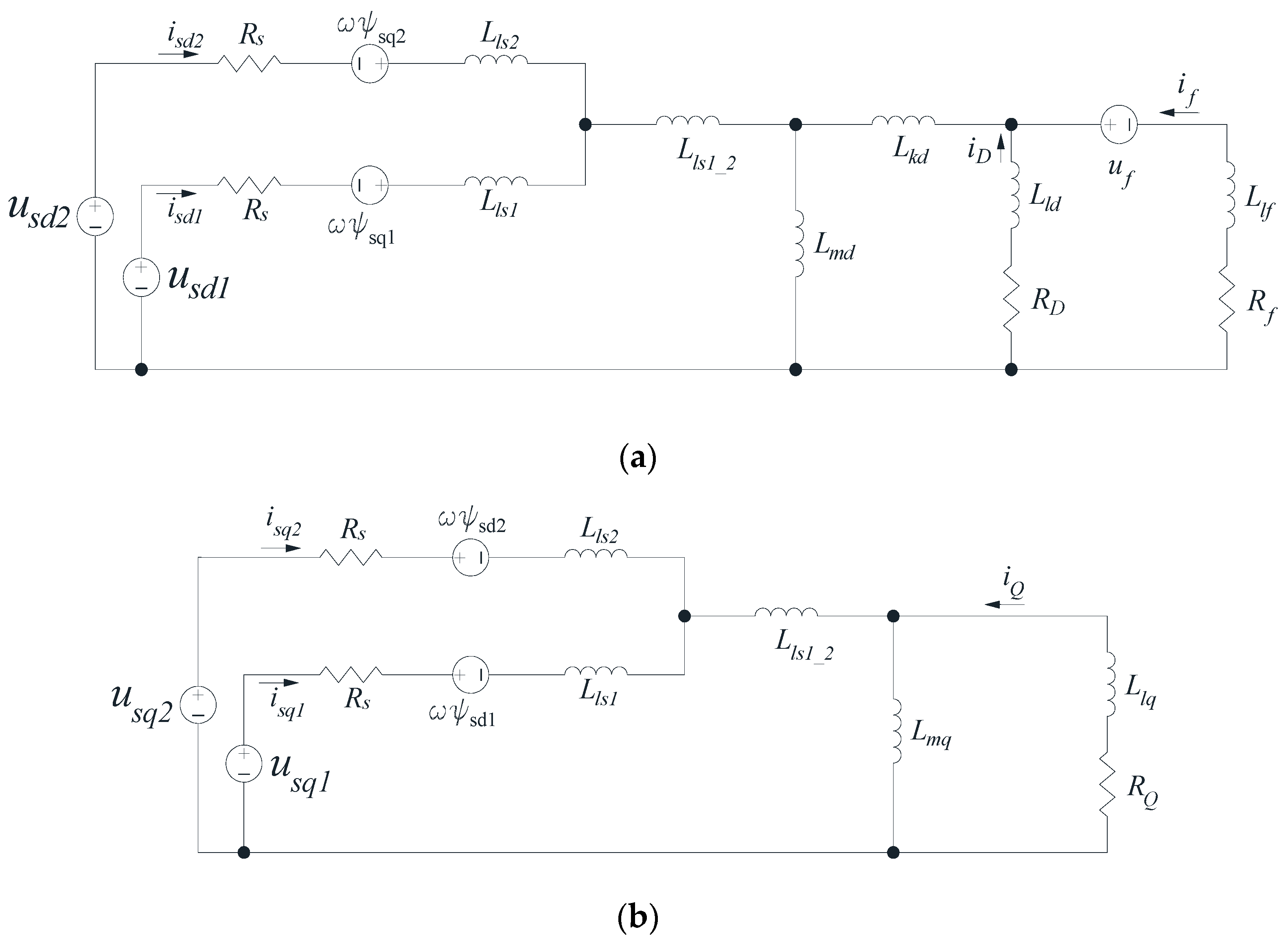
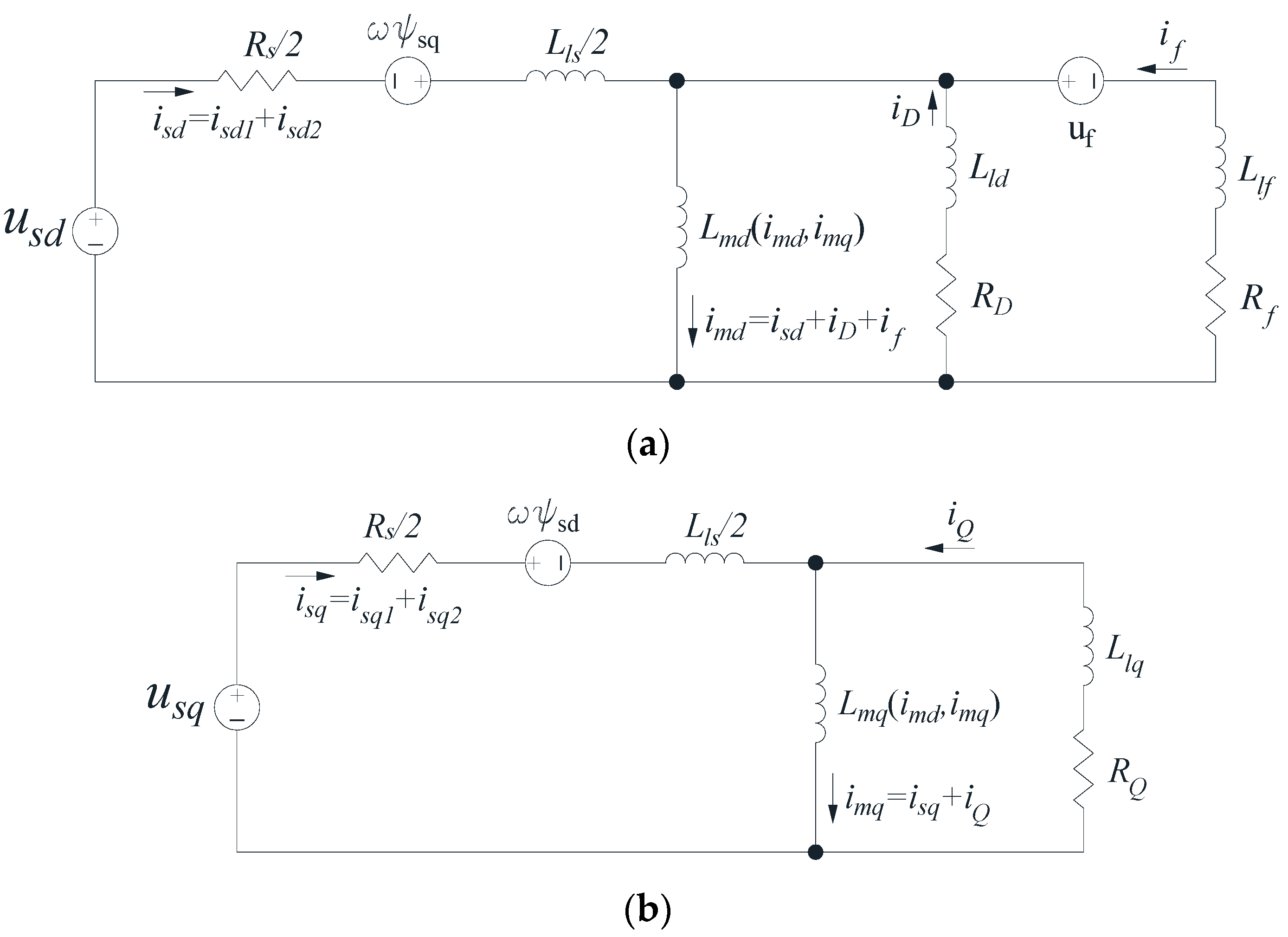
2. Mathematical Model of an EESM with Double Stator Winding

As stated in the introduction, the components of the magnetic flux can be easily calculated from the stator voltage equation in the dq reference frame under the assumption of a constant flux. The equivalent circuits for the d- and q-axis of an EESM with double stator winding are shown in Figure 1 [33], where the meaning of each parameter is given in the description of the figure.

Since we shall consider a machine in which there is no phase shift between the stator windings (YY0 connection), it is possible to assume the following equalities:

$$\begin{array}{l}{u}_{sd1}=u_{sd2}=u_{sd},\\ u_{sq1}=u_{sq2}=u_{sq},\\ L_{ls1\_2}=0,\\ L_{ls1}=L_{ls2}=L_{ls},\\ L_{kd}=0.\end{array}$$

(1)

It follows from Equation (1) that the equivalent circuits shown in Figure 1 can be simplified, which, in the case of the considered EESM with double star-connected stator winding, results in the equivalence circuits shown in Figure 2.

By comparing Figure 1 and Figure 2, one can conclude that the considered machine with double stator winding can be reduced to an equivalent standard machine with a single stator winding. Based on the simplified equivalent circuits shown in Figure 2, the voltage equations of the EESM with double stator winding can be written as:

$$\begin{array}{l}{u}_{sd}=\frac{R_s}{2}{i}_{sd}+\frac{d{\psi }_{sd}}{dt}-\omega {\psi }_{sq},\\ u_{sq}=\frac{R_s}{2}{i}_{sq}+\frac{d{\psi }_{sq}}{dt}+\omega {\psi }_{sd},\\ 0=R_D{i}_D+\frac{d{\psi }_D}{dt},\\ 0=R_Q{i}_Q+\frac{d{\psi }_Q}{dt},\\ u_f=R_f{i}_f+\frac{d{\psi }_f}{dt},\end{array}$$

(2)

with the flux–current relationships being:

$$\begin{array}{l}{\psi }_{sd}=\frac{L_{ls}}{2}{i}_{sd}+L_{md}\left(i_{md},i_{mq}\right)\left(i_{sd}+i_D+i_f\right)=\frac{L_{ls}}{2}{i}_{sd}+L_{md}\left(i_{md},i_{mq}\right)i_{md},\\ {\psi }_{sq}=\frac{L_{ls}}{2}{i}_{sq}+L_{mq}\left(i_{md},i_{mq}\right)\left(i_{sq}+i_Q\right)=\frac{L_{ls}}{2}{i}_{sq}+L_{mq}\left(i_{md},i_{mq}\right)i_{mq},\\ {\psi }_D=L_{lD}{i}_D+L_{md}\left(i_{md},i_{mq}\right)i_{md},\\ {\psi }_Q=L_{lQ}{i}_Q+L_{mq}\left(i_{md},i_{mq}\right)i_{mq,}\\ {\psi }_f=L_{lf}{i}_f+L_{md}\left(i_{md},i_{mq}\right)i_{md},\end{array}$$

(3)

where i_md and i_mq are the d- and q-axis magnetizing current components, respectively. From Equation (3) it can be seen that the magnetizing inductances L_md and L_mq are nonlinearly dependent on the magnetizing currents due to the saturation and cross-saturation effect. Therefore, the following expression can be written for the magnetizing inductances:

$$\begin{array}{l}{\psi }_{md}\left(i_{md},i_{mq}\right)=L_{md}\left(i_{md},i_{mq}\right)i_{md}={\psi }_{sd}\left(i_{md},i_{mq}\right)-\frac{L_{ls}}{2}{i}_{sd},\\ {\psi }_{mq}\left(i_{md},i_{mq}\right)=L_{mq}\left(i_{md},i_{mq}\right)i_{mq}={\psi }_{sq}\left(i_{md},i_{mq}\right)-\frac{L_{ls}}{2}{i}_{sq}.\end{array}$$

(4)

If the flux is assumed to be constant, the time derivatives of its components vanish from the stator voltage Equation (2), hence the magnetizing flux components can be calculated based on the following algebraic equations:

$$\begin{array}{l}{\psi }_{md}=\frac{u_{sq}-\left(R_s/2\right)i_{sq}}{\omega }-\frac{L_{ls}}{2}{i}_{sd},\\ {\psi }_{mq}=\frac{u_{sd}-\left(R_s/2\right)i_{sd}}{-\omega }-\frac{L_{ls}}{2}{i}_{sq}.\end{array}$$

(5)

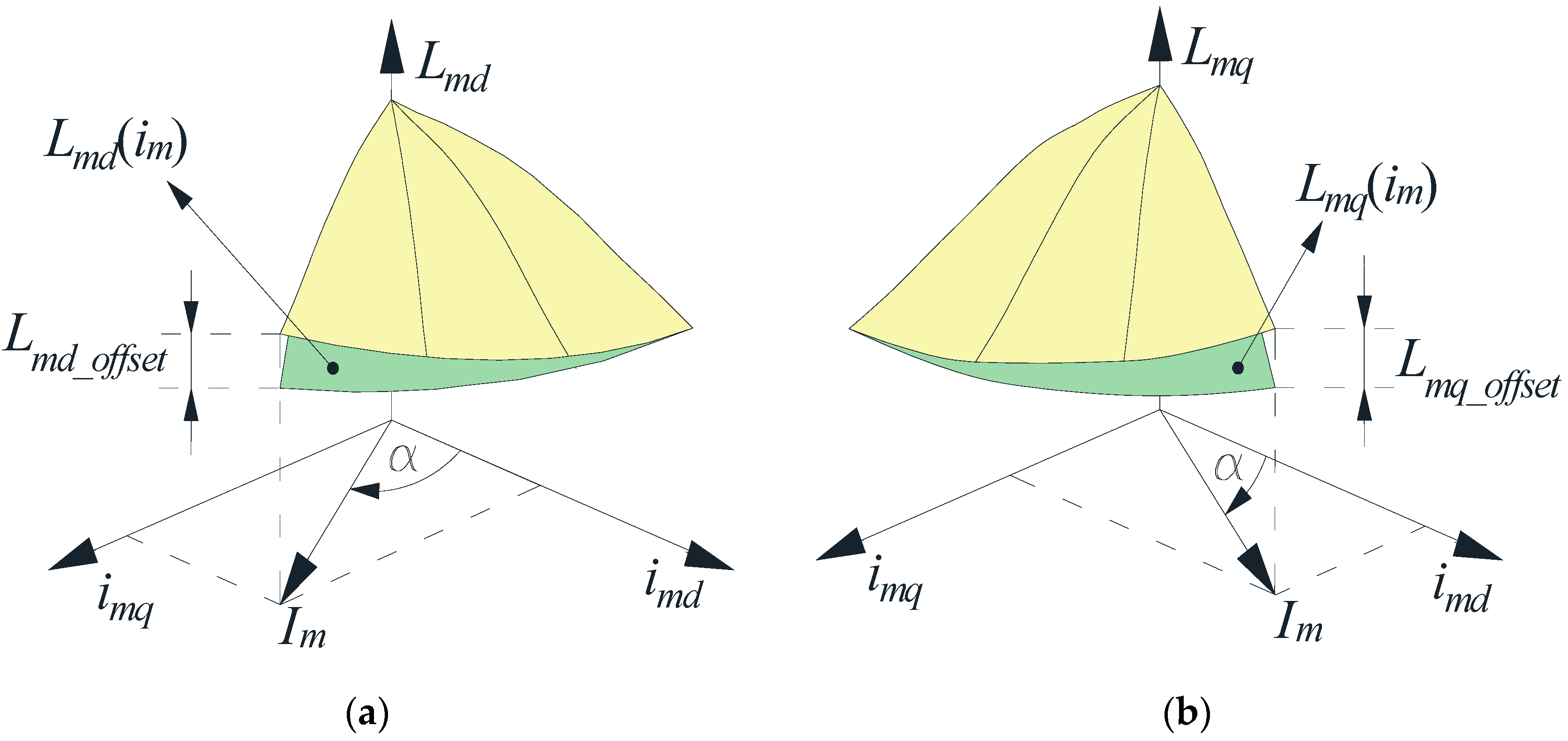
3. Analytical Methods for Determining the Flux Linkage Map

In this section, three analytical methods for determining the machine’s flux linkage map based on the measured magnetization curves in the d- and q-axis are briefly described.

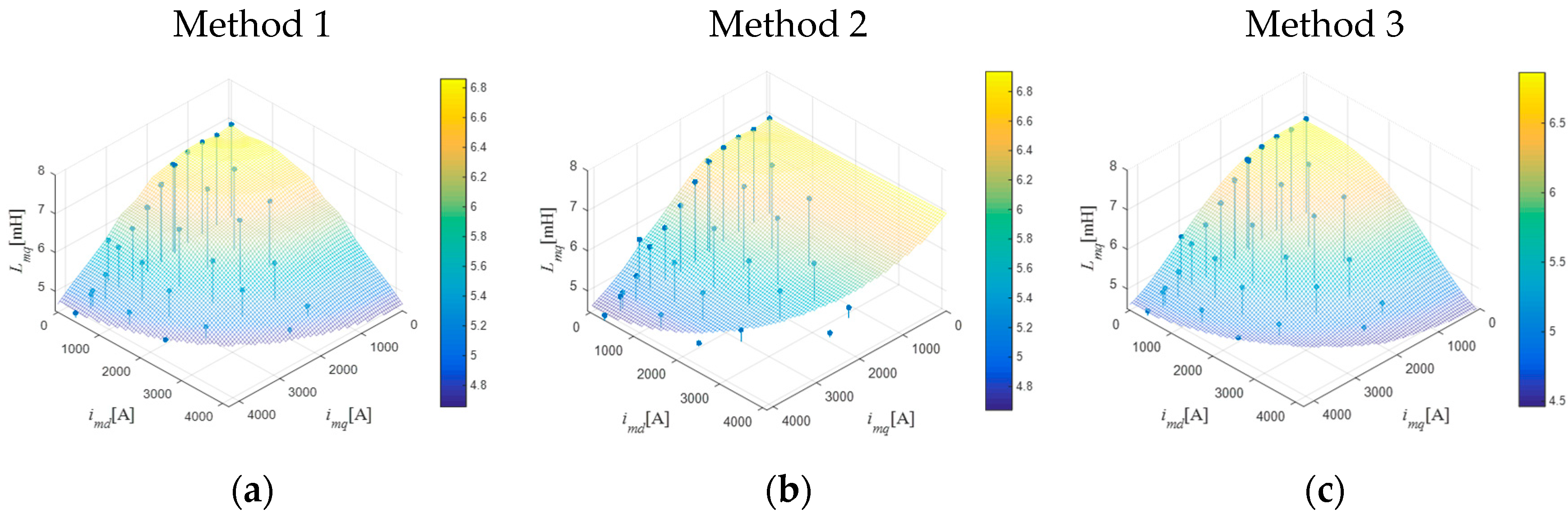
3.1. Method 1 (Levi)

The analytical method proposed by Levi in [31] allows the determination of the magnetizing inductance surfaces by knowing only the magnetization curve in the d-axis. In this method, a constant saliency factor defined as:

$$m=\sqrt{\frac{L_{mq\_uns}}{L_{md\_uns}}}=\sqrt{\frac{L_{mq}}{L_{md}}}=\mathrm{constant},$$

(6)

is assumed where L_{md_uns} and L_{mq_uns} are the unsaturated and L_md and L_mq are the saturated values of the magnetizing inductances. The d- and q-axis component of the magnetizing flux can be determined according to:

$$\begin{array}{l}{\psi }_{md}=L_{md}{i}_{md}=L_m\left(i_m\right)i_{md},\\ {\psi }_{mq}=L_{mq}{i}_{mq}=m^2{L}_m\left(i_m\right)i_{mq},\end{array}$$

(7)

where L_m and i_m are the magnetizing inductance and magnetizing current of an equivalent isotropic machine. The magnetizing inductance of the equivalent isotropic machine is determined based on the d-axis magnetization curve:

$$L_m(|i_m|)=L_{md}\left(i_{md},0\right)=L_{md}\left(i_{md}\right),$$

(8)

whereas the magnetizing current and the magnetizing flux are defined as:

$$\begin{array}{l}{i}_m=i_{md}+jm{i}_{mq},\\ {\psi }_m={\psi }_{md}+j{\psi }_{mq}/m.\end{array}$$

(9)

Figure 3 shows the space vectors of the magnetizing current and magnetizing flux (and their components) of an anisotropic and of an equivalent isotropic machine. One can notice that in an isotropic machine the space vectors of the magnetizing current and magnetizing flux are aligned.

3.2. Method 2 (Kaukonen)

In [7], Kaukonen proposed a method for the identification of the flux linkage map based on the so-called saliency-offset approach. Unlike the previously described method, this method requires knowledge of the magnetization curve in both the d- and q-axis. If the magnetization curves are defined as:

$$\begin{array}{l}{L}_{md}(i_{md})=L_{md}(i_{md},0),\\ L_{mq}(i_{mq})=L_{mq}(0,i_{mq}),\end{array}$$

(10)

the inductance surfaces can be determined by using the following expressions:

$$\begin{array}{l}{L}_{md}(i_{md},i_{mq})=L_{md}\left(\left|i_m\right|\right)+L_{md\_offset}\left(\angle \left(i_{md},i_{mq}\right),\left|i_m\right|\right),\\ L_{mq}(i_{md},i_{mq})=L_{mq}\left(\left|i_m\right|\right)+L_{mq\_offset}\left(\angle \left(i_{md},i_{mq}\right),\left|i_m\right|\right),\end{array}$$

(11)

where $i_m$ is the space vector of the magnetizing current, while $\angle \left(i_{md},i_{mq}\right)=\alpha$ and $\left|i_m\right|$ represent its modulus and angle, respectively. In expression (11) $L_{md}\left(\left|i_m\right|\right)$ and $L_{mq}\left(\left|i_m\right|\right)$ represent the inductance surfaces obtained by projecting the magnetization curves in the direction of the magnetizing current space vector, whereas $L_{md\_offset}$ and $L_{mq\_offset}$ represent the saliency-offset terms that are added to the obtained surfaces. According to [7], the saliency-offset terms $L_{md\_offset}$ and $L_{mq\_offset}$ are defined as:

$$\begin{array}{l}{L}_{md\_offset}=\sqrt{\frac{L_{mq\_uns}}{L_{md\_uns}}}{\left(\frac{\alpha }{\pi /2}\right)}^2\left(L_{md\_uns}-L_{md}\left(i_m\right)\right)\\ L_{mq\_offset}=\sqrt{\frac{L_{md\_uns}}{L_{mq\_uns}}}{\left(1-\frac{\alpha }{\pi /2}\right)}^2\left(L_{mq\_uns}-L_{mq}\left(i_m\right)\right)\end{array}$$

(12)

The principle of generating the magnetizing inductance surfaces used in [7] is shown in Figure 4, in accordance with expression (11) and (12). The author of [7] pointed out that the accuracy of the obtained inductance surfaces depends significantly on the accuracy of the saliency-offset. It should be also noted that Figure 4 shows only the principle of generating inductance surfaces, in other words, the saliency-offset in the q-axis does not necessarily take only positive values over the entire $i_{md},i_{mq}$ space.

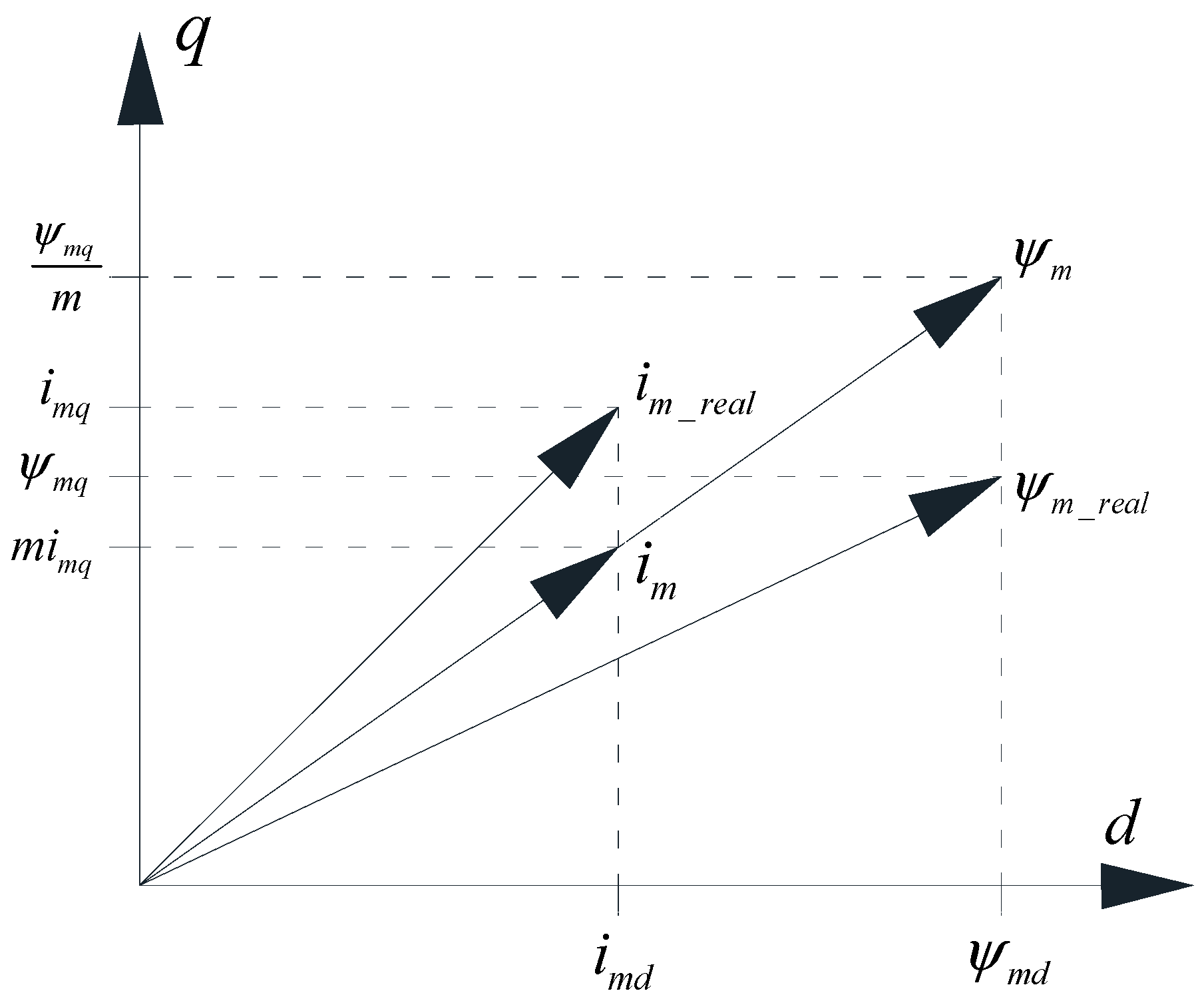
3.3. Method 3 (El-Serafi & Wu)

In [32] the flux linkage map, i.e., the inductance surfaces, were generated based on the magnetization curves of both the d- and q-axis. The method is explained in what follows, with all the relevant expressions, as well as illustrations, adopted from [32].

The method starts from the assumption that the magnetic field B at some point θ in the air gap can be described with:

$$B\left(\theta \right)=k_{1}F\left(\theta \right)\mu \left(\theta \right)S\left(\theta \right)$$

(13)

where θ is the angle of the considered point with respect to the d-axis, F(θ) is the magnetomotive force (MMF), μ(θ) is the equivalent unsaturated permeability along the air gap circumference, S(θ) is the MMF dependent saturation factor and k₁ is a constant that depends on the geometry of the machine. The change of the equivalent unsaturated permeability μ(θ) along the air gap can be seen from Figure 5, while saturation factor S(θ) is expressed as a n-th order polynomial:

$$S\left(\theta \right)=1-{\displaystyle \sum _{i=1}^n{a}_i}{{\displaystyle \left|F\left(\theta \right)\right|}}^i,$$

(14)

where a₁, a₂, …, a_n are machine dependent coefficients. The proposed model of the equivalent permeability is, as said, shown in Figure 5. The proposed model assumes that the equivalent permeability has a value of μ under the pole arc and zero value in the interpole region.

Based on Equations (13) and (14), the following expression can be derived:

$$B\left(\theta \right)=k_{1}F\left(\theta \right)\mu \left(\theta \right)\left(1-{\displaystyle \sum _{i=1}^n{a}_i}{{\displaystyle \left|F\left(\theta \right)\right|}}^i\right)$$

(15)

In this method, a Fourier series analysis was applied to Equation (15) in order to determine the fundamental components of the magnetizing flux density in the d- and q-axis. Integrating the obtained fundamental components over one pole pitch results in the following expressions for the fundamental components of the magnetizing flux in the d- and q-axis:

$$\begin{array}{l}{\psi }_{md}=\frac{2}{\pi }{\displaystyle \underset{-\tau /2}{\overset{\tau /2}{\int }}kF\left(\theta \right)\left(1-{\displaystyle \sum _{i=1}^n{a}_i}{{\displaystyle \left|F\left(\theta \right)\right|}}^i\right)\cos }\left(\theta \right)d\theta ,\\ {\psi }_{mq}=\frac{2}{\pi }{\displaystyle \underset{-\tau /2}{\overset{\tau /2}{\int }}kF\left(\theta \right)\left(1-{\displaystyle \sum _{i=1}^n{a}_i}{{\displaystyle \left|F\left(\theta \right)\right|}}^i\right)\sin }\left(\theta \right)d\theta ,\end{array}$$

(16)

where k is a machine dependent constant that can be treated as the equivalent unsaturated permeance of the machine [32]. The saturation factor coefficient a₁, a₂, …, a_n, as well as the pole arc width τ and the aforementioned equivalent permeance are not known in advance. In order to determine these unknown parameters, the no-load magnetization curves in the d- and q-axis are used. If the current flows only in the d- or q-axis, the following expression can be obtained:

$$\begin{array}{l}{\psi }_{md}=\frac{2k}{\pi }{\displaystyle \underset{-\tau /2}{\overset{\tau /2}{\int }}{I}_{d\_AT}\cos \left(\theta \right)\left(1-{\displaystyle \sum _{i=1}^n{a}_i}{{\displaystyle \left|F\left(\theta \right)\right|}}^i\right)\cos }\left(\theta \right)d\theta ,\\ {\psi }_{mq}=\frac{2k}{\pi }{\displaystyle \underset{-\tau /2}{\overset{\tau /2}{\int }}{I}_{q\_AT}\sin \left(\theta \right)\left(1-{\displaystyle \sum _{i=1}^n{a}_i}{{\displaystyle \left|F\left(\theta \right)\right|}}^i\right)\cos }\left(\theta \right)d\theta ,\end{array}$$

(17)

where $F_d\left(\theta \right)=I_{d\_AT}\cos \left(\theta \right)$ and $F_q\left(\theta \right)=I_{q\_AT}\sin \left(\theta \right)$ are the MMFs of the d- and q-axis, respectively. By calculating the integrals in Equation (16), the following expressions for the d- and q-axis magnetization curves are obtained:

$$\begin{array}{l}{\lambda }_{md}\left(I_{md\_AT}\right)=L_{md}\left(I_{md\_AT}\right)I_{md\_AT}\\ \hspace{1em}\hspace{1em}\hspace{1em}\hspace{1em}\hspace{1em} =\left(c_0+a_1·c_1·I_{md\_AT}+a_2·c_2·{\left(I_{md\_AT}\right)}^2+\dots +a_n·c_n·{\left(I_{md\_AT}\right)}^n\right)I_{md\_AT}\\ {\lambda }_{mq}\left(I_{mq\_AT}\right)=L_{mq}\left(I_{mq\_AT}\right)I_{mq\_AT}\\ \hspace{1em}\hspace{1em}\hspace{1em}\hspace{1em}\hspace{1em} =\left(d_0+a_1·d_1·I_{mq\_AT}+a_2·d_2·{\left(I_{mq\_AT}\right)}^2+\dots +a_n·d_n·{\left(I_{mq\_AT}\right)}^n\right)I_{mq\_AT},\end{array}$$

(18)

where the constants c₀, c₁, …, c_n and d₀, d₁, …, d_n are defined in Appendix A in case when S(θ) is approximated with a fourth order polynomial. If the machine is unsaturated, it follows from Equation (17) that the unsaturated magnetizing inductances are:

$$\begin{array}{l}{L}_{md\_uns}=c_0=\frac{k}{\pi }\left(\tau +\sin \left(\tau \right)\right)\\ L_{mq\_uns}=d_0=\frac{k}{\pi }\left(\tau -\sin \left(\tau \right)\right).\end{array}$$

(19)

If L_{md_uns} and L_{mq_uns} are known, the pole arc width and the equivalent permeance k can be calculated from Equation (18). Furthermore, from Equation (17) the following system of linear equations can be written:

$$\left[\begin{array}{c}{L}_{md,1}-c_0\\ L_{md,2}-c_0\\ ⋮\\ L_{md,L}-c_0\\ L_{mq,1}-d_0\\ L_{mq,2}-d_0\\ ⋮\\ L_{mq,M}-d_0\end{array}\right]=\left[\begin{array}{cccc}{c}_1\left(I_{d\_AT,1}\right)& c_2{\left(I_{d\_AT,1}\right)}^2& \cdots & c_n{\left(I_{d\_AT,1}\right)}^n\\ c_1\left(I_{d\_AT,2}\right)& c_2{\left(I_{d\_AT,2}\right)}^2& \cdots & c_n{\left(I_{d\_AT,2}\right)}^n\\ ⋮& ⋮& ⋮& ⋮\\ c_1\left(I_{d\_AT,L}\right)& c_2{\left(I_{d\_AT,L}\right)}^2& \cdots & c_n{\left(I_{d\_AT,L}\right)}^n\\ d_1\left(I_{q\_AT,1}\right)& d_2{\left(I_{q\_AT,1}\right)}^2& \cdots & d_n{\left(I_{q\_AT,1}\right)}^n\\ d_1\left(I_{q\_AT,2}\right)& d_2{\left(I_{q\_AT,2}\right)}^2& \cdots & d_n{\left(I_{q\_AT,2}\right)}^n\\ ⋮& ⋮& ⋮& ⋮\\ d_1\left(I_{q\_AT,M}\right)& d_1{\left(I_{q\_AT,M}\right)}^2& \cdots & d_n{\left(I_{q\_AT,M}\right)}^n\end{array}\right]\left[\begin{array}{c}{a}_1\\ a_2\\ ⋮\\ a_n\end{array}\right],$$

(20)

where (I_{d_AT,1}, L_md,1), …, (I_{d_AT,L}, L_md,L) and (I_{q_AT,1}, L_mq,1), …, (I_{q_AT,M}, L_mq,M) are the measured data points of the no-load magnetization curves in the d- and q-axis. Expression (19) can be written in a more compact form as:

$$b=A·x.$$

(21)

The unknown coefficients of the saturation factor can be determined by solving Equation (20) using the least square method:

$$x={\left[\begin{array}{cccc}{a}_1& a_2& \cdots & a_n\end{array}\right]}^T={\left(A^{T}A\right)}^{-1}{A}^{T}b.$$

(22)

If the machine is excited from both the d- and q-axis, it is possible to define the total MMF as:

$$\begin{array}{c}{F}_{total}\left(\theta \right)=F_d\left(\theta \right)+F_q\left(\theta \right)\\ \hspace{1em}\hspace{1em}\hspace{1em}\hspace{1em}\hspace{1em}\hspace{1em}\hspace{1em}\hspace{1em}\hspace{1em}\hspace{1em}\hspace{1em}\hspace{1em}\hspace{1em}\hspace{1em}\hspace{1em}\hspace{1em}\hspace{1em} =I_{total\_AT}\cos \left(\alpha \right)\cos \left(\theta \right)+I_{total\_AT}\sin \left(\alpha \right)\sin \left(\theta \right)\\ \hspace{1em}\hspace{1em}\hspace{1em}\hspace{1em}\hspace{1em}\hspace{1em}\hspace{1em}=I_{total\_AT}\left(\cos \left(\alpha -\theta \right)\right),\end{array}$$

(23)

where the modulus and angle of the total MMF are:

$$\begin{array}{l}{I}_{total\_AT}=\sqrt{{\left(I_{d\_AT}\right)}^2+{\left(I_{q\_AT}\right)}^2},\\ \alpha =\mathrm{atan}\left(\frac{I_{q\_AT}}{I_{d\_AT}}\right).\end{array}$$

(24)

Finally, by substituting in Equation (22) into Equation (15), the following expressions are obtained:

$$\begin{array}{l}{\psi }_{md}=\frac{2k}{\pi }{I}_{total\_AT}{\displaystyle \underset{-\tau /2}{\overset{\tau /2}{\int }}\left(1-{\displaystyle \sum _{i=1}^n{a}_i}{{\displaystyle \left|F_{total}\left(\theta \right)\right|}}^i\right)\left(\cos \left(\alpha -\theta \right)\right)\cos }\left(\theta \right)d\theta \\ {\psi }_{mq}=\frac{2k}{\pi }{I}_{total\_AT}{\displaystyle \underset{-\tau /2}{\overset{\tau /2}{\int }}\left(1-{\displaystyle \sum _{i=1}^n{a}_i}{{\displaystyle \left|F_{total}\left(\theta \right)\right|}}^i\right)\left(\cos \left(\alpha -\theta \right)\right)\sin }\left(\theta \right)d\theta \end{array}$$

(25)

based on which it is possible to calculate the d- and q-axis of the magnetizing flux and thus generate the magnetizing inductance surfaces, for an arbitrary MMF value.

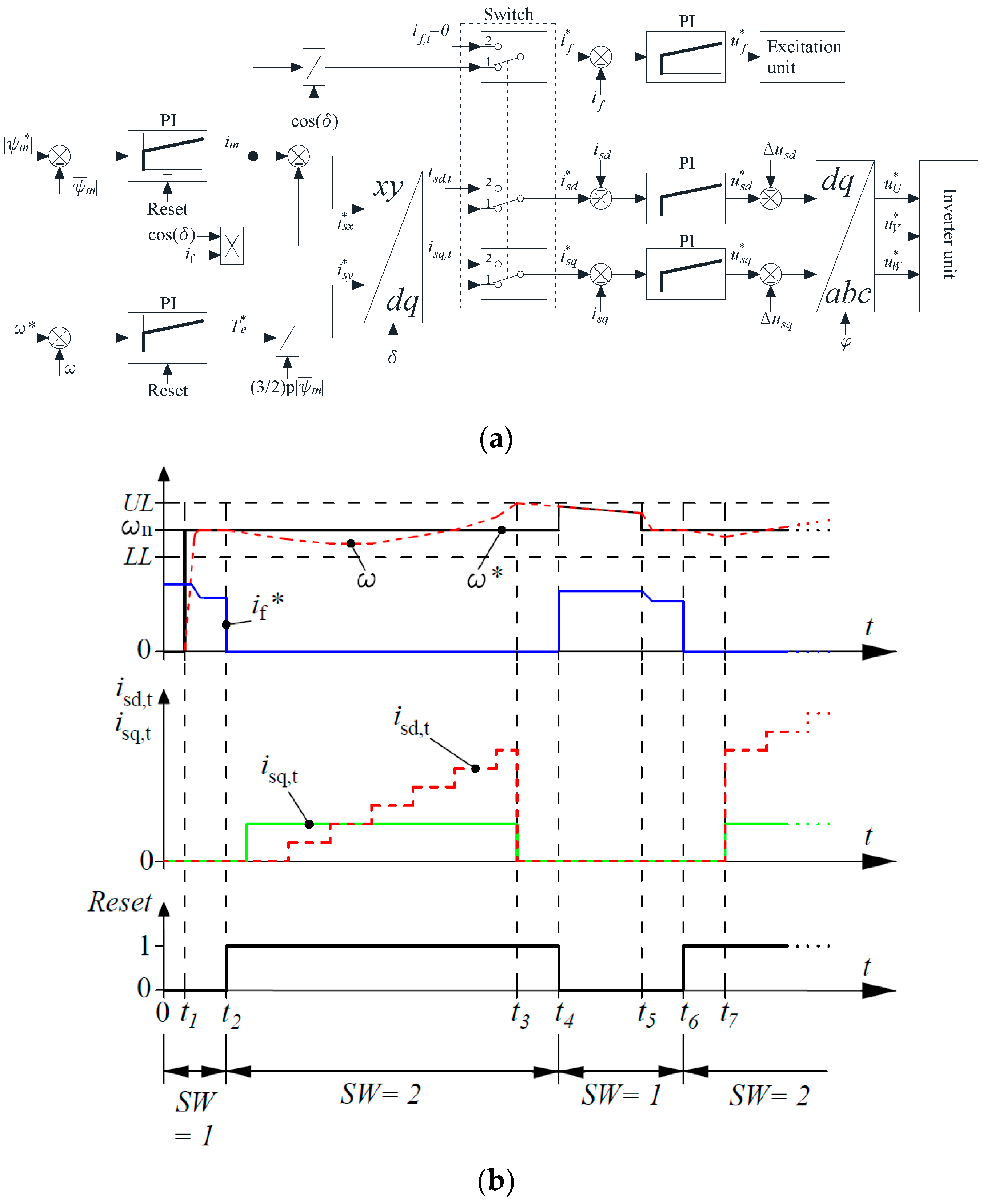
4. Description of the Proposed Experimental Method

Figure 6a shows the FOC structure used for the EESM drive which has been slightly modified in order to implement the experimental method. It should be noted that with this method the shaft of the machine can rotate freely during the flux linkage map identification process.

When the switch in Figure 6a is in position 1, the control structure acts like a conventional FOC structure used for controlling the speed of the machine. Moving the switch from position 1 to position 2 disables the outer speed and flux controllers, leaving only the inner current control loops, allowing the d- and q-axis stator current components to be injected into the machine according to a predefined pattern.

The signals of interest during the identification process are shown in Figure 6b. At the beginning, the switch is in position 1 and the machine accelerates to the nominal speed ω_n. During the acceleration phase, which lasts from t = 0 to t = t₂, the control structure acts as a conventional FOC structure, which is why the value of the field current is not zero. After the machine reaches its nominal speed at t = t₂, the switch is moved from position 1 to position 2, thus starting the injection of the stator current components which lasts until t = t₃. Thereby, the value of the field current is set to zero in order to minimize the developed torque of the machine and thus the change of the speed. The integration of PI controllers in the outer control loops is prevented by activating the Reset signal.

After the field current is brought to zero (immediately after t = t₂), the injection of the reference values for the d- and q-axis stator current components begins. Moreover, these references are injected according to a predefined pattern. An example of an injection pattern in which the q-axis current is kept constant and the d-axis current changes stepwise is shown in Figure 6b. For each operating point, the reference values of the stator current components are kept constant and the flux is calculated according to expression (5). However, the time interval of each operating point should be long enough for the stator currents, i.e., the magnetizing currents, to reach steady-state which results in a constant flux (please recall that expression (5) can be used only in case of a constant flux).

As shown in Figure 6b, a change in speed occurs during the injection of the stator current components due to friction and the presence of the machine’s reluctance torque. The speed of the machine is monitored throughout the current injection phase which is interrupted if the speed exceeds its defined upper limit (UL) or lower limit (LL). In Figure 6b, t₃ represents the time at which the speed exceeds its defined upper limit, after which the reference values of the d- and q-axis stator current components are set to zero. Once the values of these two currents become zero, the switch is at t = t₄ moved back to position 1 while the state of the Reset signal is changed from 1 to 0. From t = t₄ to t = t₆, the field current is once again raised and the acceleration of the machine begins. Once the speed of the machine reaches its nominal value, the switch is at t = t₆ moved again from position 1 to position 2, thus regulating the field current to zero. After that, the stator current components are again injected into the machine. The described process is repeated until the flux is determined in all operating points of interest.

The accuracy of the flux linkage map identification depends significantly on the precise knowledge of the fundamental harmonic of the stator voltages and currents. In order to avoid any error due to the estimation of the fundamental harmonic, the stator voltages and current were measured at the machine terminals and their fundamental harmonic determined using the Discrete Fourier Transform (DFT). Thereby, the voltages at the terminals were measured with medium-voltage probes, while the currents were measured using Rogowski current coils. The measuring probes were connected to two mutually synchronized oscilloscopes.

The utilization of the DFT was chosen because this type of transform is suitable for processing stationary signals, i.e., signals whose frequency content does not change over time [34]. However, although the change of the machine’s speed, which leads to nonstationary voltage and current signals, is inevitable for the proposed method, it can be ignored under assumption that the change in speed in a time interval corresponding to the window width of the DFT is negligibly small. Therefore, the window width of the DFT is chosen to be as small as possible, i.e., it is chosen to be equal to one electrical period. Since the speed of the machine, and therefore electrical frequency, changes during the identification process, the window width of the DFT must be exactly determined for each operating point in order to avoid any error in the determined fundamental component of the stator voltage and current. To determine the exact window width of the DFT a signal from an incremental encoder was used.

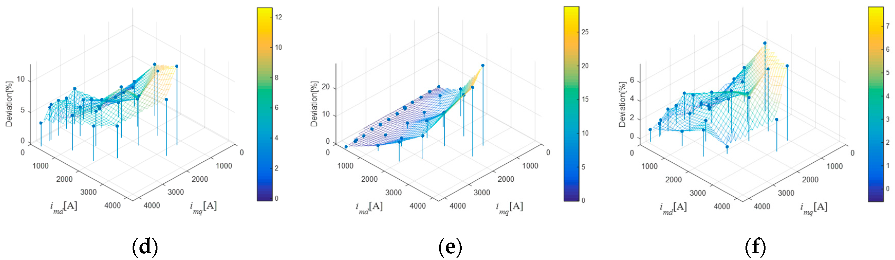
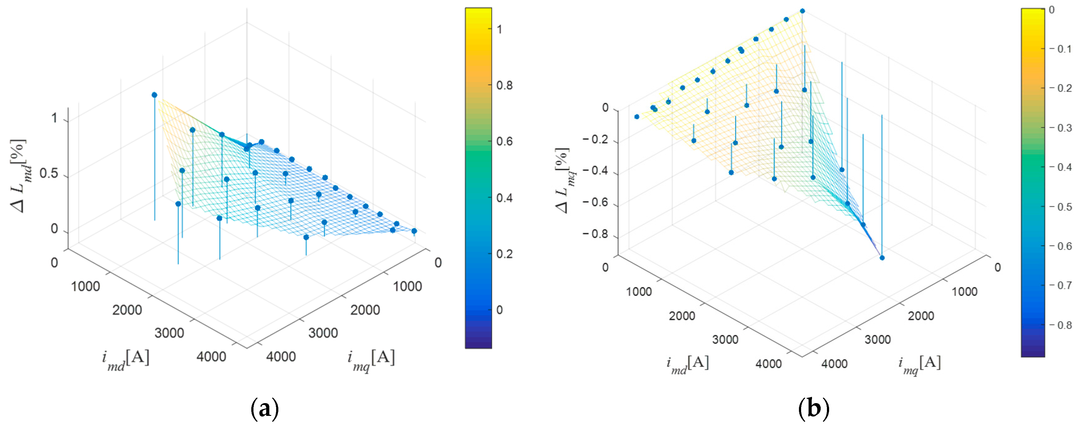
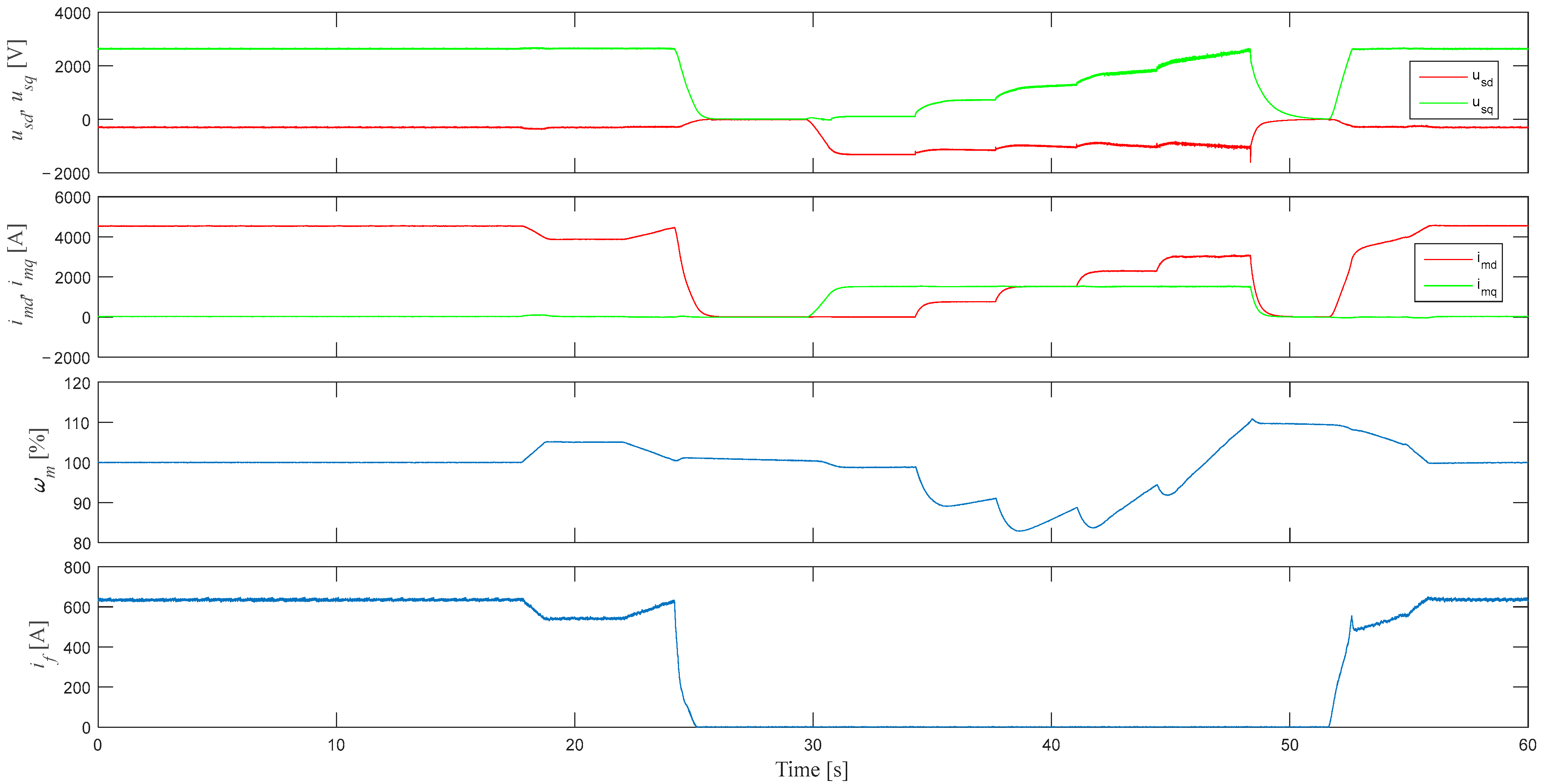
5. Experimental Verification of the Proposed Method

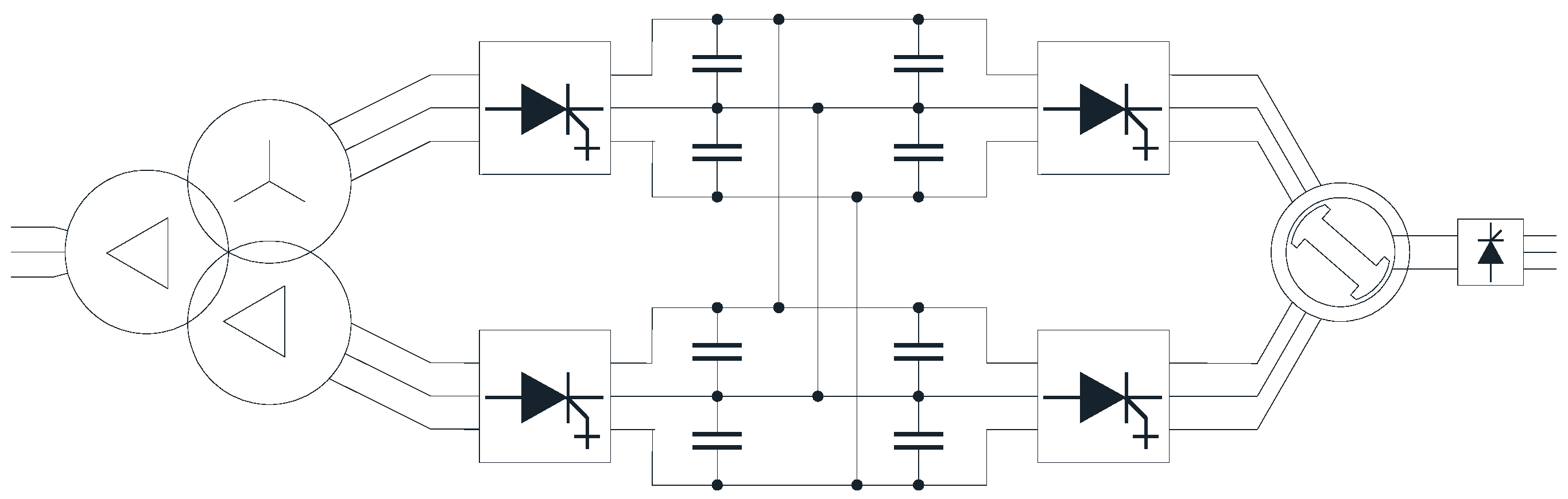
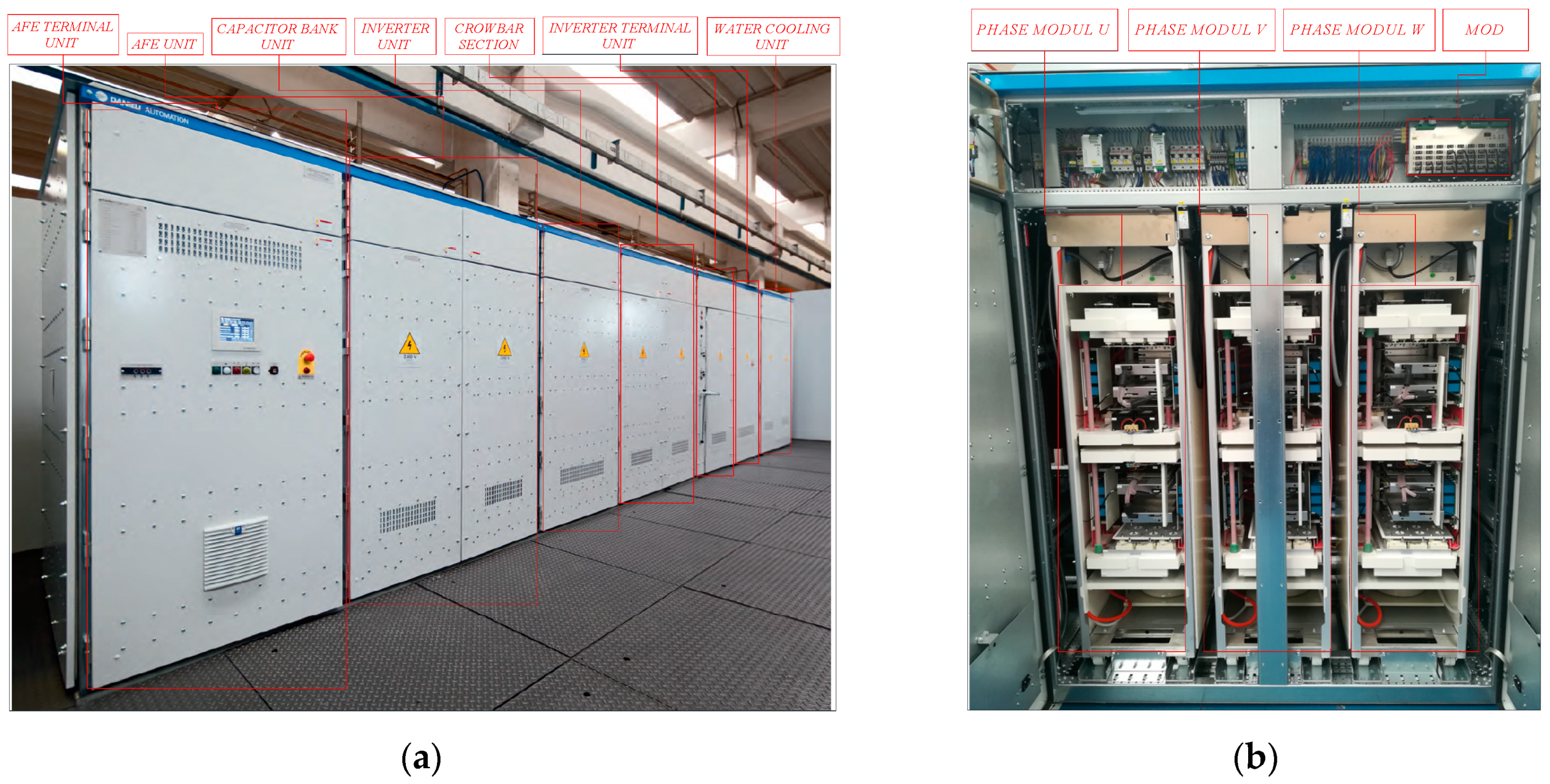
5.1. Experimental Setup

The experimental method proposed in this paper was used for the on-site identification of the flux linkage map of a medium-voltage EESM with double stator winding whose nominal data are given in

Table 1. Nominal data of the used EESM with double stator windings.

Parameter	Value
Nominal voltage	3050 V
Nominal current	2 × 1348 A
Nominal frequency	20 Hz
Nominal speed	200 rpm
Pole pair number	6
Nominal power	14 MW
Nominal field current	805 A

. On each of the two stator windings a medium-voltage three-level neutral point clamped (3L-NPC) inverter is connected, so that EESM is ultimately powered by two inverters. Both inverters are modulated using space vector modulation with a switching frequency of 300 Hz and have a common DC link (of 4800 V) which is powered using two active three-level rectifiers, each powered by a separate secondary winding of a step-down transformer. The modulation of these two rectifiers is based on a selective harmonic elimination algorithm. The power part of the medium-voltage drive in which the proposed experimental method was performed is shown in Figure 7.

Figure 8a shows the cabinet of the IGCT based medium-voltage drive, while Figure 8b shows an IGCT based 3L-NPC unit consisting of a central modulator unit (MOD) and phase modules where each IGCT module has an integrated gate unit.

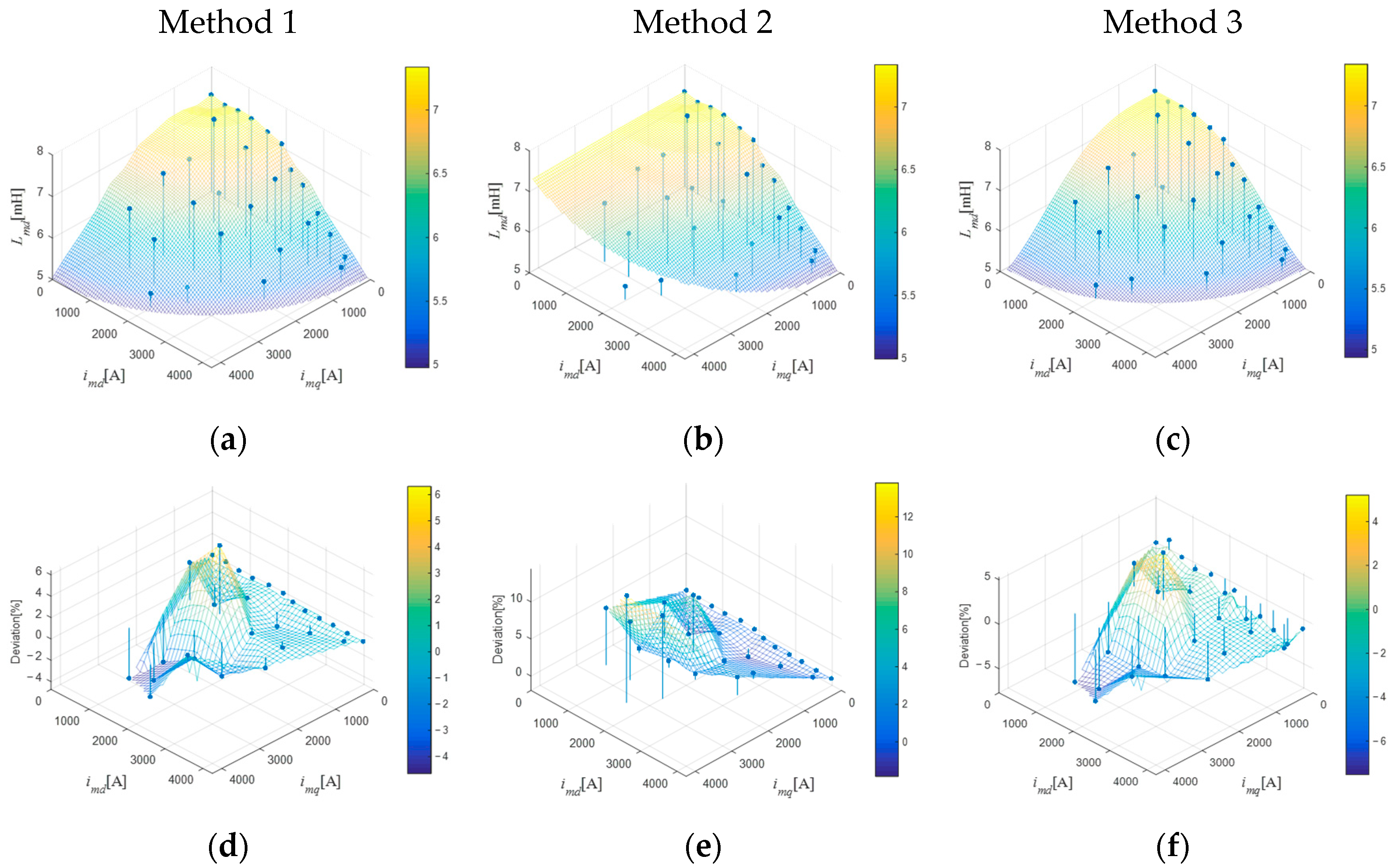
5.2. Experimental Results and Analysis

The proposed experimental method for flux linkage map identification has been implemented in a digital control system as described in Section 4. The proposed method was first used to determine the magnetization curve in the d- and q-axis. The d-axis magnetization curve obtained by using the proposed method and the one obtained by the standard open-circuit test are compared in Figure 9a. Unlike the open-circuit test which is based on injecting current into the field winding at a constant speed, in the method proposed, the speed is not constant and the current is injected only from the stator side. Good matching of the obtained d-axis magnetization curve with that taken from the machine’s test report implies the accuracy of the proposed method. In addition to the d-axis magnetization curve, the proposed method also allows the determination of the q-axis magnetization curve, which is shown in Figure 9b.

The comparison between the results obtained using the proposed method and the results obtained using analytical methods described in Section 3 in shown in Figure 10 and Figure 11, where the results obtained by the proposed method are represented with dots and the results obtained by analytical methods are represented with surfaces. Figure 10 refers to the d-axis magnetizing inductance, whereas Figure 11 refers to the q-axis magnetizing inductance. Thereby, the three Figure 11a–c are representing the comparison, while the three Figure 11d–f are representing the deviation between the results obtained by the proposed method and those obtained by using analytical methods. The comparison of the proposed method with the existing analytical methods is given in

Table A1. Comparison of the obtained L_md values.

			Method 1	Method 2	Method 3	Proposed Method
Nm.	$i_{md}\left[A\right]$	$i_{mq}\left[A\right]$	$L_{md}\left[mH\right]$	$L_{md}\left[mH\right]$	$L_{md}\left[mH\right]$	$L_{md}\left[mH\right]$
1.	0	0	7.33	7.33	7.33	7.33
2.	370	15	7.27	7.27	7.34	7.27
3.	741	31	7.33	7.33	7.33	7.33
4.	1110	42	7.32	7.32	7.23	7.32
5.	1499	11	7.19	7.19	7.17	7.19
6.	1874	7	7.08	7.08	6.97	7.08
7.	2250	137	6.71	6.71	6.70	6.71
8.	2606	168	6.53	6.53	6.37	6.53
9.	3001	175	6.05	6.05	5.97	6.05
10.	3352	179	5.73	5.73	5.61	5.73
11.	3751	192	5.39	5.39	5.23	5.39
12.	4174	198	4.98	4.98	4.96	4.98
13.	771	710	7.32	7.33	7.30	7.47
14.	1551	633	7.14	7.15	7.08	7.14
15.	2299	596	6.65	6.67	6.59	6.74
16.	3066	489	5.96	5.98	5.87	6.01
17.	3859	391	5.26	5.27	5.14	5.28
18.	845	1437	7.15	7.22	7.09	6.91
19.	1592	1394	6.87	6.94	6.80	6.46
20.	2363	1320	6.44	6.51	6.28	6.48
21.	3112	1270	5.74	5.82	5.6	5.77
22.	907	2193	6.68	7.02	6.59	6.98
23.	1675	2148	6.46	6.70	6.26	6.64
24.	2330	2081	5.98	6.23	5.85	6.19
25.	3297	1890	5.37	5.55	5.2	5.43
26.	753	2945	6.12	6.92	5.93	6.43
27.	1451	2988	5.84	6.53	5.64	6.06
28.	2360	3004	5.40	5.96	5.18	5.37
29.	1964	3597	5.15	6.08	5.00	5.31

and

Table A2. Comparison of the obtained L_mq values.

			Method 1	Method 2	Method 3	Proposed Method
Nm.	$i_{md}\left[A\right]$	$i_{mq}\left[A\right]$	$L_{mq}\left[mH\right]$	$L_{mq}\left[mH\right]$	$L_{mq}\left[mH\right]$	$L_{mq}\left[mH\right]$
1.	0	0	6.85	6.85	6.86	6.86
2.	9	373	6.79	6.81	6.86	6.81
3.	29	744	6.86	6.86	6.85	6.86
4.	47	1120	6.85	6.82	6.81	6.82
5.	63	1492	6.74	6.74	6.71	6.73
6.	112	1498	6.74	6.74	6.71	6.75
7.	146	1871	6.64	6.48	6.53	6.48
8.	151	1870	6.64	6.49	6.53	6.50
9.	186	2246	6.33	6.14	6.28	6.15
10.	197	2615	6.14	5.81	5.97	5.81
11.	194	2956	5.82	5.54	5.66	5.55
12.	293	3382	5.42	5.12	5.24	5.13
13.	315	3764	5.12	4.85	4.92	4.85
14.	328	4146	4.79	4.62	4.68	4.62
15.	771	710	6.85	6.84	6.82	6.58
16.	1551	633	6.68	6.76	6.61	6.16
17.	111	1496	6.74	6.74	6.71	6.73
18.	845	1438	6.69	6.65	6.63	6.53
19.	1592	1394	6.43	6.45	6.34	6.15
20.	2363	1320	6.02	6.27	5.81	5.45
21.	3112	1270	5.37	6.15	5.13	4.75
22.	187	2243	6.34	6.15	6.28	6.15
23.	907	2193	6.24	6.06	6.17	5.97
24.	1675	2148	6.04	5.93	5.84	5.58
25.	2330	2081	5.60	5.82	5.42	5.18
26.	3297	1890	5.02	5.77	4.76	4.6
27.	753	2945	5.73	5.5	5.58	5.47
28.	1451	2988	5.46	5.33	5.29	5.17
29.	2360	3004	5.05	5.20	4.83	4.80
30.	293	3691	5.18	4.90	4.97	4.90
31.	1134	3640	5.08	4.90	4.88	4.80
32.	1965	3597	4.82	4.88	4.69	4.56

, which can be found in Appendix B.

The deviation between the results obtained by using the proposed experimental method and the results obtained by using analytical methods has been calculated for each measured point. Thereby, the expression according to which the deviation of the results for the d-axis are calculated is:

$${\mathrm{Deviation}}_{d,k}[\%]=\frac{L_{md,analytical}\left(i_{md,k},i_{mq,k}\right)-L_{md,experimental}\left(i_{md,k},i_{mq,k}\right)}{L_{md,experimental}\left(i_{md,k},i_{mq,k}\right)}\times 100\%,$$

(26)

where (i_md,k, i_mq,k) represents the k-th measured data point. Analogously, the deviation of the results for the q-axis was calculated according to:

$${\mathrm{Deviation}}_{q,k}[\%]=\frac{L_{mq,analytical}\left(i_{md,k},i_{mq,k}\right)-L_{mq,experimental}\left(i_{md,k},i_{mq,k}\right)}{L_{mq,experimental}\left(i_{md,k},i_{mq,k}\right)}\times 100\%.$$

(27)

The rate showing how well an analytical method describes the experimentally obtained results is based on the L2 norm:

$$\begin{array}{l}{\left|{\mathrm{Deviation}}_d\right|}_2=\sqrt{{\mathrm{Deviation}}_{d,1}^2+{\mathrm{Deviation}}_{d,2}^2+\dots },\\ {\left|{\mathrm{Deviation}}_q\right|}_2=\sqrt{{\mathrm{Deviation}}_{q,1}^2+{\mathrm{Deviation}}_{q,2}^2+\dots }.\end{array}$$

(28)

The calculated values of the L2 norms are given in

Table 2. Calculated L2 norms for the deviations between the experimentally and analytically obtained results.

	Method 1	Method 2	Method 3
$L_{md}$	11.9	23.3	19.2
$L_{mq}$	31.1	46.8	17.4

for both magnetizing inductance and for all three analytical methods. It can be seen that the results obtained by Method 1 best match the results obtained by the proposed experimental method when it comes to determining the d-axis magnetizing inductance. On the other hand, when it comes to determining the q-axis magnetizing inductance, it can be seen that the results obtained by Method 3 better match the experimental obtained results than the other two analytical methods.

Furthermore, a potential problem related to the change of the input frequency has been also analyzed. It has been concluded that the change in electrical frequency can be neglected for all operating points. This analysis was performed by numerical calculation of the speed derivatives for all operating points. For example, the biggest impact on the accuracy of the proposed experimental method was recorded for the operating point at which the values of the magnetizing currents were i_md = 2312 A and i_mq = 2968 A, at 110% of the nominal speed. At this operating point, the time derivative of the electrical frequency was:

$$\frac{d{\mathrm{f}}_{el.}}{dt}=2.3\left[\frac{\mathrm{Hz}}{\mathrm{s}}\right]$$

(29)

At 110% of the nominal speed, the electrical frequency is 22 Hz, which means that one electrical period is T_el = 1/22 = 0.0455 s. Hence, the change of frequency in one interval of the DFT window is:

$$\Delta {\mathrm{f}}_{el.}=\frac{d{\mathrm{f}}_{el.}}{dt}\Delta t=2.3·0.0455=0.105 \mathrm{Hz},$$

(30)

which in percentages equals to:

$$\Delta {\mathrm{f}}_{el.}[\%]=\frac{0.105}{22}\times 100\%=0.48\%,$$

(31)

Since the proposed method was used for the identification of the flux linkage map of a high-power machine, considering the influence of the stator resistance change during the calculation of the flux was not necessary as it was assumed, because of the size of the machine, that the voltage drop on the stator resistance is negligible compared to the induced back EMF. However, in order to confirm this assumption, a percentage change in the inductance due to the increase in the stator resistance value was calculated based on the following expressions:

$$\begin{array}{l}\Delta L_{md}[\%]=\frac{L_{md,Rs}-L_{md,1.5\times Rs}}{L_{md,Rs}}\times 100\%,\\ \Delta L_{mq}[\%]=\frac{L_{mq,Rs}-L_{mq,1.5\times Rs}}{L_{mq,Rs}}\times 100\%.\end{array}$$

(32)

Figure 12 shows the percentage change in the value of the magnetizing inductances in case of a resistance increase of 50% with respect to its nominal value. As can be seen from Figure 12, almost all of the percentage changes are less than 1% (with 1.11% being the only change above 1%) which leads to the conclusion that even a significant change in resistance causes a negligible error in the obtained inductances.

The d- and q-axis components of the stator voltage and magnetizing current, as well as the speed and field current are shown in Figure 13 for the case when the reference value of the q-axis stator current component is i_sq,t = 40% and the reference value of the d-axis stator current component i_sd,t changes from 0 to 80% of the nominal current value in step of 20% (from t = 30 until t = 45 s).

Figure 14 shows the waveforms of the voltages and currents measured directly at the terminals of the machine for one electrical period in case of stator current component reference values of i_sq,t = 40% and i_sd,t = 80% of the nominal current. It should be emphasized that the waveform shown in Figure 14b represents the total current obtained as the sum of the currents of each winding of the machine.

6. Conclusions

This paper presents a novel experimental method for the identification of the flux linkage map of a medium-voltage EESM with double stator winding in case where it is not possible to use a complex laboratory-like experimental setup or perform FEM simulations without knowing the exact geometry, i.e., construction of the machine. The proposed method was implemented by modifying the existing FOC algorithm in the digital control system. In order to avoid problems due to the nonlinearities of the inverter, the stator voltage was measured using voltage probes after which its first harmonic was obtained by using Fourier analysis. The proposed method is suitable for synchronous machines with controllable excitation, i.e., electrically excited synchronous machines (EESMs), in which the reluctance torque does not lead to a significant change in the machine’s speed (in one electrical period) during the identification process. Therefore, it can be concluded that the proposed method is suitable for high-power EESMs that have a relatively high inertia.

Using the proposed method, the magnetization curves i the d- and q-axis were determined, and the accuracy of the proposed methods was verified by comparing the obtained magnetization curve in the d-axis with that obtained by the standard open-circuit test—increasing the field current at constant speed. It has been shown that the proposed experimental method can be also used to determine the magnetization curve in the q-axis, which cannot be done by the standard open-circuit test. Furthermore, based on the obtained magnetization curves, the flux linkage map of the EESM was generated, whereby the performed sensitivity analysis showed that the change in resistance value has a negligible impact on the obtained results, i.e., on the obtained flux linkage map. Acceptable accuracy confirmed by comparison with three different analytical methods, together with the fact that it does not require a complex experimental setup, makes the proposed method suitable for the identification of a machine’s flux linkage map in an industrial environment. Although the proposed method was applied to identify the flux-linkage map of a synchronous machine with a double stator winding, it can be applied to standard synchronous machines (with a single stator winding) as well.

References

1. Niemelä, M. Position Sensorless Electrically Excited Synchronous Motor Drive for Industrial Use Based on Direct Flux Linkage and Torque Control. Ph.D. Thesis, Lappeenranta University of Technology, Lappeenranta, Finland, 16 April 1999. [Google Scholar]
2. Boldea, I.; Nasar, S.A. Electric Drives, 3rd ed.; CRC Press, Taylor & Francis Group: Boca Raton, FL, USA, 2016. [Google Scholar]
3. Tao, L.; Sun, J.; Tian, Z.; Huang, M.; Zha, X.; Gong, J. Speed-Sensorless and Motor Parameters-Free Starting Method for Large-Capacity Synchronous Machines Based on Virtual Synchronous Generator Technology. IEEE Trans. Ind. Electron. 2020, 68, 6607–6618. [Google Scholar] [CrossRef]
4. Vas, P. Vector Control of AC Machines; Oxford University Press: New York, NY, USA, 1990. [Google Scholar]
5. Cikač, D.; Turk, N.; Bulić, N.; Barbanti, S. Flux Estimator for Salient Pole Synchronous Machines Driven by the Cycloconverter Based on Enhanced Current and Voltage Model of the Machine with Fuzzy Logic Transition. Machines 2021, 9, 279. [Google Scholar] [CrossRef]
6. Pyrhönen, J.; Hrabovcová, V.; Semken, R.S. Electrical Machine Drives Control, 1st ed.; John Wiley & Sons: Chichester, UK, 2016. [Google Scholar]
7. Kaukonen, J. Salient Pole Synchronous Machine Modelling in an Industrial Direct Torque Controlled Drive Application. Ph.D. Thesis, Lappeenranta University of Technology, Lappeenranta, Finland, 26 March 1999. [Google Scholar]
8. Han, Y.; Wu, X.; He, G.; Hu, Y.; Ni, K. Nonlinear Magnetic Field Vector Control with Dynamic-Variant Parameters for High-Power Electrically Excited Synchronous Motor. IEEE Trans. Power Electron. 2020, 35, 11053–11063. [Google Scholar] [CrossRef]
9. Cai, F.; Li, K.; Sun, X.; Wu, M. Air-Gap Flux Oriented Vector Control Based on Reduced-Order Flux Observer for EESM. Energies 2021, 14, 5874. [Google Scholar] [CrossRef]
10. Graus, J.; Hahn, I. Improved accuracy of sensorless position estimation by combining resistance- and inductance-based saliency tracking. In Proceedings of the IECON 2015—41st Annual Conference of the IEEE Industrial Electronics Society, Yokohama, Japan, 9–12 November 2015. [Google Scholar]
11. Li, H.; Huang, S.; Luo, D.; Gao, J.; Fan, P. Dynamic DC-link Voltage Adjustment for Electric Vehicles Considering the Cross Saturation Effects. Energies 2018, 11, 2046. [Google Scholar] [CrossRef] [Green Version]
12. Jeong, I.; Kim, J.; Kim, Y.; Nam, K. Extended MTPA with cross coupling inductances for electrically excited synchronous motors. In Proceedings of the IEEE Energy Conversion Congress and Exposition, Denver, CO, USA, 15–19 September 2013. [Google Scholar]
13. Tang, J.; Liu, Y. Design and Experimental Verification of a 48 V 20 kW Electrically Excited Synchronous Machine for Mild Hybrid Vehicles. In Proceedings of the 13th International Conference on Electrical Machines (ICEM), Alexandroupoli, Greece, 3–6 September 2018. [Google Scholar]
14. Kim, Y.; Nam, K. Copper-Loss-Minimizing Field Current Control Scheme for Wound Synchronous Machines. IEEE Trans. Power Electron. 2016, 32, 1335–1345. [Google Scholar] [CrossRef]
15. Jeong, I.; Gu, B.G.; Kim, J.; Nam, K.; Kim, Y. Inductance Estimation of Electrically Excited Synchronous Motor via Polynomial Approximations by Least Square Method. IEEE Trans. Ind. Appl. 2015, 51, 1526–1537. [Google Scholar] [CrossRef]
16. Koteich, M. Flux estimation algorithms for electric drives: A comparative study. In Proceedings of the 3rd International Conference on Renewable Energies for Developing Countries (REDEC), Zouk Mosbeh, Lebanon, 13–15 July 2016. [Google Scholar]
17. Sharma, T.; Bhattacharya, A.; Ahmed, H. Transient and steady-state study of a speed sensorless IPMSM drive with an advanced integrator-based stator flux estimator. IET Power Electron. 2021, 14, 1157–1172. [Google Scholar] [CrossRef]
18. Holtz, J.; Quan, J. Drift- and parameter-compensated flux estimator for persistent zero-stator-frequency operation of sensor-less-controlled induction motors. IEEE Trans. Ind. Appl. 2003, 39, 1052–1060. [Google Scholar] [CrossRef]
19. Vasic, V.; Vukosavic, S.N.; Levi, E. A stator resistance estimation scheme for speed sensorless rotor flux oriented induction motor drives. IEEE Trans. Energy Convers. 2003, 18, 476–483. [Google Scholar] [CrossRef] [Green Version]
20. Kim, H.-S.; Sul, S.-K.; Yoo, H.; Oh, J. Distortion-Minimizing Flux Observer for IPMSM Based on Frequency-Adaptive Observers. IEEE Trans. Power Electron. 2019, 35, 2077–2087. [Google Scholar] [CrossRef]
21. Boldea, I.; Agarlita, S.C. The active flux concept for motion-sensorless unified AC drives: A review. In Proceedings of the International Aegean Conference on Electrical Machines and Power Electronics and Electromotion (ACEMP), Istanbul, Turkey, 8–10 September 2011. [Google Scholar]
22. Wang, D.; Lu, K.; Rasmussen, P.O. Improved Closed-Loop Flux Observer Based Sensorless Control Against System Oscillation for Synchronous Reluctance Machine Drives. IEEE Trans. Power Electron. 2019, 34, 4593–4602. [Google Scholar] [CrossRef] [Green Version]
23. Jo, G.-J.; Choi, J.-W. Gopinath Model-Based Voltage Model Flux Observer Design for Field-Oriented Control of Induction Motor. IEEE Trans. Power Electron. 2018, 34, 4581–4592. [Google Scholar] [CrossRef]
24. Armando, E.G.; Bojoi, I.R.; Guglielmi, P.; Pellegrino, G.; Pastorelli, M.A. Experimental Identification of the Magnetic Model of Synchronous Machines. IEEE Trans. Ind. Appl. 2013, 49, 2116–2125. [Google Scholar] [CrossRef]
25. Rahman, K.M.; Hiti, S.S. Identification of machine parameters of a synchronous motor. In Proceedings of the 38th IAS Annual Meeting on Conference Record of the Industry Applications Conference, Salt Lake City, UT, USA, 12–16 October 2003. [Google Scholar]
26. Pellegrino, G.; Boazzo, B.B.; Jahns, T.M. Magnetic Model Self-Identification for PM Synchronous Machine Drives. IEEE Trans. Ind. Appl. 2015, 51, 2246–2254. [Google Scholar] [CrossRef] [Green Version]
27. Liu, K.; Feng, J.; Guo, S.; Xiao, L.; Zhu, Z.-Q. Identification of Flux Linkage Map of Permanent Magnet Synchronous Machines Under Uncertain Circuit Resistance and Inverter Nonlinearity. IEEE Trans. Ind. Inform. 2017, 14, 556–568. [Google Scholar] [CrossRef]
28. Odhano, S.A.; Bojoi, R.; Rosu, S.G.; Tenconi, A. Identification of the magnetic model of permanent magnet synchronous machines using DC-biased low frequency AC signal injection. IEEE Trans. Ind. Appl. 2015, 51, 3208–3215. [Google Scholar] [CrossRef]
29. Stumberger, B.; Dolinar, D.; Hamler, A.; Trlep, M. Evaluation of saturation and cross-magnetization effects in interior permanent-magnet synchronous motor. IEEE Trans. Ind. Appl. 2003, 39, 1264–1271. [Google Scholar] [CrossRef]
30. El-Serafi, A.M.; Kar, N.C. Methods for determining the intermediate-axis saturation Characteristics of salient-pole synchro-nous Machines from the measured D-axis Characteristics. IEEE Trans. Energy Convers. 2005, 20, 88–97. [Google Scholar] [CrossRef]
31. Levi, E. Saturation modelling in d-q axis models of salient pole synchronous machines. IEEE Trans. Energy Convers. 1999, 14, 44–50. [Google Scholar] [CrossRef]
32. El-Serafi, A.M.; Wu, J. A new method for determining the saturation curves in the intermediate axes of salient-pole synchro-nous machines. Electr. Mach. Power Syst. 1993, 21, 199–216. [Google Scholar] [CrossRef]
33. Burzanowska, H.; Sario, P.; Stulz, C.A.; Joerg, P. Redundant Drive with Direct Torque Control (DTC) and dual-star synchro-nous machine, simulations and verification. In Proceedings of the European Conference on Power Electronics and Applications, Aalborg, Denmark, 2–5 September 2007. [Google Scholar]
34. Boashash, B. Time-Frequency Signal Analysis and Processing: A Comprehensive Reference, 2nd ed.; Academic Press: Cambridge, MA, USA, 2015. [Google Scholar]
Figure 1. Ref. [33] Equivalent circuits for the d- and q-axis of an EESM with double stator winding: (a) d-axis equivalent circuit; (b) q-axis equivalent circuit. The parameters of the equivalent circuits are as follows: R s is stator resistance, R D and R Q are the d- and q-axis damper winding resistances,   R f is the field resistance, L l s 1 and L l s 2 are the stator leakage inductances, L k d is the Canay inductance, L l s 1 _ 2 is the mutual leakage inductance between stator windings, L m d and L m q are the d- and q-axis magnetizing inductances, L l s D and L l s Q are the d- and q-axis damper winding leakage inductances, L l f is the field winding leakage inductance, u s d and u s q   are the d- and q-axis stator voltage components, i s d and i s q   are the d- and q-axis stator current components, ψ s d and ψ s q are the d- and q-axis stator flux components, and ω is the electrical speed.
Machines 10 00187 g001
Figure 2. Equivalent circuits for the d- and q-axis of the considered EESM with double star-connected stator winding: (a) d-axis equivalent circuit; (b) q-axis equivalent circuit.
Machines 10 00187 g002
Figure 3. Space vectors of the magnetizing current and magnetizing flux (and their components) of an anisotropic and of an equivalent isotropic machine.
Machines 10 00187 g003
Figure 4. The principle of generating magnetizing inductance surfaces as proposed in [6]: (a) d-axis magnetizing inductance surface; (b) q-axis magnetizing inductance surface.
Machines 10 00187 g004
Figure 5. Equivalent unsaturated permeability along the air-gap circumference (according to [32]).
Machines 10 00187 g005
Figure 6. (a) FOC structure of the EESM drive modified in order to implement the proposed experimental method (b) signals of interest during the flux linkage map identification process. (Reference signals are denoted with the asterisk sign).
Machines 10 00187 g006
Figure 7. Power part configuration of the MV drive unit.
Machines 10 00187 g007
Figure 8. (a) MV drive cabinet layout; (b) IGCT based 3L-NPC unit.
Machines 10 00187 g008
Figure 9. (a) comparison of obtained d-axis magnetization curve with that from a test report; (b) obtained q-axis magnetization curve.
Machines 10 00187 g009
Figure 10. Comparison between the obtained experimental and analytical results with corresponding deviations for the d-axis magnetizing inductance: (a,d) Method 1 (Levi); (b,e) Method 2 (Kaukonen); (c,f) Method 3 (El-Serafi & Wu).
Machines 10 00187 g010
Figure 11. Comparison between the obtained experimental and analytical results with corresponding deviations for the q-axis magnetizing inductance: (a,d) Method 1 (Levi); (b,e) Method 2 (Kaukonen); (c,f) Method 3 (El-Serafi & Wu).
Machines 10 00187 g011aMachines 10 00187 g011b
Figure 12. Percentage change of the obtained magnetizing inductances due to a 50% increase in stator resistance: (a) d-axis magnetizing inductance; (b) q-axis magnetizing inductance.
Machines 10 00187 g012
Figure 13. Waveforms of the considered machine during experimental verification of the method.
Machines 10 00187 g013
Figure 14. Waveforms of the voltages and currents measured at the machine terminals and their fundamental harmonics: (a) phase voltages, (b) total phase currents.
Machines 10 00187 g014