An Improved Deadbeat Current Controller of PMSM Based on Bilinear Discretization

Abstract

Based on the bilinear discretization mathematical model of permanent magnet synchronous motor (PMSM), an improved incremental deadbeat current prediction control algorithm is proposed. Aiming at the system instability caused by the forward Euler discretization method, this paper combines the deadbeat current prediction control and the improved bilinear discretization method to improve the system stability. Further, the proposed controller considers the two-beat delay of a digital system to make the mathematical model more accurate. Moreover, the proposed bilinear discretization predictive current controller is not affected by the permanent magnet flux of the motor. Then, the system stability conditions of the proposed controller are analyzed. The simulation and experimental results verify the feasibility and effectiveness of the proposed method.

1. Introduction

Control moment gyroscopes (CMGs) are important devices for attitude maneuverability of remote sensing satellites. The speed control performance of the CMG frame control system directly determines its attitude control performance. Therefore, a high-precision, high-bandwidth speed control is an important goal of the CMG frame control system. Permanent maget synchronous motors (PMSMs) have the characteristics of high-power density, good speed regulation performance, and rapid electrical torque response [1,2]. So, the PMSM is very suitable for the CMG frame system [3].

Since the dynamic current response is responsible for dynamic torque performance, a fast current-loop is the key factor in achieving a high steady-state precision and a fast dynamic torque response. In the current control for an inverter-fed PMSM drive, there are some main types of control schemes: the hysteresis control [4,5], direct torque control [6], sliding mode control [7,8], synchronous frame proportional integral (PI) control [9,10,11], fuzzy controller [12], and predictive current control [13,14,15]. The predictive controllers offer a fast response which is of great importance for CMG, so the predictive controller is used in this paper.

Predictive control techniques can be divided into two categories: finite control set model predictive control (FCS-MPC) [16] and deadbeat control [17]. The deadbeat structure is often used for current prediction where this method is called deadbeat prediction [18]. This method is based on the discrete motor model to predict voltage references [19]. The deadbeat current prediction control can accurately calculate the voltage vector of the next cycle according to the current command and the collected current and position information, so that the motor current can accurately follow the command current value. However, there are some problems in this method. The first problem is that the deadbeat current prediction control algorithm is sensitive to the mismatch of motor model parameters [20]. In the actual system, the motor parameters change with the operating state. The sensor has measurement error and acquisition delay, so the algorithm should be improved appropriately to accurately predict the current control.

The second problem is that the control delay of the digital control system, including the current sampling delay, duty ratio refreshing delay, and other factors, will greatly deteriorate the system’s control performance [21,22,23]. When the current predictive control algorithm of the PMSM is used in a digital platform, the delay is two sampling periods from the starting time of the current control to the sensing time of the resultant phase currents [13].

The other problem is that when implementing the traditional deadbeat control scheme, the traditional forward Euler method is used to discretize the PMSM mathematical model in the continuous domain. Although this method can simplify the discretization process, when the sampling time is large, it is difficult to balance the simplicity of the algorithm and the system stability. At the same time, if the MPC system needs to obtain high performance, the control sampling time should not be too long, and the calculation of the MPC controller should not be too complicated, otherwise the action delay will be generated. If the controller is not designed with these issues in mind, the resulting delay can deteriorate the system performance [24].

Therefore, aiming at the above problems, an improved incremental prediction model is established based on an improved bilinear discretization to further improve the system stability. The timing sequence of the current control in the digital control system with a two-sampling period delay is studied and the relationship between the currents at two-sampling period later and the reference current is obtained. By using the relationship, the implicit solution of the traditional bilinear discrete method can be changed to explicit solution. Moreover, by subtracting the discrete equations of adjacent cycles, the sensitive parameters such as the rotor flux of the motor can be eliminated. This paper analyzes the stability of the algorithm and derives the stability conditions of the algorithm. Simulation and experimental results verify the feasibility and effectiveness of the proposed method.

The remaining parts of this paper are organized as follows. Section 2 shows the discretization mathematical model of the PMSM. The deadbeat current predictive control algorithm of the PMSM in a digital platform is designed in Section 3. In Section 4, a bilinear discretization predictive current controller is developed and the stability of the control method is studied. In Section 5, simulations and experiments are carried out to show the performance of the proposed controller. Finally, the research conclusion is given in Section 6.

2. Discretization Mathematical Model of PMSM

2.1. Dynamic Equations of Stator Currents in PMSM

Assume that the employed PMSM has negligible cross-coupling magnetic saturation, structural asymmetry, iron losses, magnet eddy current loss, and harmonics in the descriptive functions of windings. In addition, rotor anisotropy and hysteresis are also ignored. The magnetic potential of each phase of the rotor is sinusoidally distributed in space. The dynamic equations of the stator currents of the PMSM in d-q coordinates can be given as follows [25]:

$$\frac{\mathrm{d}}{\mathrm{d}t}{i}_d=\frac{1}{L_d}\left(u_d-R{i}_d+\omega L_q{i}_q\right)$$

(1)

$$\frac{\mathrm{d}}{\mathrm{d}t}{i}_q=\frac{1}{L_q}\left(u_q-R{i}_q-\omega L_d{i}_d-\omega {\Psi }_f\right)$$

(2)

where ω is the electrical angular velocity of synchronously rotating d-q coordinates, u_d and u_q are the applied voltages in d-q coordinates, i_d and i_q are the current components in d-q coordinates, L_d and L_q are the equivalent inductances in d-q coordinates and L_d = L_q = L_s, R is the stator resistance per phase, and ψ_f is the flux linkage due to the permanent magnets. The rotor speed ω and magnetic flux ψ_f are considered constant during the sampling period.

2.2. Conventional Discretization Method

If the sampling period of the system is small enough, the rotor speed can be considered constant in a sampling period. The PMSM can be modeled in a discrete form using the first-order Taylor expansion:

$$X_{\left(k+1\right)}=A_{\left(k\right)}{X}_{\left(k\right)}+B{u}_{\left(k\right)}+d_{\left(k\right)}$$

(3)

where

$$X_{\left(k\right)}=\left[\begin{array}{l}{i}_{d\left(k\right)}\\ i_{q\left(k\right)}\end{array}\right], B=\left[\begin{array}{cc}\frac{T_s}{L_s}& 0\\ 0& \frac{T_s}{L_s}\end{array}\right], d_{\left(k\right)}=\left[\begin{array}{l}0\\ \frac{-T_s{\psi }_f{\omega }_{\left(k\right)}}{L_s}\end{array}\right], u_{\left(k\right)}=\left[\begin{array}{l}{u}_{d\left(k\right)}\\ u_{q\left(k\right)}\end{array}\right], A_{\left(k\right)}=\left[\begin{array}{cc}1-\frac{T_{s}R}{L_s}& T_s{\omega }_{\left(k\right)}\\ -T_s{\omega }_{\left(k\right)}& 1-\frac{T_{s}R}{L_s}\end{array}\right].$$

i_d(k), i_q(k), u_d(k) and u_q(k) are the d-q coordinates stator current and voltage at the kth sampling time, respectively. ω_(k) is the rotor electrical angular speed at the kth sampling time. T_S is sampling time.

In conventional predictive current control, optimal voltages should regulate currents to track their reference in one single sampling period when the sampling delay of the digital system and the effect of voltage output delay are not considered. From Equation (3), the optimal voltages are obtained as follows (when B is invertible):

$$u_{\left(k\right)}=B^{-1}\left(X_{\left(k+1\right)}^{ref}-A_{\left(k\right)}{X}_{\left(k\right)}-d_{\left(k\right)}\right)$$

(4)

where $X_{\left(k+1\right)}^{ref}={\left[i_{d\left(k+1\right)}^{ref}, i_{q\left(k+1\right)}^{ref}\right]}^{\mathrm{T}}$ is the reference value of X_(k+1), $i_{d\left(k+1\right)}^{ref}$ and $i_{q\left(k+1\right)}^{ref}$ are the reference current values at the (k + 1)th sampling time.

In the d-q coordinates, the Equation (4) is equivalent to

$$u_{d\left(k\right)}=R{i}_{d\left(k\right)}+\frac{L_s}{T_s}\left(i_{d\left(k+1\right)}^{ref}-i_{d\left(k\right)}\right)-{\omega }_k{L}_s{i}_{q\left(k\right)}$$

(5)

$$u_{q\left(k\right)}=R{i}_{q\left(k\right)}+\frac{L_s}{T_s}\left(i_{q\left(k+1\right)}^{ref}-i_{q\left(k\right)}\right)+{\omega }_k{L}_s{i}_{d\left(k\right)}+{\omega }_k{\psi }_f$$

(6)

The conventional predictive current controller is a kind of high gain proportional controller if the rotor speed and the back EMF terms are known and compensated properly.

2.3. Comparison of Discretization Method

From an intuitive point of view, if the sampling time is not sufficiently small with respect to the dynamics (frequency), the Tustin method (bilinear transformation) is more accurate than the Euler method since this approximation loses less area under the curve. The comparison of the trapezoidal integration and the Euler-based one is discussed below.

The forward Euler’s discretization formula is:

$$D_{\left(z\right)}=D_{\left(z\right)}{|}_{s=\frac{z-1}{T_s}}$$

(7)

The discretization formula of the bilinear transformation method is:

$$D_{\left(z\right)}=D_{\left(z\right)}{|}_{s=\frac{2z-1}{T_s\mathrm{z}-1}}$$

(8)

where T_s is the sampling period.

The mapping relationship between the s-plane and the z-plane of the two different discretization methods is as follows (letting s = δ + jω).

• Forward Euler Discretization formula

From Equation (7), we have

$$z=1+T_{s}s=\left(1+\delta T_s\right)+\mathrm{j}\omega T_s$$

(9)

$${\left|z\right|}^2={\left(1+\delta T_s\right)}^2+{\left(\omega T_s\right)}^2$$

(10)

Let |z| = 1 (unit circle), and then it corresponds to a circle on the s-plane.

$$\frac{1}{T_s^2}={\left(\frac{1}{T_s}+\delta \right)}^2+{\omega }^2$$

(11)

This indicates that only when all the poles of D_(s) are located in a circle at the left half-plane with the point (−1/T_s, 0) as the center and 1/T_s as the radius, are the poles of D_(z) after discretization at the z-plane located in the unit circle. This means that only part of the area on the s-plane can be mapped into the z-plane unit circle. That is, there exist cases in which D_(s) is stable, but D_(z) is not stable. Therefore, it is necessary to reduce the sampling period as it can improve the stability of D_(z).

• Bilinear transformation method.

It can be obtained from Equation (8):

$$z=\frac{1+\frac{T_s}{2}s}{1-\frac{T_s}{2}s}=\frac{\left(1+\frac{T_s}{2}\delta \right)+\mathrm{j}\frac{\omega T_s}{2}}{\left(1-\frac{T_s}{2}\delta \right)-\mathrm{j}\frac{\omega T_s}{2}}$$

(12)

Then, we have

$${\left|z\right|}^2=\frac{{\left(1+\frac{T_s}{2}\delta \right)}^2+{\left(\frac{\omega T_s}{2}\right)}^2}{{\left(1-\frac{T_s}{2}\delta \right)}^2+{\left(\frac{\omega T_s}{2}\right)}^2}$$

(13)

It can be known from Equation (13) that δ = 0 (on the s-plane imaginary axis) is mapped to |z| = 1 (on the z-plane unit circle); δ < 0 (left half s-plane) is mapped to |z| < 1 (within z-plane unit circle); and δ > 0 (right half s-plane) is mapped to |z| > 1 (outside the z-plane unit circle). From the above analysis, the bilinear transformation maps the entire left half s-plane to the z-plane unit circle. This mapping relationship indicates that if D_(s) is stable, the discrete D_(z) must also be stable. Compared with the forward Euler discretization method, the system stability after discretization using the bilinear variation method is no longer affected by the sampling frequency.

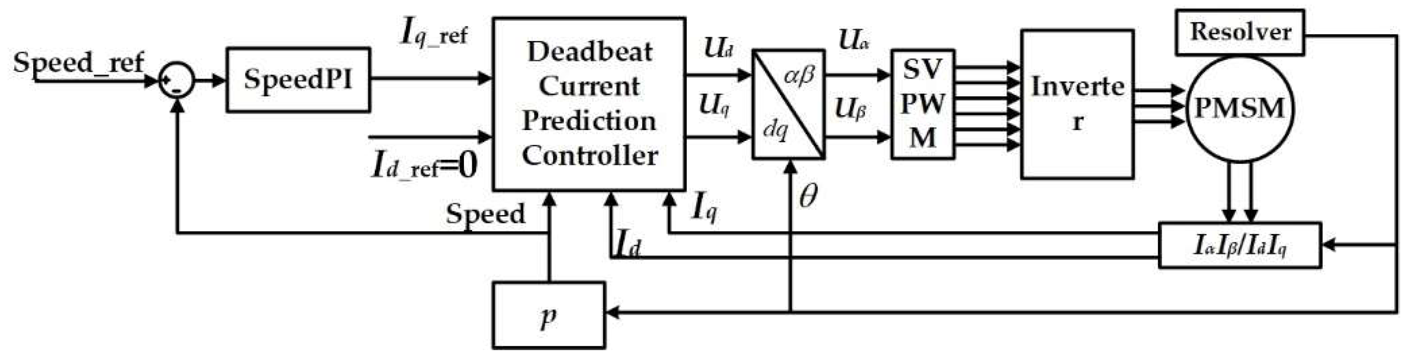
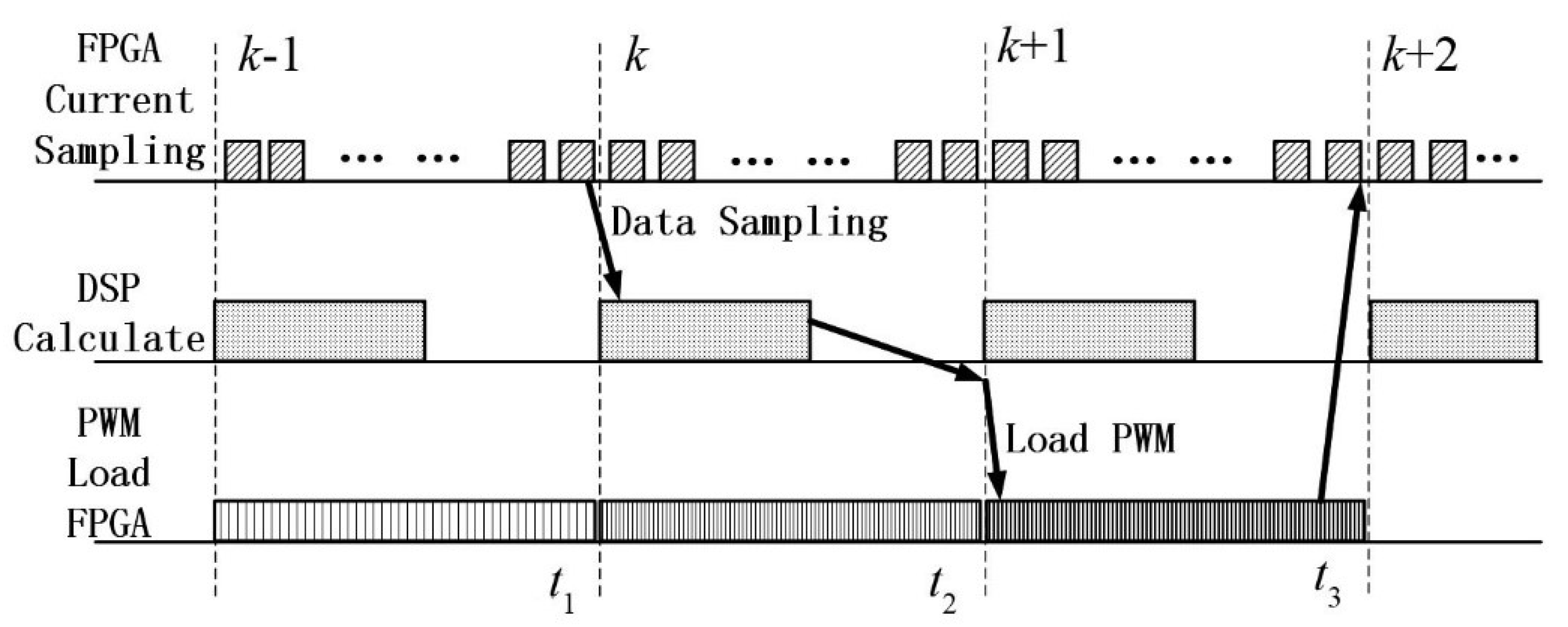
3. Deadbeat Current Predictive Control Algorithm of PMSM in the Digital Platform

The structure of the current prediction control algorithm proposed in this paper is shown in Figure 1. Combining predictive control with SVPWM, the deadbeat control idea is applied to predictive control to achieve a fast tracking of the reference current. In Figure 1, the output of the speed loop controller is used as the reference input of the deadbeat controller. The previous current sampling value is used to calculate the given voltage required by the SVPWM module. The deadbeat does not traverse the value function of the calculated vector, which is the major difference between deadbeat predictive control and conventional model predictive control. The deadbeat uses the given current value directly to predict the required voltage of the system. Then, the system generates a response switch signal through the SVPWM module. The system results in good performance with a fast dynamic response and lower current ripple.

Figure 2 shows the timing sequence of the current control in the digital control system. The operation interrupt signals are generated at time t_n (n = 1, 2…). The system comprises two parts: the main calculation processor is a digital signal processor (DSP), and the acquisition of signals and the generation of switching signals are performed by the FPGA. The k-th interrupt signal is generated at time t₁, as shown in Figure 2. Before the interrupt signal k, FPGA enables the AD converter to sample the current values, reading the rotor position from the resolver. At time t₁, FPGA sends the data required for DSP to calculate the output voltages. During the period from t₁ to t₂, the current controller needs to obtain the reference value of the PWM generator and upload the value using the internal interrupt. FPGA needs to apply the signals to the switches at time t₂. During the period from t₂ to t₃, the phase voltages calculated in the previous period are applied to the motor through the inverter. The current controller senses the current values at t₃, which is generated by the voltages calculated at t₁.

From the starting time of the current control to the sensing time of the resultant phase currents, there are two sampling period delays. The control operation of the digital control system for a PMSM is synchronized with the interrupt signal generated by a PWM generator. Under the control of FPGA, two stator currents are sampled in an analog-to-digital converter (ADC). At the same time, the rotor position is also sensed. With the interrupt signal, the control calculation starts to obtain the command voltages applied to the PWM generator. Meanwhile, the PWM switching signals generated at the last time are applied to gate drivers to drive the six power switches. In other words, acquisition of the current signal, calculation of the output reference voltage, and loading of the PWM signals are triggered by the same interrupt signal.

4. Bilinear Discretization Predictive Current Controller

For a conventional predictive current controller, if the sampling period T_s is short enough for the angular rotation during T_s to be negligible, the PMSM can be modeled in discrete time by means of the Taylor series expansion. The discrete-time equation that produces the required stator currents from the control voltages can be derived using Equations (1) and (2).

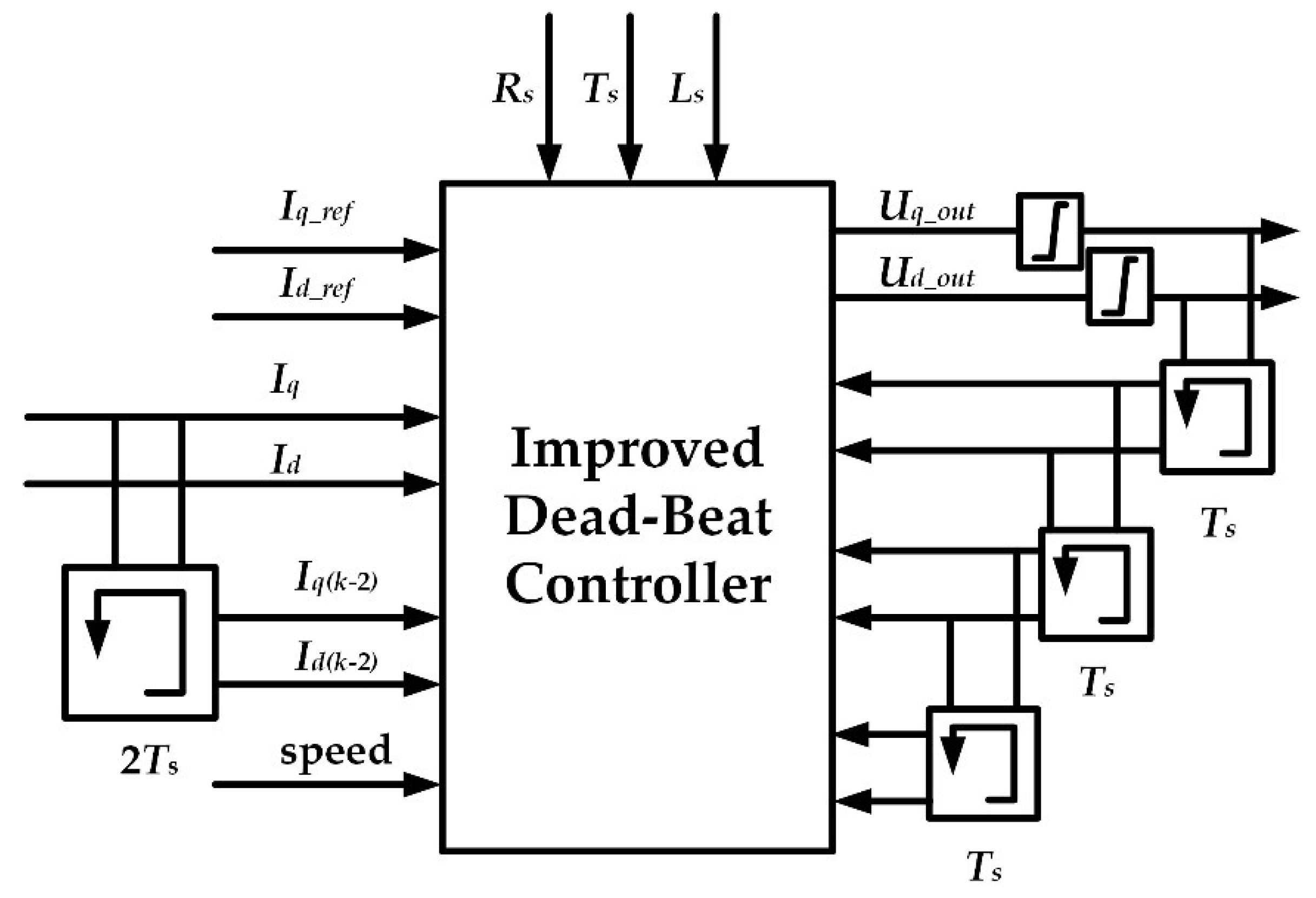
4.1. Proposed Predictive Current Controller

According to the two-beat delay theory and Figure 2, the q-coordinate voltage Equation (2) is discretized by the bilinear discrete method during the T_s from t₁ to t₂, as described below:

$$i_{q(k+1)}=i_{q(k)}+\frac{T_s}{2}\left(\frac{\mathrm{d}{i}_{q(k)}}{\mathrm{d}t}+\frac{\mathrm{d}{i}_{q(k+1)}}{\mathrm{d}t}\right)$$

(14)

Referring to the motor dynamic Equation (2), Equation (14) can be changed to:

$$\frac{i_{q(k+1)}-i_{q(k)}}{T_s}=\frac{1}{2}\left(-\frac{R}{L_s}{i}_{q(k)}+\frac{u_{q(k)}}{L_s}-{\omega }_r{i}_{d(k)}-\frac{{\omega }_r}{L_s}{\psi }_f\right)+\frac{1}{2}\left(-\frac{R}{L_s}{i}_{q(k+1)}+\frac{u_{q(k+1)}}{L_s}-{\omega }_r{i}_{d(k+1)}-\frac{{\omega }_r}{L_s}{\psi }_f\right)$$

(15)

Since the electrical time constant is larger, it is considered conveniently that i_d in (15) remains unchanged for a short time. That is, i_d(k+1) = i_d(k).

During the period from time t₁ to t₂, when considering the discreteness of the digital controller output in the actual situation, the output voltage of the inverter under the ideal condition is kept as the voltage reference value generated at time t₁. In general, the output voltage vector value of the inverter is maintained as the interval start value during each control period T_s. Thus,

$$u_q\left(t\right)=u_{q\left(k\right)}(t_1\le t<t_2)$$

and

$$u_{q(k+1)}=u_{q(k)}$$

(16)

Finally, Equation (15) can be changed to

$$L_s\frac{i_{q(k+1)}-i_{q(k)}}{T_s}=-\frac{R\left(i_{q(k)}+i_{q(k+1)}\right)}{2}+u_{q(k)}-\frac{L_s{\omega }_r\left(i_{d(k)}+i_{d(k+1)}\right)}{2}-{\omega }_r{\psi }_f$$

(17)

During the period of 2T_s from t₁ to t₃, when considering the two-beat delay of the digital current controller, the discretization equation for the q-axis current can be changed to Equation (18) with the same principle as in Equation (17).

$$L_s\frac{i_{q(k+2)}-i_{q(k)}}{T_s}=-R\left(i_{q(k)}+i_{q(k+2)}\right)+\left(u_{q(k)}+u_{q(k+1)}\right)-L_s{\omega }_r\left(i_{d(k)}+i_{d(k+2)}\right)-2{\omega }_r{\psi }_f$$

(18)

Here, the solution process of u_q(k+1) conforms to the mathematical model of PMSM. In theory, the voltage value can adjust the q-coordinate current of motor i_q(k) to the desired value i_qref in two control cycles as follows.

$$\{\begin{array}{l}{i}_{q(k+2)}=i_{qref}\\ i_{d(k+2)}=i_{dref}\end{array}$$

(19)

where u_q(k+1) and u_d(k+1) can be as the reference voltage of the SVPWM module. i_q(k+2) can be the expected reference value of the current.

Substituting Equation (19) into Equation (18), we can get the motor state equation by the bilinear discretization method when considering the two-cycle delay.

$$L_s\frac{i_{qref}-i_{q(k)}}{T_s}=-R\left(i_{q(k)}+i_{qref}\right)+\left(u_{q(k)}+u_{q(k+1)}\right)-L_s{\omega }_r\left(i_{d(k)}+i_{dref}\right)-2{\omega }_r{\psi }_f$$

(20)

For the use of the incremental method, change the discrete interval kT_s~(k + 2)T_s to (k − 2)T_s~kT_s. Like Equation (18), the q-axis discrete voltage equation can be obtained as

$$L_s\frac{i_{q(k)}-i_{q(k-2)}}{T_s}=-R\left(i_{q(k)}+i_{q(k-2)}\right)+\left(u_{q(k-2)}+u_{q(k-1)}\right)-L_s{\omega }_r\left(i_{d(k)}+i_{d(k-2)}\right)-2{\omega }_r{\psi }_f$$

(21)

We can get the result by subtracting Equation (21) from Equation (20) as below.

$$u_{q(k+1)}=\left(R+\frac{L_s}{T_s}\right)\left(i_{qref}-i_{q(k-2)}\right)-\frac{2L_s}{T_s}\left(i_{q(k)}-i_{q(k-2)}\right)-u_{q(k)}+u_{q(k-2)}+u_{q(k-1)}+L_s{\omega }_r\left(i_{dref}-i_{d(k-2)}\right)$$

(22)

Similarly, at the time of (k + 1)T_s, the expected given voltage vector of the d-axis is

$$u_{d(k+1)}=\left(R+\frac{L_s}{T_s}\right)\left(i_{dref}-i_{d(k-2)}\right)-\frac{2L_s}{T_s}\left(i_{d(k)}-i_{d(k-2)}\right)-u_{d(k)}+u_{d(k-2)}+u_{d(k-1)}-L_s{\omega }_r\left(i_{qref}-i_{q(k-2)}\right)$$

(23)

When the improved discretization method is used to discretize the expected voltage equation in the d-q coordinates, it can be seen from (22) and (23) that only the inductance L_s and resistance R of the motor are utilized. In contrast, the traditional predictive control method utilizes parameters such as the permanent magnet flux linkage ψ_f , which will lead to an interference of the controller. The back EMF calculation requires the use of motor speed and other information; the measurement noise can affect these motor parameters, thus deteriorating the system’s performance to some extent.

Moreover, compared with stator resistance and permanent magnet flux linkage, inductance mismatch has a more significant impact on prediction error. It can be seen from Equations (22) and (23) that only a few terms include stator resistance, while the term affected by stator inductance is more. In addition, considering that the magnitude of rotational speed is much larger than that of stator resistance and I_d, I_q, the terms which include L_s would affect the final values of u_d and u_q. Therefore, the control scheme can be easily used in actual applications.

4.2. Stability Analysis of Control Algorithm

The stable condition of the deadbeat predictive control can be derived from the discrete relationship between the actual current value and the given value. Assuming that current control is stable in two sampling periods: $i_{q(k+2)}=i_{q(k+2)}^{*}$, $i_{d(k+2)}=i_{d(k+2)}^{*}$, then Equations (22) and (23) can be expressed as:

$$u_{d(k+1)}^{*}=\left(R_0+\frac{L_0}{T_s}\right)\left(i_{d(k+2)}^{*}-i_{d(k-2)}\right)-\frac{2L_0}{T_s}\left(i_{d(k)}-i_{d(k-2)}\right)-u_{d(k)}+u_{d(k-2)}+u_{d(k-1)}-L_0{\omega }_r\left(i_{q(k+2)}^{*}-i_{q(k-2)}\right)$$

(24)

$$u_{q(k+1)}^{*}=\left(R_0+\frac{L_0}{T_s}\right)\left(i_{q(k+2)}^{*}-i_{q(k-2)}\right)-\frac{2L_0}{T_s}\left(i_{q(k)}-i_{q(k-2)}\right)-u_{q(k)}+u_{q(k-2)}+u_{q(k-1)}+L_0{\omega }_r\left(i_{d(k+2)}^{*}-i_{d(k-2)}\right)$$

(25)

where L₀ and R₀ are the nominal parameters of the motor.

When the actual parameters L and R of the motor are brought into the controller, the actual control voltage for the d-q axis in the deadbeat prediction control is:

$$u_{d(k+1)}^{}=\left(R_0+\frac{L_0}{T_s}\right)\left(i_{d(k+2)}^{}-i_{d(k-2)}\right)-\frac{2L_0}{T_s}\left(i_{d(k)}-i_{d(k-2)}\right)-u_{d(k)}+u_{d(k-2)}+u_{d(k-1)}-L_0{\omega }_r\left(i_{q(k+2)}^{}-i_{q(k-2)}\right)$$

(26)

$$u_{q(k+1)}^{}=\left(R_0+\frac{L_0}{T_s}\right)\left(i_{q(k+2)}^{}-i_{q(k-2)}\right)-\frac{2L_0}{T_s}\left(i_{q(k)}-i_{q(k-2)}\right)-u_{q(k)}+u_{q(k-2)}+u_{q(k-1)}+L_0{\omega }_r\left(i_{d(k+2)}^{}-i_{d(k-2)}\right)$$

(27)

The desired voltage in Equations (24) and (26) should be: $u_{d(k+1)}=u_{d(k+1)}^{*}$, and the voltage in Equations (25) and (27) should be: $u_{q(k+1)}=u_{q(k+1)}^{*}$. Thus, the relationship between the reference current and the actual value of the current can be derived as follows:

$$i_{d(k+2)}\left(R+\frac{L}{T_s}\right)-i_{d(k+2)}^{*}\left(R_0+\frac{L_0}{T_s}\right)-i_{d(k-2)}\left(\left(R-R_0\right)-\frac{L-L_0}{T_s}\right)-i_{d(k)}\frac{2\left(L-L_0\right)}{T_s}-\left(L-L_0\right){\omega }_r(i_{q(k+2)}-i_{q(k-2)})=0$$

(28)

$$i_{q(k+2)}\left(R+\frac{L}{T_s}\right)-i_{q(k+2)}^{*}\left(R_0+\frac{L_0}{T_s}\right)-i_{q(k-2)}\left(\left(R-R_0\right)-\frac{L-L_0}{T_s}\right)-i_{q(k)}\frac{2\left(L-L_0\right)}{T_s}+\left(L-L_0\right){\omega }_r(i_{d(k+2)}-i_{d(k-2)})=0$$

(29)

Considering that the sampling time T_s is small enough, multiply T_s at both sides of Equations (28) and (29), and then let T_s = 0, we have

$$i_{d(k+2)}L-i_{d(k+2)}^{*}{L}_0+i_{d(k-2)}\left(L-L_0\right)=i_{d(k)}2\left(L-L_0\right)$$

(30)

$$i_{q(k+2)}L-i_{q(k+2)}^{*}{L}_0+i_{q(k-2)}\left(L-L_0\right)=i_{q(k)}2\left(L-L_0\right)$$

(31)

When T_s = 0 (T_s is small enough) and $i_{d(k+2)}^{*}=0$ (a kind of control strategy makes i_d = 0), the back EMF is considered as a disturbance in the current loop.

$$\frac{L}{L_0}{i}_{d(k+2)}+\frac{L}{L_0}{i}_{d(k-2)}-2\frac{L}{L_0}{i}_{d(k)}=-2i_{d(k)}+i_{d(k-2)}$$

(32)

$$i_{q(k+2)}\frac{L}{L_0}+i_{q(k-2)}\frac{L}{L_0}-2i_{q(k)}\frac{L}{L_0}=-2i_{q(k)}+i_{q(k-2)}+i_{q(k+2)}^{*}$$

(33)

Performing the z-transform on Equations (30) and (31), the discrete-domain closed-loop transfer function between the current preset value and the actual value is:

$$\frac{i_{x(z)}}{i_{x(z)}^{*}}=\frac{z^4}{\frac{L}{L_0}{\left(z^2-1\right)}^2+2\left(z^2-1\right)+1}$$

(34)

where x = d or q.

Letting X = z² − 1, the denominator of Equation (34) is changed to $\frac{L}{L_0}{\left(X\right)}^2+2X+1$. So, the roots of equation $Y\left(X\right)=\frac{L}{L_0}{\left(X\right)}^2+2X+1$ correspond to the system poles. The condition of the poles inside the unit circle corresponds to the condition of the system stability. If L₀ = L, the transfer function in Equation (34) will be equal to one, which is trivial. In the following, only the cases of L₀ > L and L₀ < L are considered.

• L₀ > L

When L₀ > L, the quadratic equation Y(X) has two real solutions which are

$$X_{1,2}=-\frac{L_0}{L}\pm \frac{L_0}{L}\sqrt{1-\frac{L}{L_0}}$$

(35)

Then, we get $z_{1,2}^2=\left(1-\frac{L_0}{L}\right)\pm \sqrt{\frac{L_0}{L}\left(\frac{L_0}{L}-1\right)}$. Let $m=\frac{L_0}{L}-1$ which is always big than 0. Thus, $z_{1,2}^2=-m\pm \sqrt{m\left(m+1\right)}$. With respect to z₁, we can get

$$\left|z_1^2\right|=\left|-m+\sqrt{m\left(m+1\right)}\right|=\frac{m}{m+\sqrt{m\left(m+1\right)}}<1,$$

and with respect to z₂, we can get

$$\left|z_2^2\right|=\left|-m-\sqrt{m\left(m+1\right)}\right|=\frac{1}{\sqrt{1+\frac{1}{m}}-1}$$

It is easy to show that $\left|z_2^2\right|<1$ when 0 < m < 1/3. That is L₀ > L > 3L₀/4. To this end, the system is stable when L₀ > L > 3L₀/4.

• L₀ < L

When L₀ < L, X will have imaginary solutions, which are:

$$X_{1,2}=\frac{-b\pm \left(\sqrt{4ac-b^2}\right)\mathrm{j}}{2a}=\frac{L_0}{L}\left[-1\pm \left(\sqrt{{\frac{L}{L}}_0-1}\right)\mathrm{j}\right]$$

(36)

According to the assumed condition X = z² − 1, we can get

$$z^2=\frac{L_0}{L}\left[-1\pm \left(\sqrt{\frac{L}{L_0}-1}\right)\mathrm{j}\right]+1=\left(1-\frac{L_0}{L}\right)\pm \left(\sqrt{\frac{L_0}{L}-{\left(\frac{L_0^{}}{L}\right)}^2}\right)\mathrm{j}$$

(37)

Assuming z = d − ej, we can get

$$\{\begin{array}{l}{d}^2-e^2=1-\frac{L_0}{L}\\ 2de=\pm \sqrt{\frac{L_0}{L}-{\left(\frac{L_0^{}}{L}\right)}^2}\end{array}$$

(38)

where d and e are real numbers. By solving Equation (38), we can get

$$d^4-\left(1-\frac{L_0}{L}\right)d^2+\frac{L_0^2}{4L^2}\left(1-\frac{L}{L_0}\right)=0$$

(39)

$$e^4+\left(1-\frac{L_0}{L}\right)e^2+\frac{L_0^2}{4L^2}\left(1-\frac{L}{L_0}\right)=0$$

(40)

The condition that the controller is stable when |Z| < 1, which is equivalent to d² + e² < 1. From Equations (39) and (40), it is easy to have

$$d^2{}_{1,2}=\frac{(1-\frac{L_0}{L})+\left(\sqrt{1-\frac{L_0}{L}}\right)}{2}$$

(41)

$$e^2{}_{1,2}=\frac{-(1-\frac{L_0}{L})+\left(\sqrt{1-\frac{L_0}{L}}\right)}{2}$$

(42)

It is obvious that d² + e² < 1. Therefore, the system under the controller is constantly stable, when L₀ < L.

Based on the analysis above, it can be concluded that the closed-loop system is stable when L > (3/4) L₀. We will assume this condition in this paper.

5. Simulation and Experiment Validation

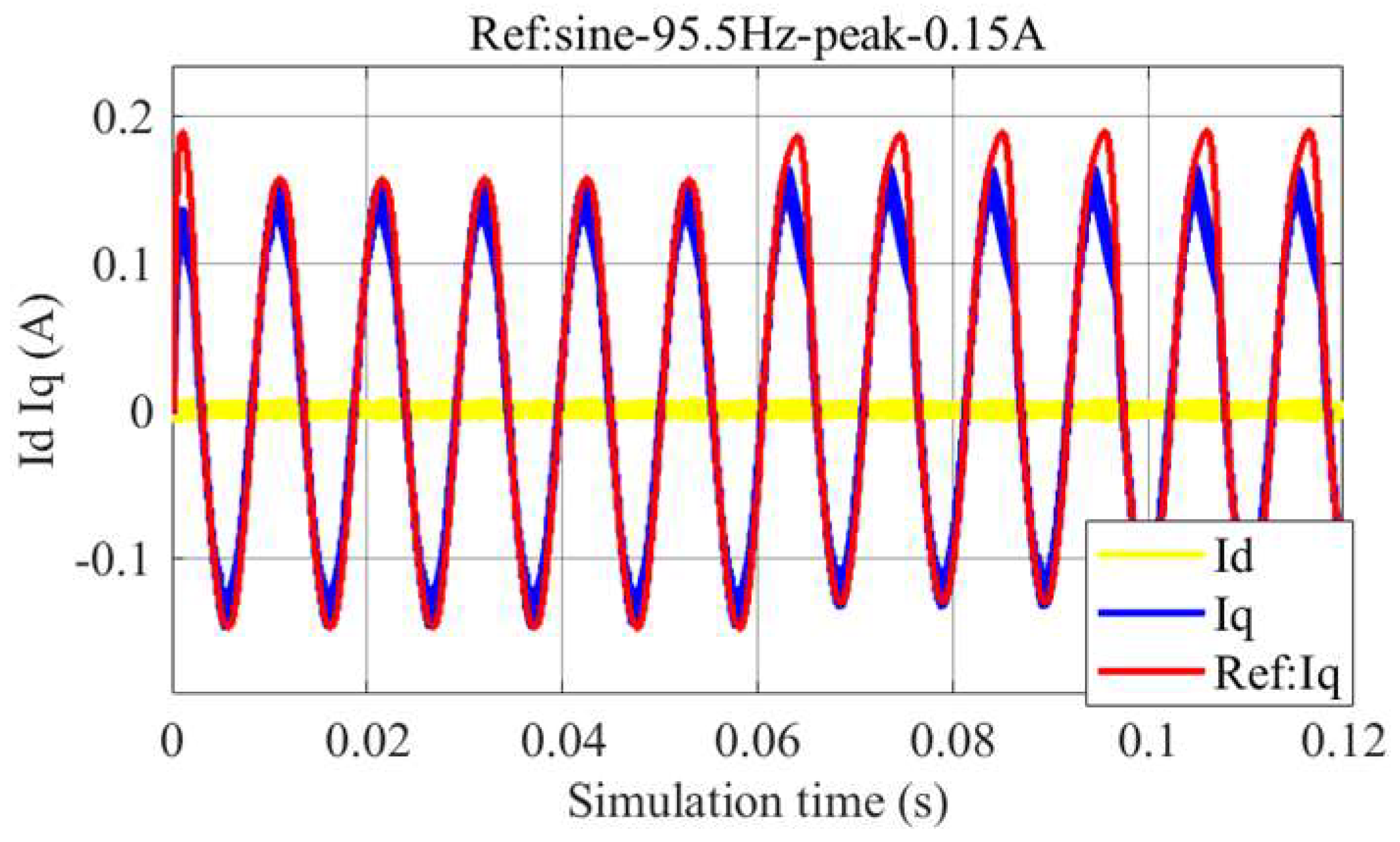
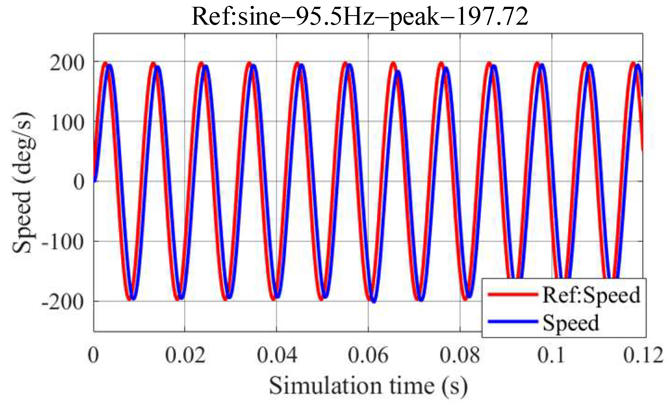
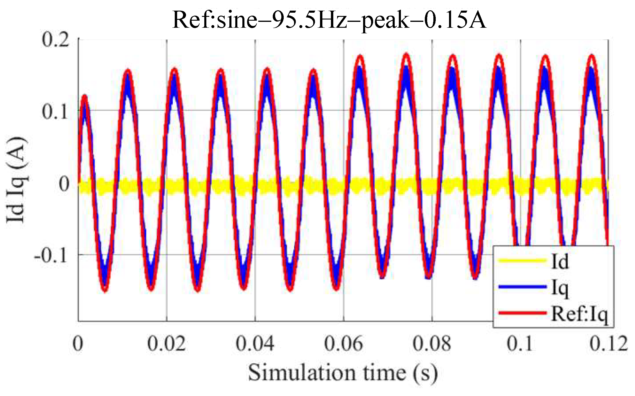
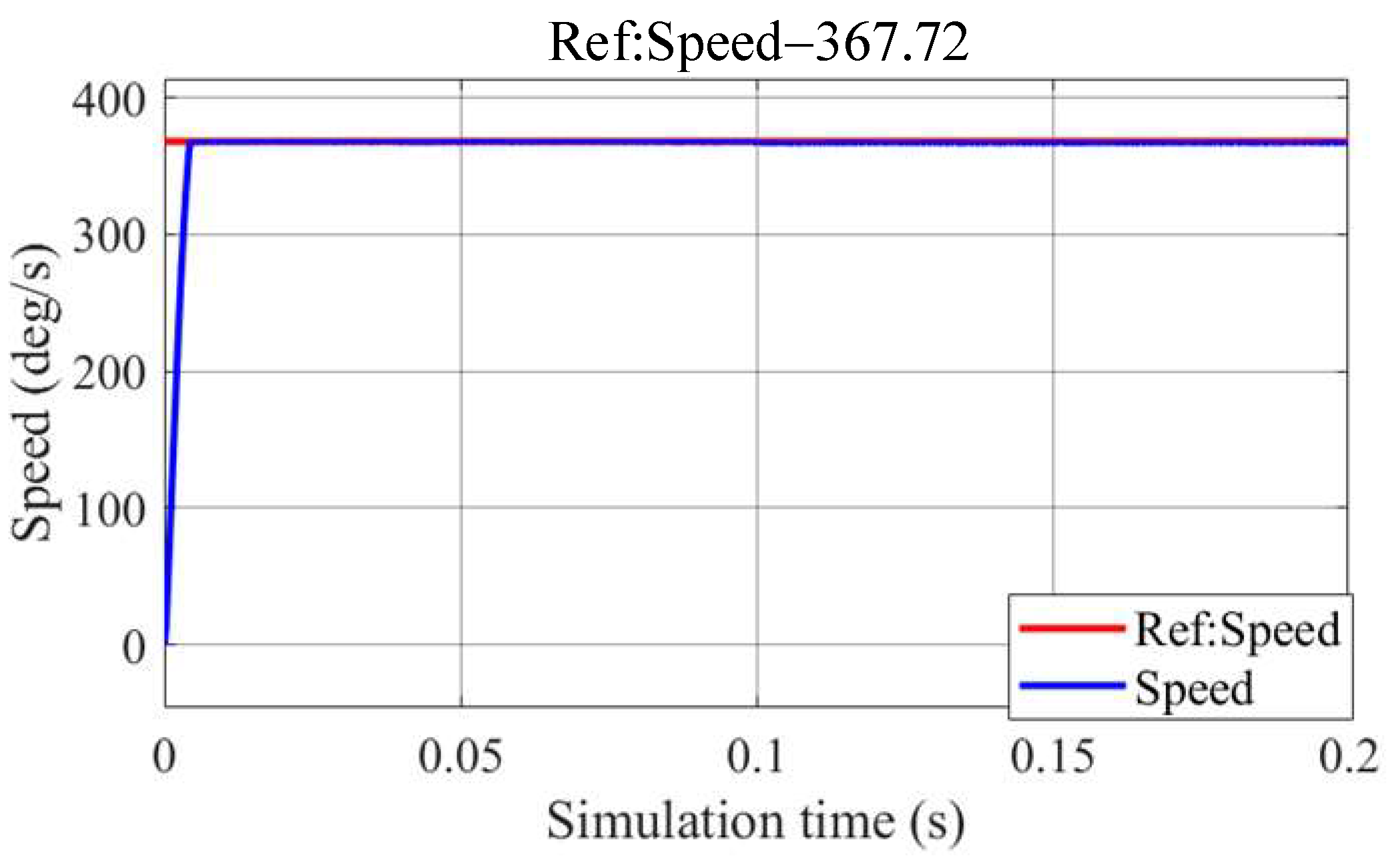
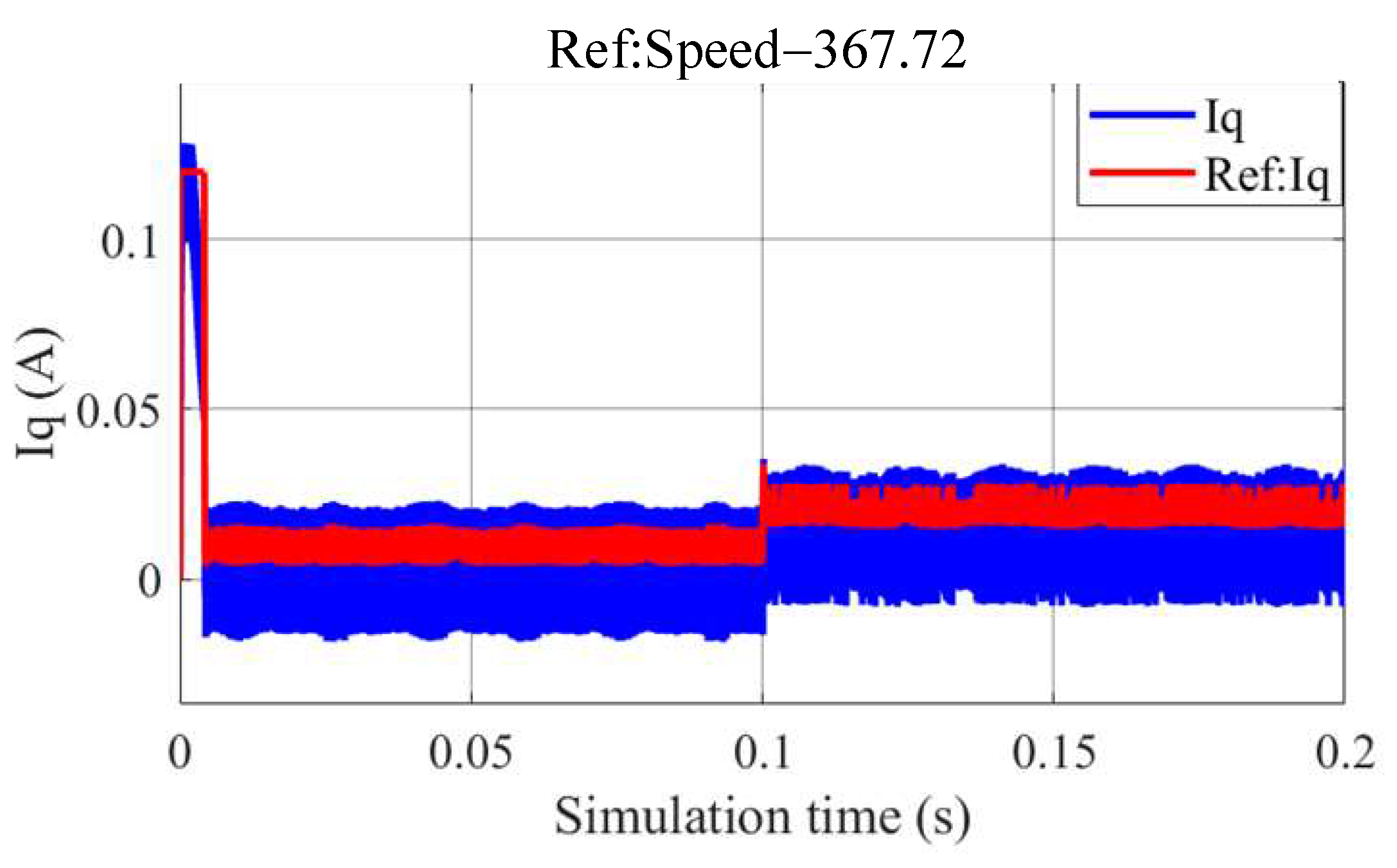
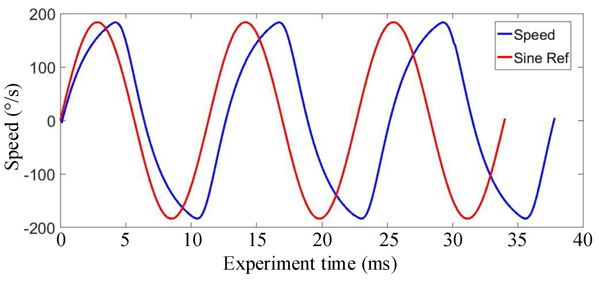
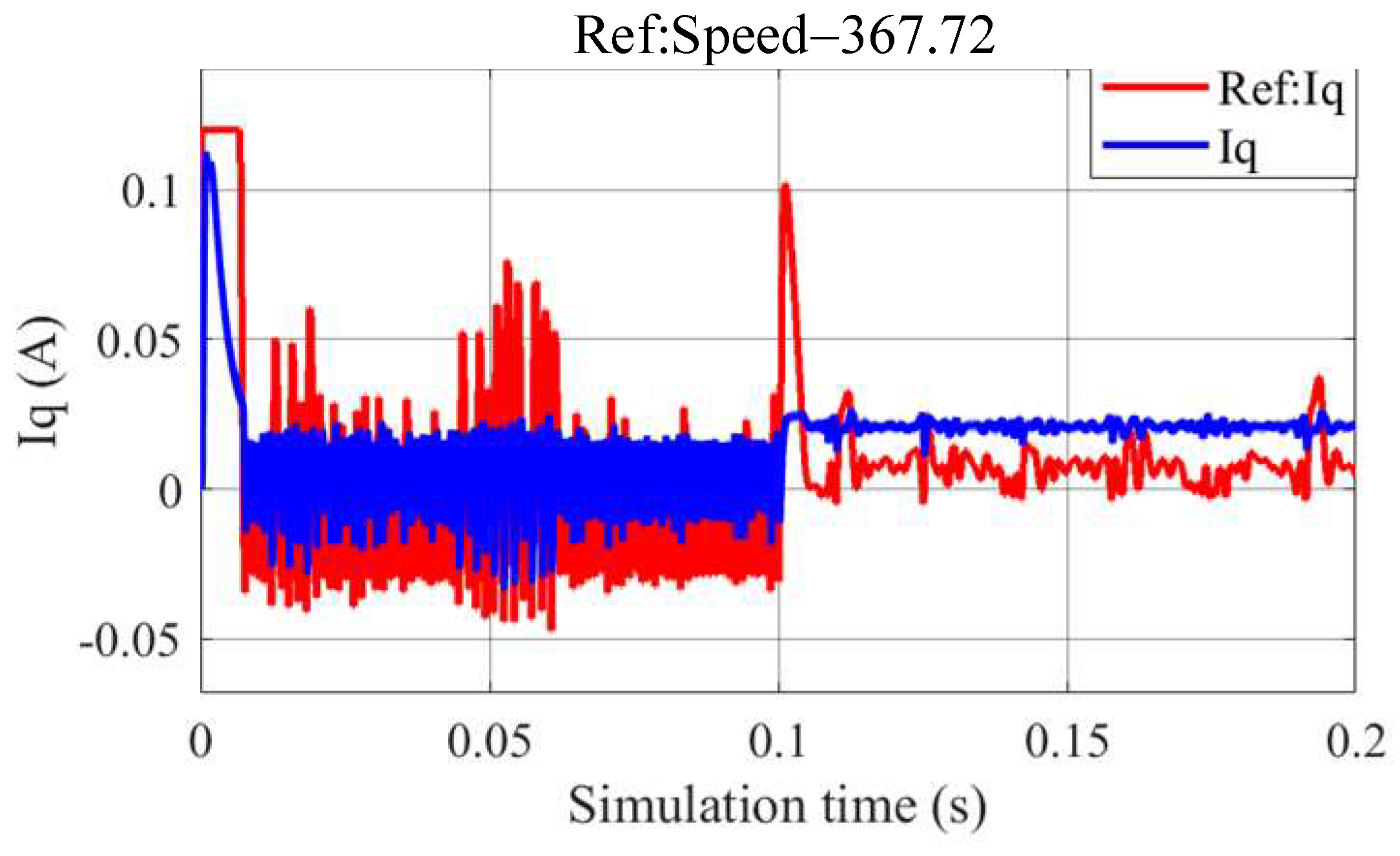
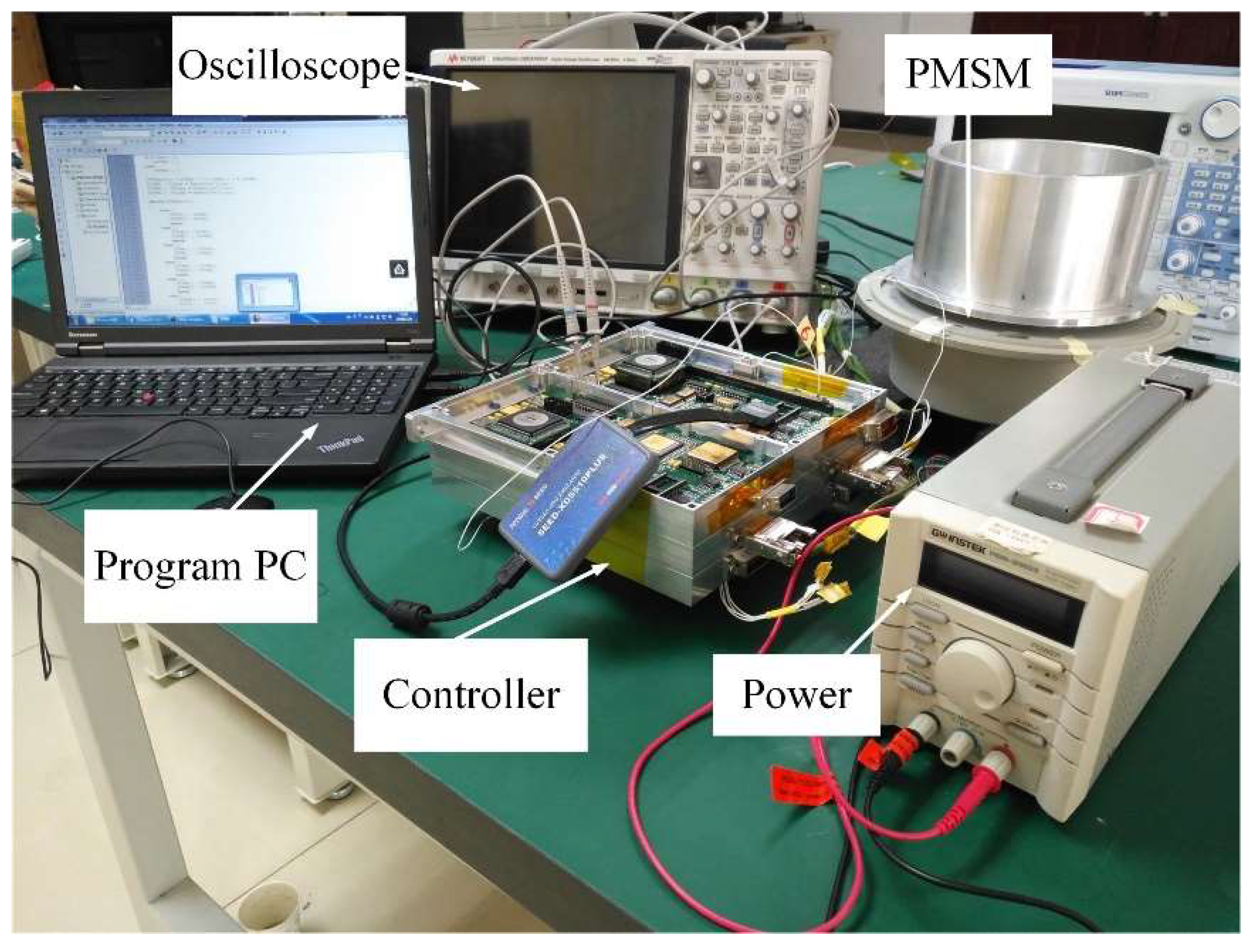
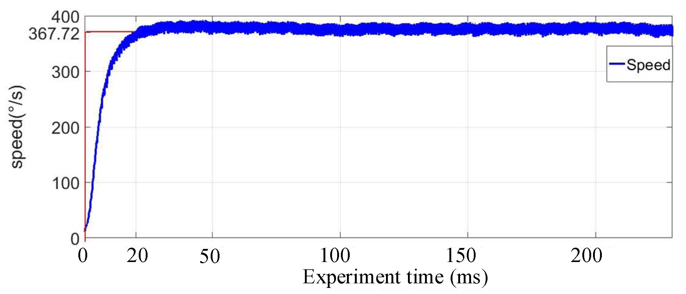
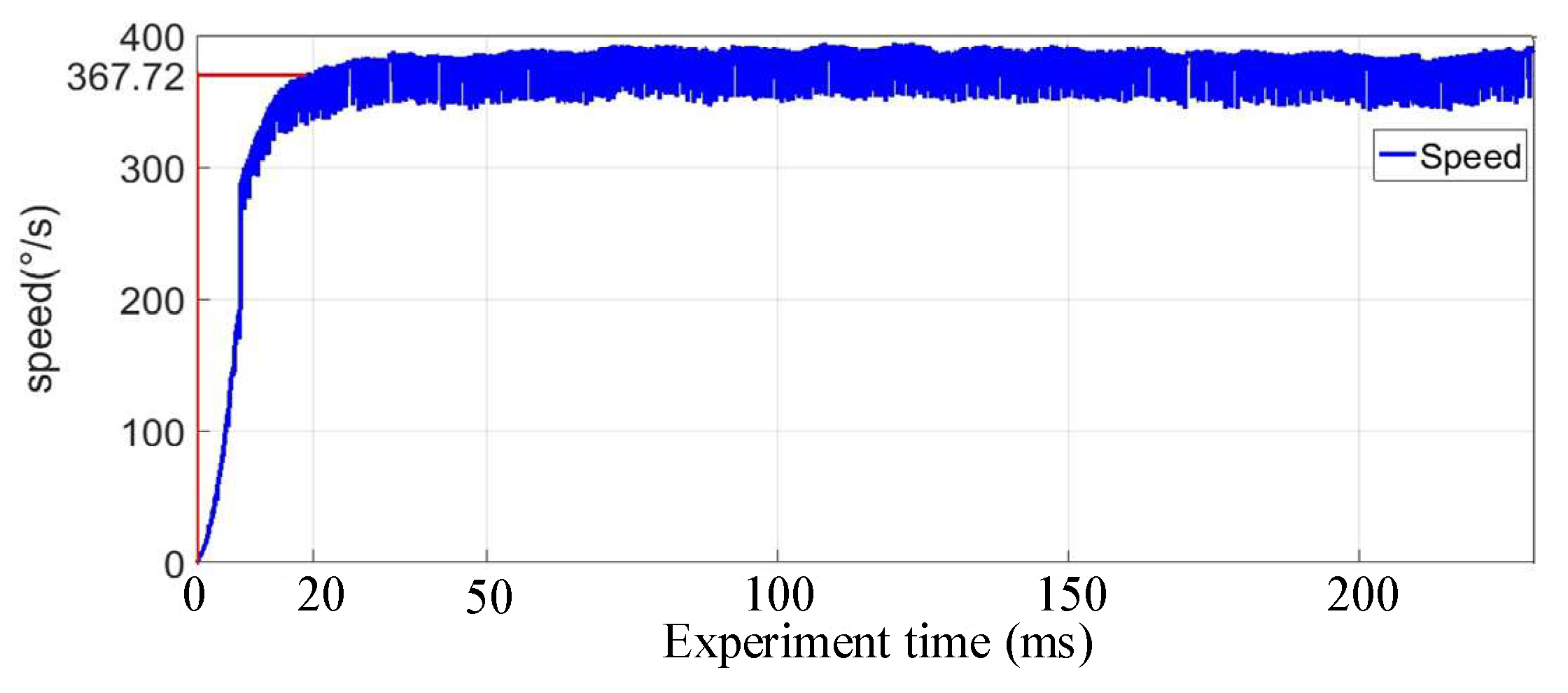
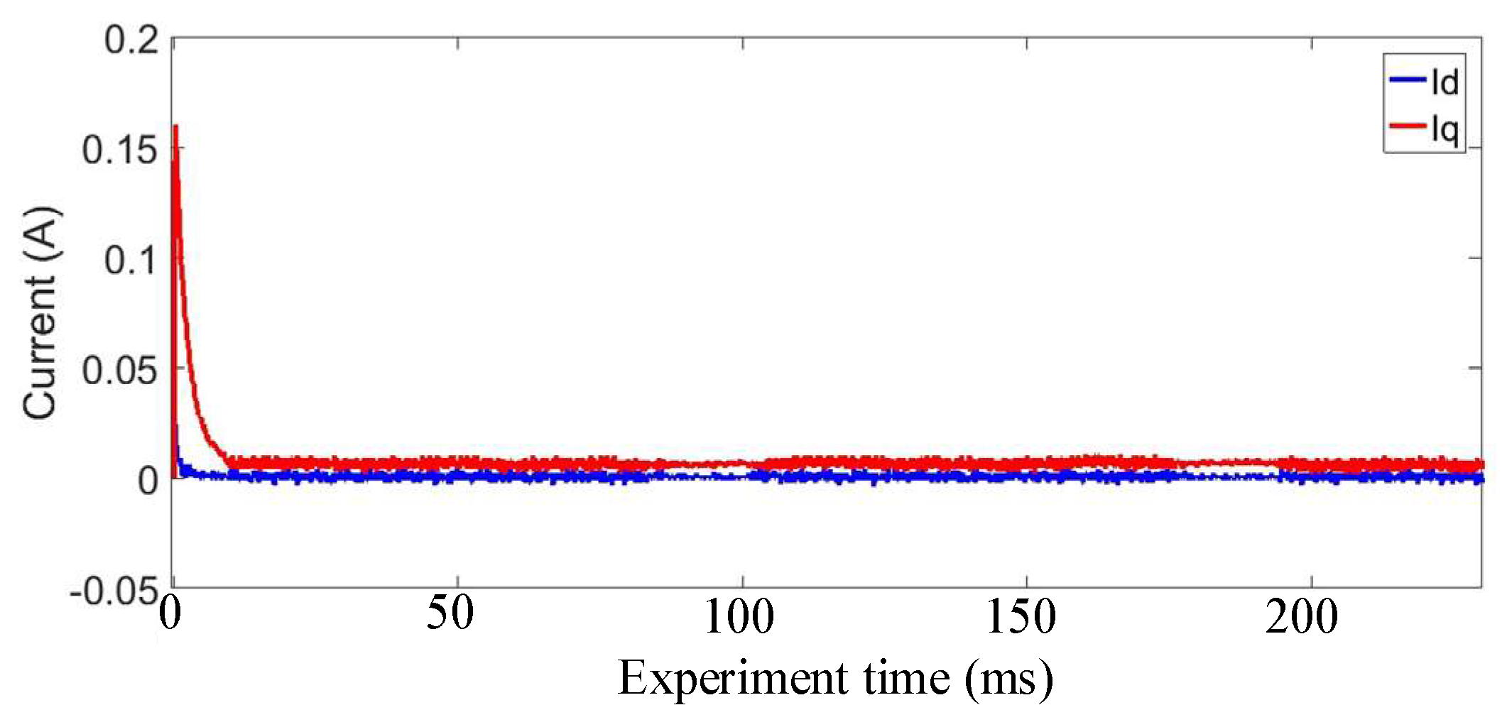
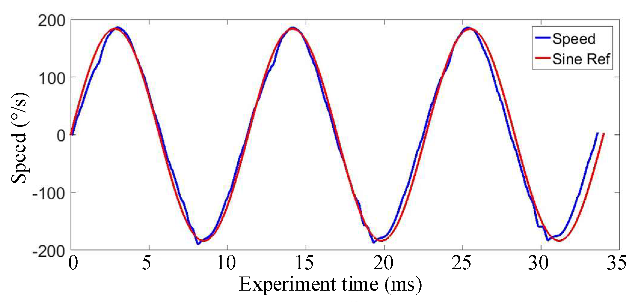
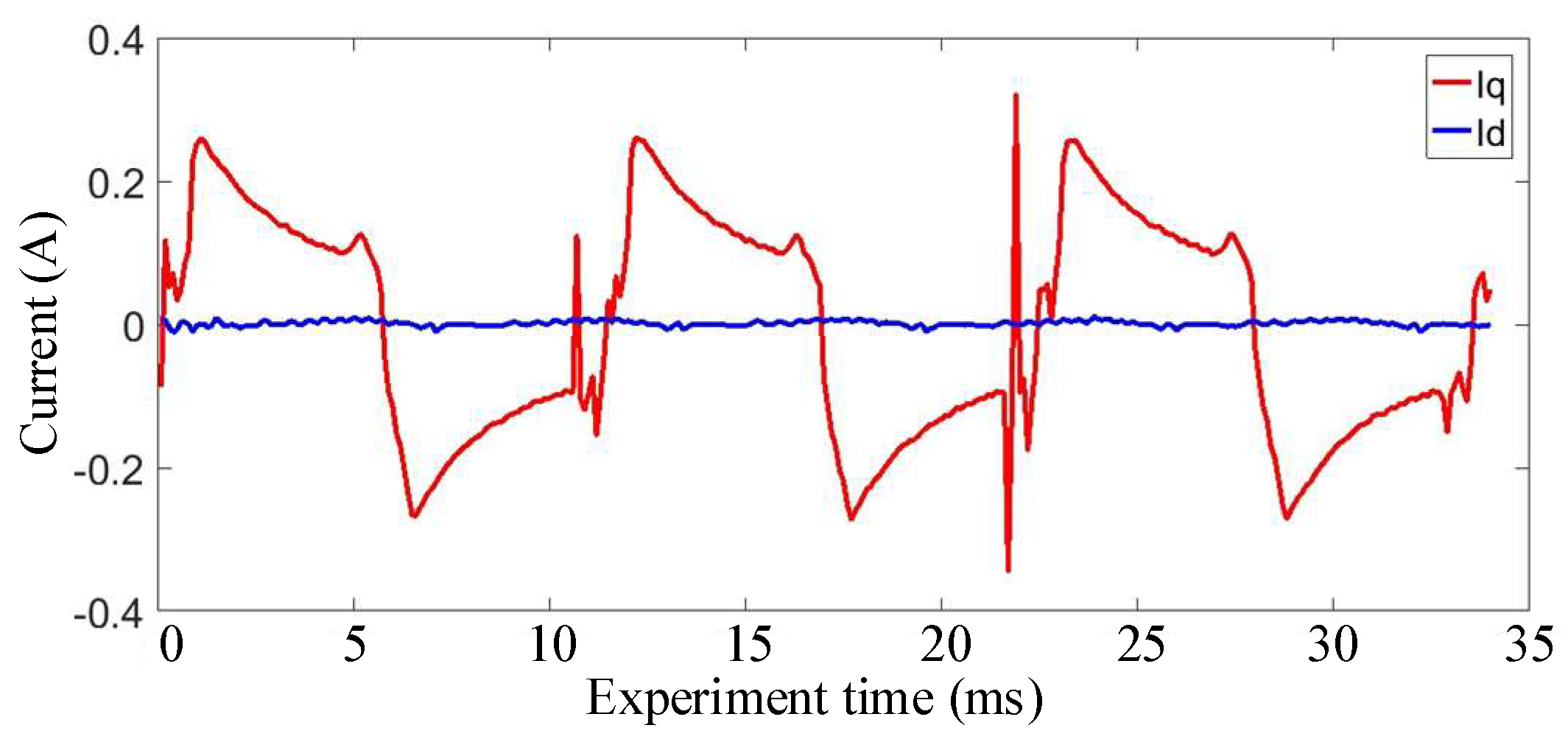
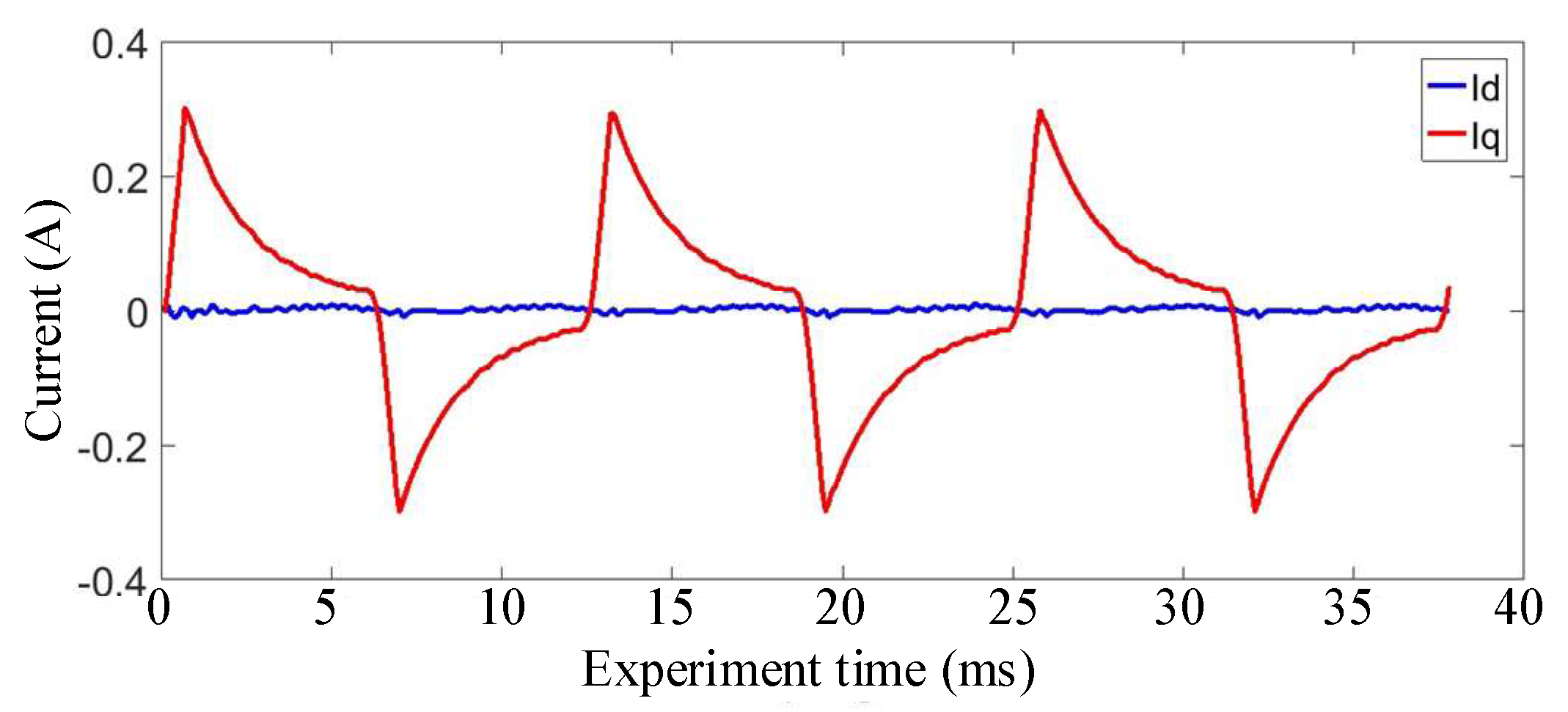
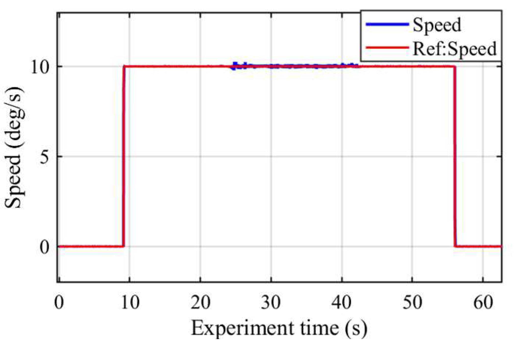
In this section, the simulation and experimental results of the proposed predictive current algorithm are shown. The motor parameters in both simulation and experiment are the same, as shown in

Table 1. Motor parameters in both simulation and experiment.

Parameter	Unit	Value
Stator resistance R	Ω	48.9
Inductance Ld = Lq	H	14 × 10−3
Number of poles p		10
Inertial J	kg·m2	9.717 × 10−5
Torque constant	N*m/A_peak	1.4213

.

The simulation is based on MATLAB/Simulink. The practical experiment is based on a platform that contains TMS320C6701 (DSP) and A54SX72A (FPGA). The current control frequency in both the simulation and practical experiment is 10 kHz.

The speed loop applies a PI controller in both simulations and experiments. The parameters of the PI controller in all experiments are the same to evaluate the performance of different current control strategies.

5.1. Simulation

The scheme of the improved deadbeat current controller in the simulation is shown in Figure 3. The memory module in Simulink is used to save the calculation results and retrieve the values obtained in the previous cycle. The reference value of the current in Figure 3 is the output value of the speed controller. As the inverter cannot output overlarge voltage in practical systems, the command voltage calculated from the predictive model must be restricted. Based on amplitude coordinate transformation, the maximum output voltage in the synchronous rotating coordinate is 2/3U_dc.

The switching frequency of the PWM inverter is set to 10 kHz (reload every second period). The sampling period is 20 µs. In the simulation, the parameters for the system are summarized in

Table 2. Simulation Parameters.

Simulation Parameter	Value
$\mathrm{DC}\mathrm{Bus}\mathrm{Voltage}{U}_{dc}$	28 V
Triangular Carrier Frequency	10 kHz
Triangular Carrier Output	[0 1250 0]
Simulation Solver	Runge-Kutta
Rated Speed	367.72 deg/s
Step Size	10−7

.

When the system uses a PI controller as the speed controller and the proposed controller as the current controller, the simulation results of rotational speed and the current in d-q coordinates are shown in Figure 4 and Figure 5. The speed reference in the simulation is a sine wave with an amplitude of 197.72 degrees per second and a frequency of 95.5 Hz. Although such a high frequency is not needed on actual satellites, we want to achieve the highest possible frequency when doing research to verify our control performance. Moreover, the bandwidth would be affected when there is a reducer. In actual satellite, a sine speed control signal is often used for the CMG frame control system. During the start-up of the motor, the control system is unloaded until the rotor speed is stable and the simulation time is more than half. The same simulation is performed using a conventional deadbeat current controller with all the system parameters remaining unchanged. The simulation results are shown in Figure 6 and Figure 7.

Comparing the speed results and the detailed view in Figure 4 and Figure 6, both the conventional deadbeat current controller and the proposed improved deadbeat current controller can be combined with the PI speed controller. The rotor speed can quickly follow the given value when the motor starts without load. The system can accurately track the reference and remain stable with the rated load during the sine sweep operation. It can be seen from the speed curve that the steady-state performance of the system with the improved deadbeat current controller seems to be better. From the simulation results, in general, both current controllers show good dynamic response and stability.

From the current of the d-q coordinates in Figure 5 and Figure 7, the improved deadbeat controller has a better dynamic current response under the same conditions. The q-axis current I_q follows the current reference Ref: I_q. However, there is a phase deviation between the output current and the reference when the conventional controller is adopted.

Keeping the system parameters unchanged, the speed reference is changed from sine to step. Under the same simulation environment and parameters, the dynamic response performance of the current controller is verified. At 0.01 s during the simulation, the given speed is stepped from 0 to 367.72 degrees per second. At 0.03 s during the simulation, a rated load of 0.0296 N is brought into the servo system.

When the improved deadbeat current controller proposed in this paper is used, the simulation results are shown in Figure 8 and Figure 9. Figure 8 shows the speed waveform which contains start-up process without load and dynamic loading of the servo system. Figure 9 shows the current waveform in the q-coordinate following the output value of the speed controller under the same conditions. Under the same conditions as a conventional deadbeat controller, the simulation results are shown in Figure 10 and Figure 11.

By comparing the speed waveforms in Figure 8 and Figure 10, it can be seen that the rotor speed with the improved controller can track the given step quickly and keep a small steady-state error. By comparing the q-axis current waveforms in Figure 9 and Figure 11, it is shown that the proposed improved deadbeat current prediction controller has a better current tracking performance than the conventional controller.

5.2. Experiments

The motor parameters used in the simulation are consistent with the nominal values of the actual motor. The motor is operated without load according to demand. The platform used in the experiment is shown in Figure 12, including the inertia load, computer, 28 V DC power supply and controller. The controller’s interrupt time and sampling time are consistent with the simulation design. The experimental results record the waveform of the motor’s speed and q- coordinate current.

When the given speed is 367.72 degrees per second, the dynamic start-up process of the motor and the static rotation state are recorded. Figure 13 and Figure 14 show the motor speed with the improved deadbeat current controller and the conventional deadbeat current controller, respectively. Figure 15 and Figure 16 show the motor current in d-q coordinates with the improved deadbeat current controller and the conventional deadbeat current controller, respectively.

When the speed reference value is the sine waveform with a certain amplitude and a certain frequency, the speed curve of the servo system with the improved deadbeat current controller is shown in Figure 17. Figure 18 shows the motor current in d-q coordinates. When the traditional controller is used and the speed reference is sine, the speed curve is shown in Figure 19, and the motor current in d-q coordinates are shown in Figure 20.

Based on the speed curves shown in Figure 17 and Figure 19, it is found that the improved deadbeat current controller has a significant performance improvement over the conventional deadbeat current controller when tracking sinusoidal speeds. The phase delay problem occurs in the sinusoidal speed by the traditional deadbeat controller. In the actual satellite maneuvering process, the CMG frame motor is controlled according to the sine waveform to avoid impact on the satellite. So, the proposed controller has a good application.

This PMSM is installed on an actual CMG frame control platform (the main parameters of the platform are 50 Nms CMG, the maximum output torque is 50 Nm, and the maximum speed is 72°/s), and the experiment with imposed load torque is carried out. Since the PMSM drives the frame through the reducer, the speed given in the experiment is 10°/s. The experiment results are shown in Figure 21 and Figure 22. As can be seen from the figures, the CMG framework can be well controlled by the control method proposed in this paper, and the control effect of the motor current is very good.

6. Conclusions

A novel incremental deadbeat current prediction control algorithm based on the bilinear discretization mathematical model of the PMSM is proposed in this paper. To establish a high precision mathematical model of the PMSM, two-beat delay of the digital system has been considered, and delay compensation has been made. The PMSM control system can be achieved at fast and precise current control with constant switching frequency and low current ripple. Moreover, delay compensation improves the accuracy of the control system model and makes the system more stable. The simulation and experimental results demonstrate that the digital controlled system can achieve high dynamic current response and low current ripple. The new model and control algorithm are of great use for CMG.

References

- Kwon, Y.; Kim, S.; Sul, S. Six-step operation of PMSM with instantaneous current control. IEEE Trans. Ind. Appl. 2014, 50, 2614–2625. [Google Scholar] [CrossRef]
- Hezzi, A.; Ben Elghali, S.; Bensalem, Y.; Zhou, Z.; Benbouzid, M.; Abdelkrim, M.N. ADRC-based robust and resilient control of a 5-phase PMSM driven electric vehicle. Machines 2020, 8, 17. [Google Scholar] [CrossRef]
- Wang, C.; Chen, M.; Hu, B.; Yan, L.; Yu, Y.; Zou, J.; Guo, Y.; Li, G. Design of high reliability gimbal servo system of control moment gyroscope. In Proceedings of the 2019 IEEE 2nd International Conference on Information Systems and Computer Aided Education (ICISCAE), Dalian, China, 23–30 September 2019; pp. 442–445. [Google Scholar]
- Mao, H.; Yang, X.; Chen, Z.; Wang, Z. A hysteresis current controller for single-phase three-level voltage source inverters. IEEE Trans. Power Electron. 2012, 27, 3330–3339. [Google Scholar] [CrossRef]
- Dey, A.; Rajeevan, P.P.; Ramchand, R.; Mathew, K.; Gopakumar, K. A space-vector-based hysteresis current controller for a general n-level inverter-fed drive with nearly constant switching frequency control. IEEE Trans. Ind. Electron. 2013, 60, 1989–1998. [Google Scholar] [CrossRef]
- Lee, J.S.; Lorenz, R.D. Deadbeat direct torque and flux control of IPMSM drives using a minimum time ramp trajectory method at voltage and current limits. IEEE Trans. Ind. Appl. 2012, 50, 3795–3804. [Google Scholar] [CrossRef]
- Gabbi, T.S.; Grundling, H.A.; Vieira, R.P. Current controller for sensorless PMSM drive using combined sliding mode strategy and disturbance observer. In Proceedings of the 41st Annual Conference of the IEEE Industrial Electronics Society, Yokohama, Japan, 9–12 November 2015; pp. 3773–3778. [Google Scholar]
- Hou, Q.; Ding, S.; Yu, X. Composite super-twisting sliding mode control design for PMSM speed regulation problem based on a novel disturbance observer. IEEE Trans. Energy Convers. 2020, 36, 2591–2599. [Google Scholar] [CrossRef]
- Kazmierkowski, M.P.; Malesani, L. Current control techniques for three-phase voltage-source PWM converters: A survey. IEEE Trans. Ind. Electron. 1998, 45, 691–703. [Google Scholar] [CrossRef]
- Rowan, T.M.; Kerkman, R.J. A new synchronous current regulator and an analysis of current-regulated PWM inverters. IEEE Trans. Ind. Appl. 1986, 22, 678–690. [Google Scholar] [CrossRef]
- Song, W.; Ma, J.; Zhou, L.; Feng, X. Deadbeat predictive power control of single-phase three-level neutral-point-clamped converters using space-vector modulation for electric railway traction. IEEE Trans. Power Electron. 2016, 31, 721–731. [Google Scholar] [CrossRef]
- Liu, Q.; Chang, X. Position IP control of a permanent magnet synchronous motor based on fuzzy neural network. In Proceedings of the 2018 Chinese Control And Decision Conference (CCDC), Shenyang, China, 9–11 June 2018; pp. 1081–1086. [Google Scholar]
- Moon, H.T.; Kim, H.S.; Youn, M.J. A discrete-time predictive current control for PMSM. IEEE Trans. Power Electron. 2003, 18, 464–472. [Google Scholar] [CrossRef]
- Morel, F.; Lin-Shi, X.; Retif, J.-M.; Allard, B.; Buttay, C. A comparative study of predictive current control schemes for a permanent-magnet synchronous machine drive. IEEE Trans. Ind. Electron. 2009, 56, 2715–2728. [Google Scholar] [CrossRef] [Green Version]
- Liu, H.; Li, S. Speed control for PMSM servo system using predictive functional control and extended state observer. IEEE Trans. Ind. Electron. 2012, 59, 1171–1183. [Google Scholar] [CrossRef]
- Preindl, M.; Schaltz, E. Sensorless model predictive direct current control using novel second-order PLL observer for PMSM drive systems. IEEE Trans. Ind. Electron. 2011, 58, 4087–4095. [Google Scholar] [CrossRef]
- Xie, W.; Wang, X.C.; Wang, F.X.; Xu, W.; Kennel, R.M.; Gerling, D.; Lorenz, R.D. Finite control set-model predictive torque control with a deadbeat solution for PMSM drives. IEEE Trans. Ind. Electron. 2015, 62, 5402–5410. [Google Scholar] [CrossRef]
- Zhang, X.G.; Hou, B.S.; Mei, Y. Deadbeat predictive current control of permanent magnet synchronous motors with stator current and disturbance observer. IEEE Trans. Power Electron. 2017, 32, 3818–3834. [Google Scholar] [CrossRef]
- Tong, L.; Zou, X.D.; Feng, S.S.; Chen, Y.; Kang, Y.; Huang, Q.J.; Huang, Y.R. An SRF-PLL-based sensorless vector control using the predictive deadbeat algorithm for the direct-driven permanent magnet synchronous generator. IEEE Trans. Power Electron. 2014, 29, 2837–2849. [Google Scholar] [CrossRef]
- Malesani, L.; Mattavelli, P.; Buso, S. Robust dead-beat current control for PWM rectifiers and active filters. IEEE Trans. Ind. Appl. 1999, 35, 613–620. [Google Scholar] [CrossRef]
- Cortes, P.; Rodriguez, J.; Silva, C.; Flores, A. Delay compensation in model predictive current control of a three-phase inverter. IEEE Trans. Ind. Electron. 2012, 59, 1323–1325. [Google Scholar] [CrossRef]
- Moreno, J.; Huerta, J.; Gil, R.; Gonzalez, S. A robust predictive current control for three-phase grid-connected inverters. IEEE Trans. Ind. Electron. 2009, 56, 1993–2004. [Google Scholar] [CrossRef]
- Zhang, Y.; Zhu, J.; Xu, W. Analysis of one step delay in direct torque control of permanent magnet synchronous motor and its remedies. In Proceedings of the 2010 International Conference on Electrical Machines and Systems, Incheon, Korea, 10–13 October 2010; pp. 792–797. [Google Scholar]
- Barros, J.D.; Silva, J.F.A.; Jesus, E.G.A. Fast predictive optimal control of NPC multilevel converters. IEEE Trans. Ind. Electron. 2013, 60, 619–627. [Google Scholar] [CrossRef]
- Shi, Y.; Sun, K.; Huang, L.; Li, Y. Online identification of permanent magnet flux based on extended Kalman filter for IPMSM drive with position sensorless control. IEEE Trans. Ind. Electron. 2012, 59, 4169–4178. [Google Scholar] [CrossRef]