Article

Path Planning Strategy for a Manipulator Based on a Heuristically Constructed Network

1
School of Automation, Beijing University of Posts and Telecommunications, Beijing 100876, China
2
Beijing Key Laboratory of Intelligent Space Robotic System Technology and Applications, Institute of Spacecraft System Engineering, Beijing 100094, China
*
Author to whom correspondence should be addressed.
Machines 2022, 10(2), 71; https://doi.org/10.3390/machines10020071
Submission received: 9 December 2021 / Revised: 30 December 2021 / Accepted: 12 January 2022 / Published: 19 January 2022
(This article belongs to the Topic Motion Planning and Control for Robotics)

Abstract

:
Collision-free path planning of manipulators is becoming indispensable for space exploration and on-orbit operation. Manipulators in these scenarios are restrained in terms of computing resources and storage, so the path planning method used in such tasks is usually limited in its operating time and the amount of data transmission. In this paper, a heuristically constructed network (HCN) construction strategy is proposed. The HCN construction contains three steps: determining the number of hub configurations and selecting and connecting hub configurations. Considering the connection time and connectivity of HCN, the number of hub configurations is determined first. The selection of hub configurations includes the division of work space and the optimization of the hub configurations. The work space can be divided by considering comprehensively the similarity among the various configurations within the same region, the dissimilarity among all regions, and the correlation among adjacent regions. The hub configurations can be selected by establishing and solving the optimization model. Finally, these hub configurations are connected to obtain the HCN. The simulation indicates that the path points number and the planning time is decreased by 45.5% and 48.4%, respectively, which verify the correctness and effectiveness of the proposed path planning strategy based on the HCN.

1. Introduction

Due to unique operational flexibility, manipulators are widely used in space exploration and on-orbit operation [1,2,3]. To execute tasks quickly and accurately, manipulators should be able to plan a path independently [4]. During the process, obstacles should be taken into consideration for the safety of manipulators. Many scholars have studied this problem in recent years.
On collision-free path planning of a manipulator, Dijkstra algorithm and A-star (A*) algorithm are typically used algorithms [5,6,7]. Because the heuristic function introduced by A* algorithm can indicate search direction for the points selection, A* algorithm has higher efficiency than Dijkstra algorithm [8]. A* algorithm has been continuously improved by many scholars since it was created. Trovato et al. [9] proposed an improved differential A* algorithm, which can achieve better real-time performance than the traditional A* algorithm. Das et al. [10] proposed an online path planning of mobile robots in a grid-map environment using a modified real-time A* algorithm, which can minimize time, energy, and distance while searching the path. Fu et al. [11] proposed an improved A* algorithm, which can obtain a shorter and smoother path. The above research aims at improving some characteristics of the A* algorithm, such as path search and reconstruction. All of them search paths through grid-based maps by default. The grid-based map is constructed by decomposing the work space of a manipulator into interconnected and non-overlapping grids according to a certain granularity [12,13]. However, the side length of grids is artificially set in this process. If the side length of grids is small, the occupied storage space during path search will increase exponentially. Therefore, in the collision-free path planning of a manipulator based on A* algorithm, it is necessary to avoid being entangled with these issues caused by using a grid-based map.
The essence of building a grid-based map is to represent the work space of the manipulator, namely all possible positions and orientations of the manipulator [14]. Besides the grid method, the visibility graph method, free space method, and Voronoi diagram method are commonly used methods for work space representation in path planning [15]. Visibility graph method uses polygons (two-dimensional space) or polyhedrons (three-dimensional space) to characterize obstacles [16,17]; free space method characterizes the obstacle space and free space by mapping the collision-free path planning problem to joint space [18,19]; Voronoi diagram method divides the planning space into several regions, each containing only one obstacle, to realize the representation of the work space [20,21,22]. As we can see, the above three algorithms represent the work space by constructing an irregular network. Compared with the grid-based map, they can better fit obstacle information and occupy less storage space. However, when the path planning of a manipulator is carried out in the joint space, the obstacles are not continuous when they are mapped to the joint space of the manipulator. Considering the advantages of an irregular network, a path planning strategy based on the heuristically constructed network (HCN) will be proposed in this paper, which uses a connected irregular polygon instead of a regular grid to represent the work space.
In the process of a network construction, the key step is nodes determination [23,24,25]. Legowski et al. [26] mapped the path points in the task space to the joint space using inverse kinematics, but this method takes much more time and computational memory on inverse kinematics of manipulators. Qureshi et al. [27] proposed the potential function RRT*-based that incorporates the artificial potential field algorithm in RRT*, which artificially set the number of nodes and selected these nodes randomly. Gang et al. [28] proposed a node enhancing method to optimize the path searched by PRM algorithm. Matteo et al. [29] generated a cloud of safe via points around the workpiece and then searched the suboptimal safe path between the two positions based on graph theory and the Dijkstra algorithm. They consume undesired memory as well as time due to the number of nodes being artificially generated and the nodes being selected randomly [30]. In practice, computing resources and storage may be restrained in special application scenarios. Teleoperation is one of the common operations in space exploration and on-orbit operations. Due to limitations such as the data transfer window, the amount of the data transfer should be reduced as much as possible. In this paper, the nodes of networks will be selected scientifically, and it contains two keys: determining the nodes number and selecting the nodes. To avoid unwarranted nodes, the performance of nodes needs to be evaluated. Based on these nodes, we will obtain more efficient memory utilization.
In summary, a network that simplifies the amount of data is studied in this paper to represent the work space of manipulators. To achieve the goal, it is necessary to determine nodes reasonably. For this reason, this paper puts forward a path planning strategy based on the heuristically constructed network (HCN) and proposes a strategy to construct a HCN. The process of the HCN construction consists of three phases: nodes number determination, nodes selection, and nodes connection. Considering the connection time and connectivity of HCN, the nodes number is determined first. Then, the selection of nodes is decomposed into two processes: work space division and nodes optimization, where these nodes are called hub configurations. In this paper, considering the connection time and connectivity of HCN, the nodes number is determined first. Three indexes are established to evaluate the quality of hub configurations. Based on these indexes, considering constraints of nodes number and joint angle limits, K-means algorithm and genetic algorithm are used to select hub configurations optimally. Finally, these hub configurations are connected to obtain the HCN. The contributions of this paper mainly include the following points:
(1)
For the storage and computational resources problems caused by randomly generated nodes, a path planning strategy based on the heuristically constructed network (HCN) and a construction strategy for HCN are put forward to represent the work space for collision-free path planning. This operation can reduce the amount of data storage and data transmission, which is more suitable for resource-constrained conditions such as space exploration and on-orbit operation.
(2)
The nodes number of HCN is determined by quantitatively describing the connection time and connectivity of the network. The model of work space division and a hub configurations optimization model are established and solved to select the nodes. The above work can realize the heuristic selection of points. Based on these nodes, the HCN can get more efficient memory utilization.
(3)
By considering the similarity among the various configurations within the same region, the dissimilarity among all regions, and the correlation among adjacent regions, the evaluation indexes of regional properties are established for the work space division. These regions obtained can get better performance for connectivity, which can be used as the basis for hub configuration optimization.
The rest of the paper is organized as follows. In Section 2, the network-based collision-free path planning problem of manipulators is analyzed. In Section 3, the construction strategy for HCN is introduced, and then the work space of manipulators is represented by constructing HCN. In Section 4, simulations are carried out to verify the effectiveness of the proposed algorithm. In Section 5, the research results of this paper are presented.

2. Network-Based Collision-Free Path Planning Problem of Manipulators Analysis

The network-based collision-free path planning of manipulators can be described as follows, and each node in the network represents a configuration of the manipulator. Definitions of frequently used variables are as follows (Table 1):
Suppose a set M contains m configurations, and these configurations do not collide with obstacles. There are p ( p m ) configurations from the set M that can minimize Equation (1). The p configurations are called hub configurations, and they play a similar role as bus stops. Let P H be the set of p hub configurations. It is assumed that each configuration of M can only be transformed from one hub configuration, where the transformation between two configurations refers to the existence of a collision-free path between them. Then, the selection of hub configurations can be expressed as Equation (1).
min ( i = 1 m j = 1 m x i a i j dist ( P i , P j ) ) s . t . i = 1 m a i j = 1 , j = 1 , 2 , , m i = 1 m x i = p , p m
where P i ( i = 1 , , m ) , P j ( j = 1 , , m ) M ; x i denotes whether the configuration P i is a hub configuration; dist ( P i , P j ) denotes the distance between configuration P i = [ q i 1 , , q i n ] T and P j = [ q j 1 , , q j n ] T in the joint space, is calculated as Equation (2); a i j denotes whether the configuration P i is transformed from configuration P j ; and
dist ( P 1 , P 2 ) = i = 1 n | q 1 i q 2 i |
a i j = { 1 , configuration P i can be transformed from configuration P j 0 , otherwise
x i = { 1 , cconfiguration P i is the hub configuration 0 , otherwise
Since it is assumed that each configuration of M can only be transformed from one hub configuration, the above problem (Equation (1)) can be transformed as shown in Figure 1. The configurations that can be transformed from the same hub configuration are stored in one set. Furthermore, the determination of hub configurations can be transformed into dividing the m configurations into p groups and selecting one configuration in each group as a hub configuration. The sum of the distance from the hub configuration to the rest of the configurations in the same group is minimum. The problem can be derived as
min ( i = 1 p P j Ω i dist ( H i , P j ) )
where Ω i ( i = 1 , , p ) denotes a set after the division of the set M , and H i ( i = 1 , , p ) denotes the hub configuration in set Ω i ( i = 1 , , p ) .
According to the above ideas, the joint space path planning from P initial to P goal can be divided into three segments: planning path from the P initial to the H initial in the set Ω initial , planning path from the H initial in the set Ω initial to the H goal in the set Ω goal , and planning path from the H goal in the set Ω goal to the P goal , as shown in Figure 2. P initial and P goal represent the start configuration and the end configuration of path planning, respectively. Ω initial and Ω goal denotes the set that P initial and P goal belong, respectively, in the above manner. H initial and H goal denote the hub configuration in the set Ω initial and Ω goal , successively. Each segment of the path can be obtained by existing collision-free path planning algorithms.
As mentioned above, the network construction strategy consists of three parts: determining hub configurations number, selecting hub configurations, and connecting hub configurations. Additionally, the selection of hub configurations should be based on the work space division.

3. Construction of HCN

To characterize work space in the collision-free path planning of manipulators, this section proposes a construction strategy for HCN. Additionally, the determination of hub configurations number, selection of hub configurations, and connection of hub configurations are carried out.
For an n-DOF manipulator, the work space of manipulators can be expressed as
M = { P 1 , P 2 , , P m }

3.1. Determination of Hub Configurations Number

The nodes of the HCN are hub configurations, and the number of hub configurations is equal to the number of groups, as mentioned in Section 2. With the number of groups increasing, the number of hub configurations increases, which could increase the connection time of HCN.
The connection of HCN is mainly realized by the existing path planning algorithms, and the time complexity of algorithms can reflect the magnitude of the program execution time changing with the input scale. Therefore, the paper chooses the time complexity of algorithms to measure the connection time of HCN. If the time of the basic operation execution is considered as unit time 1, the overall running time can be simply expressed as time complexity. The time complexity of existing path planning algorithms often appears as O ( log n ) , O ( n ) , O ( n log n ) , O ( n 2 ) , and O ( n 3 ) . Their size relationship is O ( log n ) < O ( n ) < O ( n log n ) < O ( n 2 ) < O ( n 3 ) . To select the number of groups that can meet most of the usage requirements, a function h 1 ( p ) is generated as
h 1 ( p ) = p ! 2 ! ( p 2 ) ! N e l e _ t o t a l 3 = p ( p 1 ) 2 N e l e _ t o t a l 3 = N e l e _ t o t a l 3 p 2 N e l e _ t o t a l 3 p 2
where N e l e _ t o t a l represents the sum of the link number of the manipulator and the number of obstacles; two configurations are selected among p hub configurations to plan path, and then the number of the possible situation is p ! 2 ! ( p 2 ) ! .
As the number of groups increases, the regions are more elaborate, and the difference among configurations in each region gradually decreases, which means the connectivity of HCN can be better.
To reflect the relationship between the number of groups and the configuration properties in each region, the error square sum is chosen to measure the relationship and generate a function h 2 ( p ) as
h 2 ( p ) = i = 1 p P Ω i dist ( P , w i )
where Ω i = { P 1 , , P N _ g i } ( i = 1 , , p ) represents the i th region; P n represents any one configuration in the region Ω i ; and w i = [ q w 1 , , q w n ] T can be calculated as
w i = 1 N _ g i j = 1 N _ g i P j
As the number of groups increases, the performance reflected by the h 1 ( p ) increases, and the performance reflected by the h 2 ( p ) decreases. To consider h 1 ( p ) and h 2 ( p ) comprehensively, a function h ( p ) is built as
h ( p ) = μ 1 h 1 ( p ) + μ 2 h 2 ( p )
where μ 1 and μ 2 are weighting coefficients, which are set according to the actual requirements. When storage is sufficient, the value of μ 2 can be set relatively small; when computing resources are sufficient, the value of μ 1 can be set relatively small.
Select the p ¯ corresponding to the minimum of the h ( p ) as the number of groups, and the hub configurations number can be determined.

3.2. Selection of Hub Configurations

3.2.1. Establishment of Evaluation Indexes for Region Connectivity

The result of the work space division is some regions. Additionally, the properties of the regions influence the performance of the HCN. The HCN connection can be affected by the internal attribute of the region which the configuration belongs to, the attribute of adjacent regions, and the attribute of non-adjacent regions. Considering the above, three indexes are established to evaluate the regions.
  • The similarity index R 1 : This index is calculated by the mean of the total distance from all configurations to the corresponding regional center. It represents the dispersion of configurations. The smaller the R 1 , the higher the similarity of configurations corresponding to the same region.
    R 1 = 1 p i = 1 p r i , r i = 1 N _ g i P Ω i dist ( P , w i )
  • The dissimilarity index R 2 : This index is calculated by the mean distance between the center configuration of two regions. It reflects the dissimilarity between these regions. The higher the R 2 , the higher the difference between regions.
    R 2 = 2 p 2 p i = 1 p 1 j = i + 1 p dist ( w i , w j )
  • The correlation index R 3 : This index is calculated by the spatial statistical correlation matrix corresponding to the spatial information contained in these regions. It reflects the adjacency relation of regions composed of some configurations represented by the sequence of joint angles in the manipulator joint space. The smaller the R 3 , the higher the quality of regions.
    R 3 = p i = 1 p j = 1 p ω i j i = 1 p j = 1 p ω i j ( w i w ¯ ) T ( w j w ¯ ) i = 1 p ( w i w ¯ ) T ( w i w ¯ ) = i = 1 p j i p ω i j ( w i w ¯ ) T ( w j w ¯ ) S 2 i = 1 p j i p ω i j
    where ω i j represents the element of row i and column j in matrix W ; S 2 = 1 p i = 1 p ( w i w ¯ ) T ( w i w ¯ ) ; w ¯ = 1 p i = 1 p w i .
The matrix W indicates the adjacency relationship of p regions, as shown in Equation (14).
W = [ ω 11 ω 12 ω 1 p ω 21 ω 22 ω 2 p ω p 1 ω p 2 ω p p ]
where ω i j denotes the adjacency relationship between the ith region and the jth region, and
ω i j = { 1 , when region i and region j are adjacent 0 , else
Based on definitions of the above three indexes, the similarity index R 1 , the dissimilarity index R 2 , and the correlation index R 3 are used to evaluate the properties of regions. When the connectivity of HCN is good, R 1 , R 2 , and R 3 are close to a fixed value.

3.2.2. Division of Work Space Based on K-Means Clustering Algorithm

Based on the above, the model of work space division can be built.
Suppose p is a known positive integer as the number of groups, and a set M contains m configurations. Divide the set M into p subset Ω 1 , , Ω p to minimize the value of the objective function. The objective function is
f ( Ω 1 , , Ω p ) = i = 1 m min C P C dist ( P i , w )
where the set P C contains p center configurations w 1 , , w p ; w P C denotes any one of configurations in the set P C .
K-means clustering algorithm is chosen to solve the work space division model, considering that K-means clustering algorithm can solve clustering problems with the linear magnitude of time complexity [31,32,33].
The process of work space division using K-means clustering algorithm is as follows.
Step 1: Select p initial center configurations w 1 , , w p randomly to form a set P C , denoted as P C = { w 1 , , w p } . Generate p sets, and denote them as Ω 1 , , Ω p . Put initial center configurations w i ( i = 1 , , p ) into Ω i ( i = 1 , , p ) in order.
Step 2: Choose one configuration P ( M P C ) , and calculate its distance to each configuration in the set P C .
Select the configuration w P C corresponding to the minimum distance, and put the configuration P into the set Ω corresponding to the configuration w .
Step 3: Repeat Step 2. When all the configurations of the set ( M P C ) are traversed, go to Step 4.
Step 4: Recalculate the center configuration of each region with Equation (17). Update the set P C = { w 1 , , w p } .
w i = P Ω i P N _ g i ( i = 1 , , p )
where P Ω i denotes any one configuration in the set Ω i .
Step 5: Use indexes R 1 , R 2 , and R 3 to evaluate Ω 1 , , Ω p .
Step 6: Judge whether indexes R 1 , R 2 , and R 3 meets the threshold setting. If so, the process of work space division is over. Otherwise, go to Step 2.
Based on the above steps, the optimized Ω 1 , , Ω p can be obtained.

3.2.3. Hub Configurations Optimization

To select hub configurations, a hub configurations optimization model is established based on comprehensive quality index for joint travel and planning time and constrains including joint angles ranges. Then, the genetic algorithm is used to solve the model.
Suppose a set Ω contains N _ g configurations, and there is a configuration H from the set Ω to minimize the function. The objective function U ( H ) can be expressed as
U ( H ) = i = 1 N _ g u ( H , P i )
where P i ( i = 1 , , N _ g ) Ω ; u ( H , P i ) = λ 1 D ( H , P i ) + λ 2 T ( H , P i ) ; u ( H , P i ) denotes the synthesis of joint travel and planning time from configuration H to configuration P i and represents the comprehensive quality index for joint travel and planning time; D ( H , P i ) denotes the joint travel from configuration H to configuration P i ; T ( H , P i ) denotes the planning time from configuration H to configuration P i ; and λ 1 and λ 2 are weighting coefficients for joint travel and planning time, respectively, λ 1 + λ 2 = 1 , and 0 λ 1 , λ 2 1 . When storage is sufficient, the value of λ 1 can be set relatively small; when computing resources are sufficient, the value of λ 2 can be set relatively small.
Any produced configuration during the optimization process should meet the limits of joint angle ranges.
{ q 1 [ q min _ 1 , q max _ 1 ] q 2 [ q min _ 2 , q max _ 2 ] q n [ q min _ n , q max _ n ]
where [ q min _ i , q max _ i ] ( i = 1 , , n ) is the joint angle range of the i th joint.
Based on the above mentioned, the selection of hub configurations can be converted into the minimization of the comprehensive quality index for joint travel and planning time under the constrain of joint angle ranges. Then, the above optimization can be described as
min U ( H ) = i = 1 N _ g u ( H , P i ) s . t . { q 1 [ q min _ 1 , q max _ 1 ] q 2 [ q min _ 2 , q max _ 2 ] q n [ q min _ n , q max _ n ]
Genetic algorithm is a widely used optimization-problem-solving method, and it combines generation and test to simulate Darwin’s biological evolution theory and genetic mechanism for optimal solution search. Compared with the traditional optimization methods (enumeration method, heuristic method, etc.), genetic algorithm is based on biological evolution and has good convergence. When the accuracy of calculation is met, the calculation time is smaller, and the robustness is higher. Then, based on the optimization model, the genetic algorithm is chosen to optimize the hub configuration of each region.
The selection of hub configuration in a region Ω is taken as an example to illustrate the process.
Step 1: Initialization. When a hub configuration is selected optimally, search space is the joint space represented by N _ g configurations in the set Ω . Each configuration can be expressed as
H = [ q 1 , , q n ] T n
Then, the encoding mechanism is determined as float point number encoding. Set the generation of evolution to t = 0 , set the maximum generation of evolution, and set the range of joint angles.
Initial population has N p o p configurations; each individual has a structure as in Equation (21).
Step 2: Individual evaluation. Fitness function can be determined by the objective function, as Equation (20). Set the weight coefficients according to the requirements in the actual application process.
m i n H Ω U ( H ) = i = 1 N _ g u ( H , P i ) u ( H , P i ) = λ 1 D ( H , P i ) + λ 2 T ( H , P i )
Step 3: Selection. The selection operator is applied to all configurations of the region Ω , and the optimized configuration can be directly inherited to the next generation. The roulette wheel selection method is used to select a configuration, that is, the configuration with the highest fitness is selected, and the selection probability of each configuration is proportional to the fitness value.
The selection probability of each configuration can be calculated as
p χ = U ( H χ ) j = 1 N p o p U ( H j ) ( χ = 1 , , N _ p o p )
Then, the cumulative probability can be calculated as
g χ = j = 1 χ p j ( χ = 1 , , N _ p o p )
Then, random numbers r 11 , , r 1 N _ p o p are generated between [0,1]. The interval needs to be determined sequentially, which each random number r 1 k ( k = 1 , , N _ p o p ) belongs to. When g χ 1 r 1 k g χ , the configuration P χ can be selected.
Step 4: Crossover. The crossover operation is applied to all configurations of the region. Select the parent according to the cross probability P C ( 0 , 1 ] , and produce a new configuration based on the crossover operator c ( 0 , 1 ] . The linear crossover is used, that is, every part of the father and mother is linearly crossed to produce new configurations.
Then, random numbers r 21 , , r 2 N _ p o p are generated between [0,1]. When r 2 k ( k = 1 , , N _ p o p ) > P C , the current individual is selected as father, and the next individual is selected as mother for crossover operation.
{ P f a t h e r n e w = c × P f a t h e r + ( 1 c ) × P m o t h e r P m o t h e r n e w = ( 1 c ) × P f a t h e r + c × P m o t h e r
Step 5: Mutation. The mutation operation is applied on all configurations of the region. Select the variant according to the mutation probability P M ( 0 , 1 ] , and mutate the joint angle based on the mutation operator m ( 0 , 1 ] .
Then, random numbers r 31 , , r 3 N _ p o p are generated between [0,1]. When r 3 k ( k = 1 , , N _ p o p ) > P M , the current individual is selected for mutation operation. The random integer r r a n d o m _ 1 is generated between (0,1], and the random number r r a n d o m _ 2 is generated between (0,1]. The random numbers r r a n d o m _ 1 and r r a n d o m _ 2 are used for mutation.
{ P n e w = P + m × ( P max P ) × r r a n d o m _ 2 , r r a n d o m _ 1 ( ) % 2 = 0 P n e w = P m × ( P max P ) × r r a n d o m _ 2 , r r a n d o m _ 1 ( ) % 2 0
where r r a n d o m _ 1 ( ) % 2 denotes the remainder of the integer r r a n d o m _ 1 divided by 2; P max = [ q max _ 1 , , q max _ n ] T .
Step 6: Judgment of the termination condition. Determine whether the generation of evolution reaches the maximum that was set in Step 1. If the condition is satisfied, the configuration with the greatest fitness in the evolution process is taken as the optimal situation, that is, the hub configuration of this region. Otherwise, turn to Step 2.
By performing the above optimization process in region Ω 1 , , Ω p obtained by Section 3.2.2, the optimized p hub configurations can be obtained heuristically.

3.3. Connection of Hub Configurations

After hub configurations selection, the HCN can be constructed by connecting these hub configurations. The connection of hub configurations is achieved using existing path planning algorithms to find a feasible path among the hub configurations of each region and saving these paths. In this subsection, a strategy is proposed for connecting hub configurations.
First, this paper will attempt to connect hub configurations in sequence. If the feasible path can be found, then save it as the edge of the HCN. Otherwise, connect it to the hub configuration of the adjacent region, and then try to connect the selected hub configuration with the target hub configuration, as shown in Figure 3.
In Figure 3, black solid ellipses denote obstacles, dotted lines indicate the region boundary, black dots indicate the hub configuration of each region, the pentagram represents the target hub configuration H b , and the black solid line indicates the searched path. The region boundary is obtained by the envelope of these sets Ω 1 , , Ω p . As shown in Figure 3, the hub configuration H a to H b cannot be reached directly due to the obstacles. Then, the H a is connected with the adjacent region hub configuration H c . Next, the H c is connected with H b , and the optimal path needs to be selected as the side of H a to H b according to joint travel and planning time.
The ideas of this paper are summarized in Figure 4.
As shown in Figure 4, the process of HCN construction is as follows. Firstly, the connection time function of HCN and the configuration properties function in each region are generated to evaluate the influence of the number of regions on the properties of the HCN. Secondly, three indexes are proposed to evaluate the properties of the regions, which represent the similarity among the various configurations within the same region, the dissimilarity among all regions, and the correlation among adjacent regions, respectively. Thirdly, a work space division model is designed and solved. Further, based on the above three sections, the number of regions and the regions can be selected. Next, a hub configuration optimization algorithm is solved based on genetic algorithm. Finally, a strategy for connecting hub configurations is proposed.

4. Simulation and Discussion

To verify the effectiveness of the proposed construction strategy of HCN, this paper uses the 3-DOF manipulator for simulation verification, as shown in Figure 5, which is convenient to show work space representation. Its DH parameters are shown in Table 2. Additionally, the obstacles setting is shown in Table 3.
Set the range of joint angles to be θ 1 [ π , π ] ( rad ) , θ 2 [ π / 6 , π / 2 ] ( rad ) , θ 3 [ π / 3 , π / 3 ] ( rad ) . Additionally, the step size is set to ε = π / 18 ( rad ) , which is used to obtain the work space. Then, the work space of the manipulator in Cartesian space can be shown in Figure 6. Figure 6a shows the three-dimensional workspace of the manipulator, and Figure 6b shows the top view of the three-dimensional workspace, as shown in Figure 6a. It is worth noting that the circular vacancy in Figure 6b is caused by the structure and joint limit of the manipulator, not obstacles.
This paper uses the function h ( p ) and set μ 1 = 0.1 , μ 2 = 1 to determine the number of hub configurations. At the same time, the work space of manipulators is divided based on the evaluation indexes for properties of regions. As shown in Figure 7, p is determined as 21. Additionally, the results of space dividing are shown in Figure 8. Figure 8 shows a separate display of the three-dimensional envelope surface of the 21 regions.
Then, hub configurations are selected in each region based on genetic algorithm. The selection result is shown in Figure 9. Figure 9 shows the overall display of the three-dimensional envelope surface of the 21 regions in the joint space, and the red dots indicate the hub configurations selected by each region.
By connecting these hub configurations, the HCN can be shown in Figure 10. In Figure 10, the blue lines indicate the path between hub configurations.
In the case that the manipulator parameters and the working environment of manipulators are mentioned above, 100 different path planning tasks are generated randomly. This paper uses the A* algorithm based on the grid map and the A* algorithm based on the HCN to perform these path planning tasks. The comparison of planning results is shown in Figure 11 and Table 4.
In Table 4, columns 3 and 4, respectively, show the experimental results of the A* algorithm based on the grid map and the HCN for manipulator path planning, and column 5 shows the comparison results of the two experiments. In Figure 11, Figure 11a shows the comparison of planning time, and Figure 11b shows the comparison of path points number. As we can see, through planning time comparison, the usage of the HCN can shorten the planning time by 48.4%. Through the comparison of the number of path points in the path, the usage of the HCN can reduce the path point by 45.5%. The planning step length of the manipulator is the same, and the number of path points in the path can also reflect the length of the path. In summary, the correctness and effectiveness of the proposed strategy of HCN construction are verified.

5. Conclusions

For the collision-free path planning of manipulators, this paper proposes a path planning strategy based on the heuristically constructed network (HCN) and a construction strategy for HCN. First, the number of hub configurations was determined. Secondly, the evaluation indexes for properties of regions were established, and the work space was divided based on these indexes. Next, a hub configuration optimization model was established, and the hub configurations were obtained by solving the model. Finally, the HCN was constructed for the path planning of manipulators. To validate the strategy proposed in this paper, a 3-DOF manipulator was used for simulation. The simulation result shows that the proposed strategy can greatly improve the efficiency of collision-free path planning of manipulators. The contributions of this paper mainly include the following points:
  • A path planning strategy based on the heuristically constructed network (HCN) and a construction strategy for HCN are put forward to represent the work space for collision-free path planning, which aims at dealing with the storage and computational resources problems caused by randomly generated nodes.
  • By considering the relationship among different configurations, the work space division based on evaluation indexes of regional properties can realize the heuristic determination of nodes number, and the selection of hub configurations can realize the heuristic search for network nodes, which can make searching a path based on this network faster and use fewer path points.
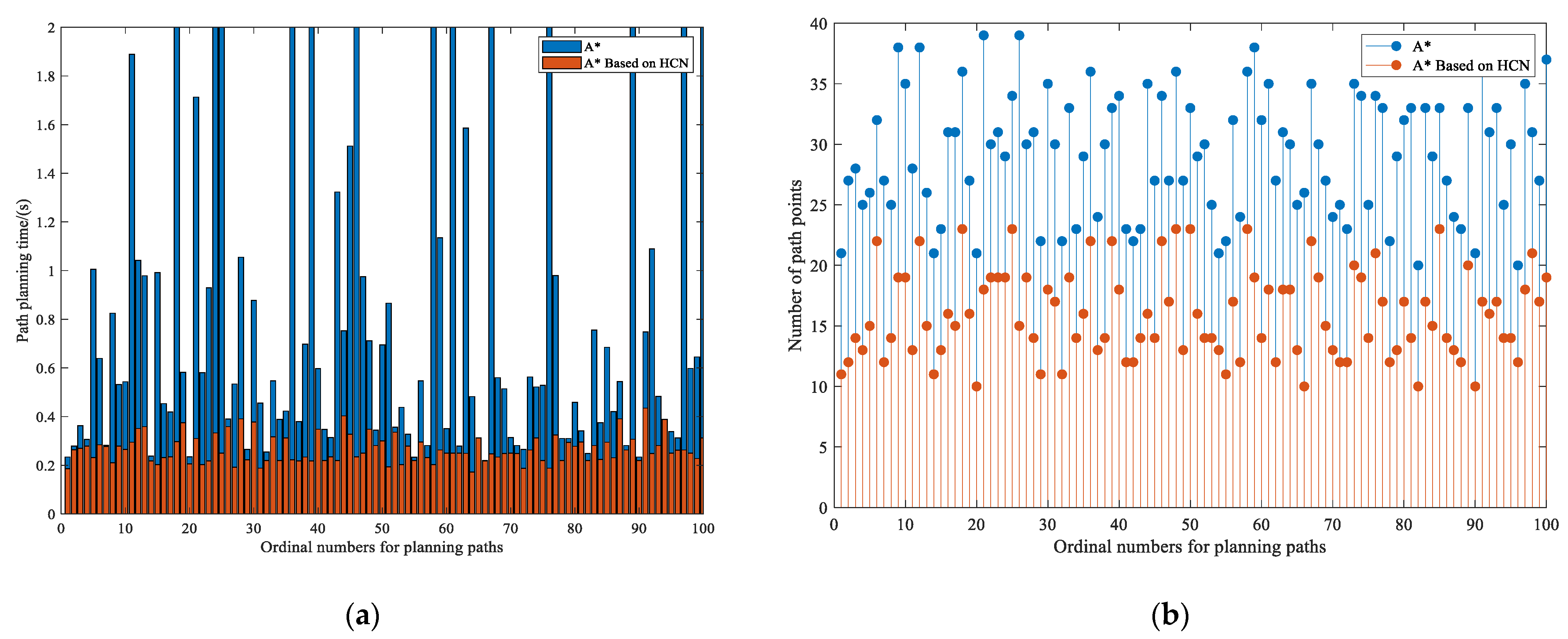
  • The use of HCN in collision-free path planning of manipulators can reduce the average number of path points of the path by 45.5% and reduce the average time of path planning by 48.4%, which greatly improves the efficiency of path planning under resource constraints.
The proposed network and strategy only carry out simulation verification with 3-DOF manipulator and A* algorithm, but its concept can be extended to other manipulators and path planning algorithms. Furthermore, by designing dynamic adjustment strategies, the proposed strategy can be used for dynamic and unknow situation.

Author Contributions

Conceptualization, G.C. and J.F.; methodology, J.F.; software, R.W.; validation, G.C., J.F. and R.W.; formal analysis, J.F.; investigation, C.L. and J.F.; resources, Q.J.; data curation, R.W.; writing—original draft preparation, J.F.; writing—review and editing, G.C. and R.W.; visualization, G.C.; supervision, G.C.; project administration, Q.J.; funding acquisition, G.C. and Q.J. All authors have read and agreed to the published version of the manuscript.

Funding

This research was funded by the National Natural Science Foundation of China, grant number No. 62173044; the National Natural Science Foundation of China, grant number No. 51975059; and the State Administration of Science, Technology and Industry for National Defense, grant number No. HTKJ2019KL502012.

Institutional Review Board Statement

Not applicable.

Informed Consent Statement

Not applicable.

Data Availability Statement

Not applicable.

Conflicts of Interest

The authors declare no conflict of interest. The funders had no role in the design of the study; in the collection, analyses, or interpretation of data; in the writing of the manuscript, or in the decision to publish the results.

References

  1. Bostelman, R.; Hong, T.; Marvel, J. Survey of Research for Performance Measurement of Mobile Manipulators. J. Res. Natl. Inst. Stand. Technol. 2016, 121, 342–366. [Google Scholar] [CrossRef]
  2. Rahmani, B.; Belkheiri, M. Adaptive Neural Network Output Feedback Control for Flexible Multi-Link Robotic Manipulators. Int. J. Control 2019, 92, 2324–2338. [Google Scholar] [CrossRef]
  3. Yang, C.; Li, Q.C.; Chen, Q.H. Multi-objective optimization of parallel manipulators using a game algorithm. Appl. Math. Model. 2019, 74, 217–243. [Google Scholar] [CrossRef]
  4. Farsoni, S.; Ferraguti, F.; Bonfe, M. Safety-oriented robot payload identification using collision-free path planning and decoupling motions. Rob. Comput. Integr. Manuf. 2019, 59, 189–200. [Google Scholar] [CrossRef]
  5. Chaari, I.; Koubaa, A.; Bennaceur, H.; Ammar, A.; Alajlan, M.; Youssef, H. Design and performance analysis of global path planning techniques for autonomous mobile robots in grid environments. Int. J. Adv. Rob. Syst. 2017, 14, 1729881416663663. [Google Scholar] [CrossRef]
  6. Dijkstra, E.W. A note on two problems in connexion with graphs. Numer. Math. 1959, 1, 269–271. [Google Scholar] [CrossRef] [Green Version]
  7. Hart, P.E.; Nilsson, N.J.; Raphael, B. A Formal Basis for the Heuristic Determination of Minimum Cost Paths. IEEE-Trans. Syst. Sci. Cybern. 1968, 4, 100–107. [Google Scholar] [CrossRef]
  8. Liu, C.; Mao, Q.; Chu, X.; Xie, S. An Improved A-Star Algorithm Considering Water Current, Traffic Separation and Berthing for Vessel Path Planning. Appl. Sci. 2019, 9, 1057. [Google Scholar] [CrossRef] [Green Version]
  9. Trovato, K.I.; Dorst, L. Differential A*. IEEE Trans. Knowl. Data Eng. 2002, 14, 1218–1229. [Google Scholar] [CrossRef]
  10. Das, P.K.; Behera, H.S.; Pradhan, S.K.; Tripathy, H.K.; Jena, P.K. A Modified Real Time A* Algorithm and Its Performance Analysis for Improved Path Planning of Mobile Robot. Smart Innov. Syst. Technol. 2015, 32, 221–234. [Google Scholar]
  11. Fu, B.; Chen, L.; Zhou, Y.; Dong, Z.; Pan, H. An improved A* algorithm for the industrial robot path planning with high success rate and short length. Rob. Autom. Syst. 2018, 106, 26–37. [Google Scholar] [CrossRef]
  12. Metea, M.B.; Tsai, J.P. Route planning for intelligent autonomous land vehicles using hierarchical terrain representation. In Proceedings of the 1987 IEEE International Conference on Robotics and Automation, Raleigh, NC, USA, 31 March–3 April 1987; pp. 1947–1952. [Google Scholar]
  13. Qin, L.; Hu, Y.; Yin, Q.J.; Zeng, J. Speed Optimization for Incremental Updating of Grid-Based Distance Maps. Appl. Sci. 2019, 9, 2029. [Google Scholar] [CrossRef] [Green Version]
  14. Duchon, F.; Babinec, A.; Kajan, M.; Beno, P.; Florel, M.; Fico, T.; Jurisica, L. Path Planning with Modified a Star Algorithm for a Mobile Robot. Procedia Eng. 2014, 96, 59–69. [Google Scholar] [CrossRef] [Green Version]
  15. Zuo, L.; Guo, Q.; Xu, X.; Fu, H. A hierarchical path planning approach based on A* and least-squares policy iteration for mobile robots. Neurocomputing 2015, 170, 257–266. [Google Scholar] [CrossRef]
  16. Lozanoperez, T.; Wesley, M.A. An Algorithm for Planning Collison-Free Paths among Polyhedral Obstacles. Commun. ACM 1979, 22, 560–570. [Google Scholar] [CrossRef]
  17. Storer, J.A.; Reif, J.H. Shortest Paths in the Plane with Polygonal Obstacles. J. Assoc. Comput. Mach. 1994, 41, 982–1012. [Google Scholar] [CrossRef]
  18. Lozano-Perez, T. Spatial planning: A configuration space approach. IEEE Trans. Comput. 1983, C-32, 108–120. [Google Scholar] [CrossRef] [Green Version]
  19. LaValle, S.M.; Kuffner, J.J., Jr. Randomized Kinodynamic Planning. Int. J. Rob. Res. 2001, 20, 378–400. [Google Scholar] [CrossRef]
  20. Canny, J.; Donald, B. Simplified Voronoi Diagrams. In Proceedings of the 3rd Annual Symposium on Computational Geometry, Waterloo, ON, Canada, 8–10 June 1987; pp. 219–236. [Google Scholar]
  21. Takahashi, O.; Schilling, R.J. Motion planning in a plane using generalized Voronoi diagrams. IEEE Trans. Rob. Autom. 1989, 5, 143–150. [Google Scholar] [CrossRef]
  22. Kalra, N.; Ferguson, D.; Stentz, A. Incremental reconstruction of generalized Voronoi diagrams on grids. Rob. Autom. Syst. 2009, 57, 123–128. [Google Scholar] [CrossRef] [Green Version]
  23. Uster, H.; Dalal, J. Strategic emergency preparedness network design integrating supply and demand sides in a multi-objective approach. IISE Trans. 2017, 49, 395–413. [Google Scholar] [CrossRef]
  24. Zhou, X.X.; Zhang, H.P.; Ji, G.L.; Tang, G.A. A Method to Mine Movement Patterns between Zones: A Case Study of Subway Commuters in Shanghai. IEEE Access 2019, 7, 67795–67806. [Google Scholar] [CrossRef]
  25. Mostajabdaveh, M.; Gutjahr, W.J.; Sibel Salman, F. Inequity-averse shelter location for disaster preparedness. IISE Trans. 2019, 51, 809–829. [Google Scholar] [CrossRef]
  26. Legowski, A.; Niezabitowski, M. An industrial robot singular trajectories planning based on graphs and neural networks. AIP Conf. Proc. 2016, 1738, 480057. [Google Scholar]
  27. Qureshi, A.H.; Ayaz, Y. Potential functions based sampling heuristic for optimal path planning. Auton. Robot. 2016, 40, 1079–1093. [Google Scholar] [CrossRef] [Green Version]
  28. Gang, L.; Wang, J.F. PRM path planning optimization algorithm research. WSEAS Trans. Syst. Control 2015, 10, 148–153. [Google Scholar]
  29. Bottin, M.; Rosati, G. Trajectory Optimization of a Redundant Serial Robot Using Cartesian via Points and Kinematic Decoupling. Robotics 2019, 8, 101. [Google Scholar] [CrossRef] [Green Version]
  30. Karaman, S.; Frazzoli, E. Sampling-based Algorithms for Optimal Motion Planning. Int. J. Robot. Res. 2011, 30, 846–894. [Google Scholar] [CrossRef]
  31. Kanungo, T.; Mount, D.M.; Netanyahu, N.S.; Piatko, C.D.; Silverman, R.; Wu, A. An efficient k-means clustering algorithm: Analysis and implementation. IEEE Trans. Pattern Anal. Mach. Intell. 2002, 24, 881–892. [Google Scholar] [CrossRef]
  32. Rouane, O.; Belhadef, H.; Bouakkaz, M. Combine clustering and frequent itemsets mining to enhance biomedical text summarization. Expert. Syst. Appl. 2019, 135, 362–373. [Google Scholar] [CrossRef]
  33. Peng, J.H.; Wang, W.; Yu, Y.Q.; Gu, H.L.; Huang, X.H. Clustering Algorithms to Analyze Molecular Dynamics Simulation Trajectories for Complex Chemical and Biological Systems. Chin. J. Chem. Phys. 2018, 31, 404–420. [Google Scholar] [CrossRef]
Figure 1. Diagram of problem transformation. Machines 10 00071 i001 
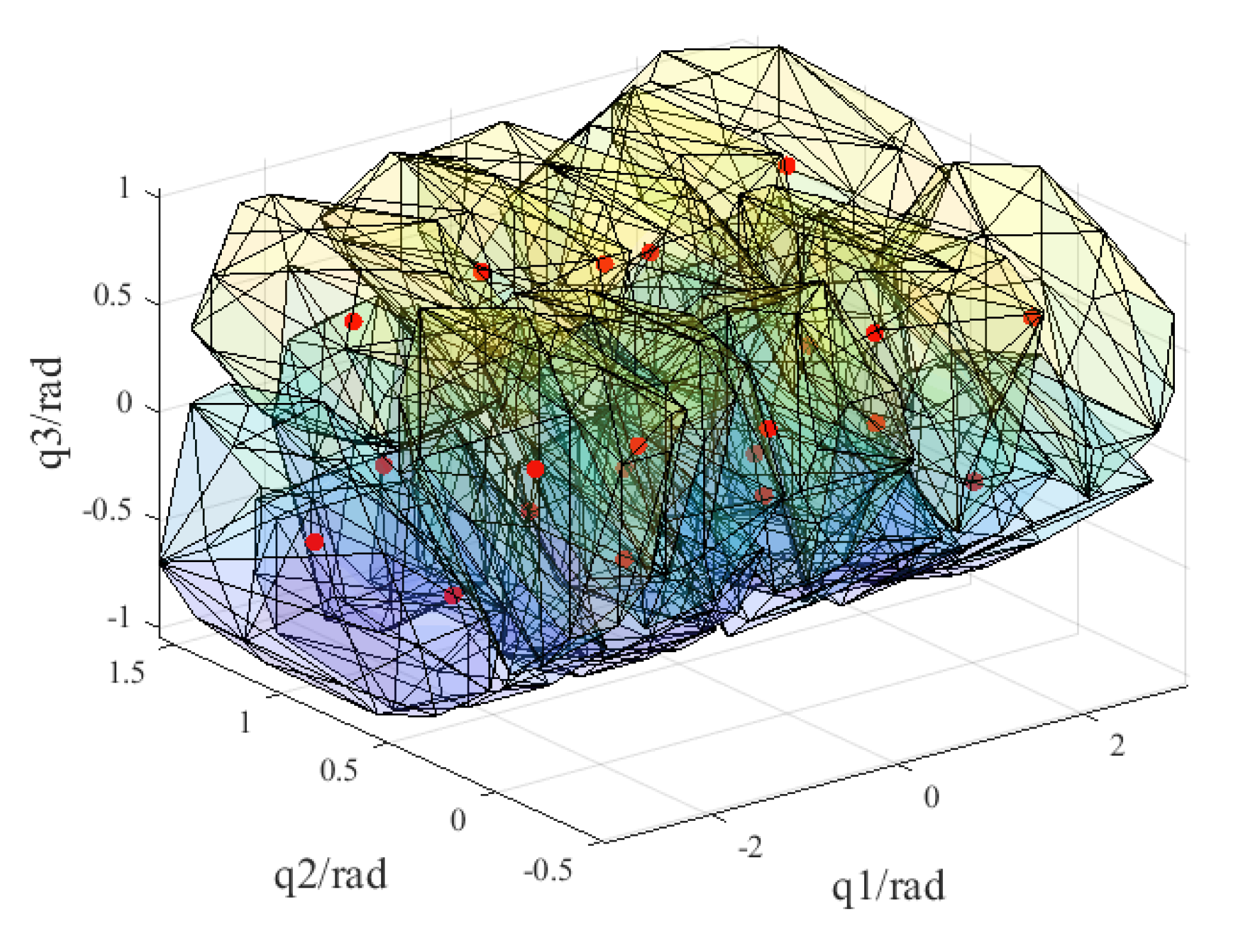
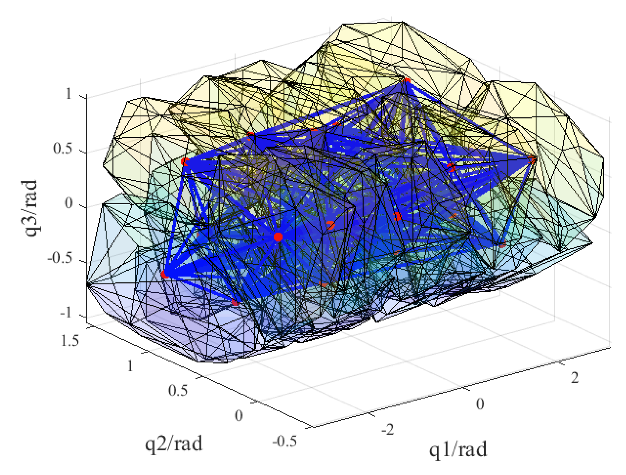
denotes a configuration of the manipulator. The blue line indicates that there are possible collision-free paths between two configurations.
Machines 10 00071 g001
Figure 2. Schematic diagram of the joint space path planning from P initial - to P goal -based network.
Machines 10 00071 g002
Figure 3. Diagram of hub configurations connection.
Machines 10 00071 g003
Figure 4. Process of HCN construction.
Machines 10 00071 g004
Figure 5. The simplified model of the 3-DOF manipulator.
Machines 10 00071 g005
Figure 6. The work space of the manipulator in Cartesian space. (a) 3D view; (b) top view.
Machines 10 00071 g006
Figure 7. Relationship between hub configurations and the functions h 1 ( p ) and h 2 ( p ) .
Machines 10 00071 g007
Figure 8. The result of work space division in joint space.
Machines 10 00071 g008aMachines 10 00071 g008b
Figure 9. The selected hub configurations.
Machines 10 00071 g009
Figure 10. The HCN of the 3-DOF manipulator.
Machines 10 00071 g010
Figure 11. Comparison of collision-free path planning of manipulators using different maps. (a) Planning time; (b) path points.
Machines 10 00071 g011
Table 1. Definitions of some variables.
VariableDefinition
nthe degrees-of-freedom (DOF) of a manipulator
qithe angle of the ith joint, i = 1,2, …, n
P = [ q 1 , , q n ] T n a configuration, i.e., joint angles of the manipulator
M = { P 1 , P 2 , , P m } a set consisting of m configurations
H n a hub configuration
P H = { H 1 , H 2 , , H p } a set consisting of p hub configurations
Ω i = { P 1 , , P N _ g i } a   set   consisting   of   N _ g i configurations, i = 1,2, …, p
w i = [ q w 1 , , q w n ] T n the   center   configuration   in   the   region   Ω i , i = 1,2, …, p
P C = { w 1 , w 2 , , w p } a set consisting of p center configurations
Table 2. DH parameter of the manipulator.
Link iα (°)A (mm)θ (°)d (mm)
10001000
2900−900
3055000
E9000550
Table 3. Obstacle Setting.
ObstacleCenter (mm)Radius (mm)
1[−400; 400; −400]300
Table 4. The comparison between the experiments.
Experiment 1Experiment 2Lower than Experiment 1
Planning time/(s)Max33.9940.4350.992646
Min0.2190.1720.002571
Average2.5856190.265660.484
Path pointsMax39230.615385
Min20100.30303
Average29.1915.930.455
Publisher’s Note: MDPI stays neutral with regard to jurisdictional claims in published maps and institutional affiliations.

