Reinforcement Learning Control of Hydraulic Servo System Based on TD3 Algorithm

Abstract

This paper aims at the characteristics of nonlinear, time-varying and parameter coupling in a hydraulic servo system. An intelligent control method is designed that uses self-learning without a model or prior knowledge, in order to achieve certain control effects. The control quantity can be obtained at the current moment through the continuous iteration of a strategy–value network, and the online self-tuning of parameters can be realized. Taking the hydraulic servo system as the experimental object, a twin delayed deep deterministic (TD3) policy gradient was used to reinforce the learning of the system. Additionally, the parameter setting was compared using a deep deterministic policy gradient (DDPG) and a linear–quadratic–Gaussian (LQG) based on linear quadratic Gaussian objective function. To compile the reinforcement learning algorithm and deploy it to the test platform controller for testing, we used the Speedgoat prototype target machine as the controller to build the fast prototype control test platform. MATLAB/Coder and compute unified device architecture (CUDA) were used to generate an S-function. The results show that, compared with other parameter tuning methods, the proposed algorithm can effectively optimize the controller parameters and improve the dynamic response of the system when tracking signals.

1. Introduction

As a high-precision closed-loop control system, a hydraulic servo system can make the output (displacement, velocity or force) of a system follow the changes of the input quickly and accurately. This offers the unique advantages of fast response speed, large load stiffness and large control power and is widely used in the aerospace, heavy industry, robotics and national defense fields. However, as a high-order nonlinear system, the inherent nonlinearity, time-variability and parameter coupling of a hydraulic servo system pose challenges to the design of control methods [1]. The determination of controller parameters and the deployment of a control strategy are the main difficulties. Thus, the question of how to control a hydraulic servo system with high precision is of great significance to its popularization and application.

The use of reinforcement learning algorithms to solve control problems such as nonlinear engineering problems has been widely studied by many researchers. For instance, Wu, M. et al. [2] used a safe deep reinforcement learning (DRL) control method based on a safe reward shaping method and applied it to the constrained control for an electro-hydraulic servo system (EHSS). Chen, P. et al. [3] proposed a novel control strategy of speed servo systems based on deep reinforcement learning, which can achieve proportional–integral–derivative automatic tuning and effectively overcome the effects of inertia mutation and torque disturbance. Wyrwał, D. et al. [4] proposed a novel control strategy for a hydraulic cylinder based on deep reinforcement learning, which can automatically control the hydraulic system online so that the system can consequently maintain a consistently good control performance. Zhang, T. et al. [5] proposed a strategy based on deep reinforcement learning for the optimization of gain parameters of a cross-coupled controller, allowing the effective convergence of the gain parameters with the optimal intervals. The optimal gain parameters obtained by the proposed strategy can significantly improve the contour control accuracy in biaxial contour tracking tasks. Zamfirache, I.A. et al. [6] proposed a new control approach based on reinforcement learning (RL) that used policy iteration (PI) and a metaheuristic grey wolf optimizer (GWO) algorithm to train neural networks (NNs). In so doing they demonstrated good results for NN training and the solving of complex optimization problems. Shuprajhaa, T. et al. [7] developed a generic-data-driven modified proximal policy optimization (m-PPO) for an adaptive PID controller (RL-PID) based on reinforcement learning for the control of open-loop unstable processes, which eliminated the need for process modeling and pre-requisite knowledge on process dynamics and controller tuning.

Some studies have also integrated multiple comprehensive methods to achieve optimal control. Vaerenbergh, K.V. et al. [8] presented a practical application of a hybrid approach where reinforcement learning is the global layer to tune the controllers of every subsystem for the problem. It was shown that developing a centralized global controller for systems with many subsystems or complex interactions is usually very hard or even unfeasible. Lv, Y. et al. [9] used an RL-based approximate dynamic programming (ADP) structure to learn the optimal tracking control input of a servo mechanism, where unknown system dynamics were approximated with a three-layer NN identifier. Radac, M.B, and Lala, T. [10] proposed a Q-learning-like data-driven model-free (with unknown process dynamics) algorithm. They used neural networks as generic function approximators and validation on an active suspension system and it was shown to be easily amenable to artificial road profile disturbance generation for the optimal and robust control of a data-driven learning solution. Oh, T.H. et al. [11] proposed a DDPG-based deep RL method to simultaneously design and tune several notch filters and used a real industrial servo system with multiple resonances to demonstrate the proposed method effectively. They found the optimal parameters for several notch filters and successfully suppressed multiple resonances to provide the desired performances. Chen, W. et al. [12] proposed a novel adaptive law for the critical network in an RL framework to address the problem of nonlinear system control, which is driven by historical estimation errors but uses an auxiliary matrix instead of a historical data set, thus reducing the computational effort of the controller.

Reinforcement learning mainly learns and optimizes its own behavioral strategies through the idea and mechanism of trial and error. The behavior acts on the environment and obtains a response from the environment. The response is the evaluation index of the behavior. In the process of constantly interacting with the environment, the agent constantly changes their actions according to the rewards they get from the environment. With enough training, the agent can accumulate experience and then interact with the environment in a way that maximizes reward.

Although many studies have been undertaken in the practice of RL design and have laid a great theoretical foundation, there still exist some challenges and shortcomings. For instance, the classic reinforcement learning methods such as Q-learning do not have good generalizability and are usually only useful for specific tasks. Methods of control that have been optimized by neural network algorithms or genetic algorithms are usually effective only for specific cycle periods, lack on-line learning capabilities and have limited generalizability. Additionally, the experimental research on pure hydraulic servo systems has rarely been concerned with RL, and the verification of tests is relatively simple. As a result, most studies fail to set comparison tests or compile reinforcement learning algorithms for testing and verification.

In this study, the application of a reinforcement learning algorithm as the optimal control is presented Ref. [13]. This algorithm learns the optimal control strategy through direct interaction with objects. A deep neural network based on TD3 reinforcement learning training is introduced to realize this complex control [14,15,16]. Firstly, the feasibility and effectiveness of the controller are verified by simulation, and rapid prototype control is then carried out based on a Speedgoat prototype target machine. A GPU coder and LCT packaging tool are then used to deploy the reinforcement learning control program after the reinforcement learning training is completed. Finally, we verify the rationality of the control scheme and the effectiveness of the control algorithm by experiments.

2. Reinforcement Learning

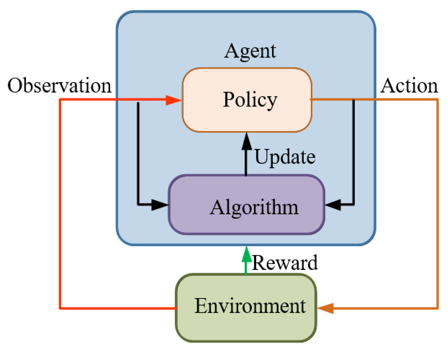
Reinforcement learning [17] is a type of learning method in machine learning. It aims to construct and train agents to complete corresponding tasks in an unknown environment and its basic framework is shown in Figure 1 Since the actions in the learning process can affect the environment and the environment will then affect the subsequent actions, reinforcement learning can be regarded as, in essence, a closed-loop control, and the strategies of the agent allow it to complete the task in an optimal way through iterative updates, which is similar to the controller in the system [18,19].

Interactions between the agent and the environment in a period T are as follows:

(a)

The Agent observes the system state after the previous action A;

(b)

Under the current state of S and strategy P, agent undertakes action A by exploring the noise ϵ;

(c)

The reward value R is obtained under the new environment state S, then the Agent updates the strategy P according to the reward value R;

(d)

Repeat the above steps until the requirements are met.

Among these illustrated above, the reward value R is to evaluate the quality of the actions made by the agent in the environment. Since the reasonable setting of a reward function determines its convergence speed and stability, it is key for the agent to learn strategy effectively.

This paper takes a servo valve controlled asymmetric hydraulic cylinder system as the research object, builds a simulation environment based on a MATLAB/Simulink module, and carries out precise positional control of a hydraulic cylinder through a reinforcement learning algorithm. Additionally, the TD3 reinforcement learning algorithm was designed to interact with the environment so that ultimately the strategy of the control requirements can be satisfied. The servo valve controlled asymmetric hydraulic cylinder system is shown in Figure 2.

3. Design of the Algorithm

3.1. Actor–Critic Algorithm

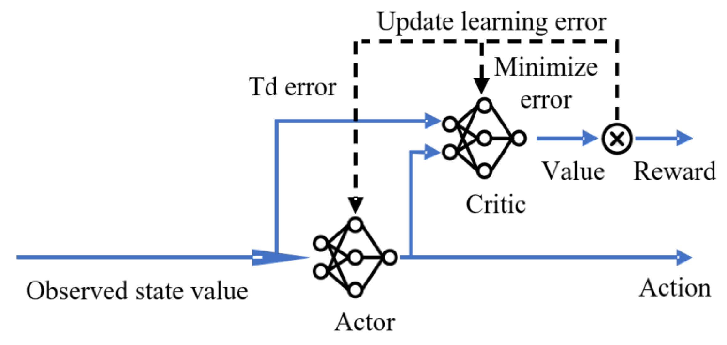
The actor–critic [20] method combines the advantages of two methods: Actor and Critic. The method of Critic can be used to estimate a function of value that can lay a foundation to update the Actor function. As in Figure 3, there are two neural networks, one of these is the Actor network which determines the output in response to the environment, which can be either continuous or discrete. According to the combination of action and state on the output, the Critic network evaluates the value of the action of the Actor network. Meanwhile, the actual reward can be compared with the estimated value of the Critic to get the time difference error (TD-Error), which can judge how to adjust the parameters of the Critic network to obtain a more accurate estimate value. It can also judge the quality of the current action value [21,22], so as to achieve the purpose of updating the Actor parameters. In the process of the constant interaction between the agent and the environment, the weights of the Actor and Critic are updated and a relatively ideal control effect is achieved [23].

3.2. The Algorithm of DDPG and TD3

The depth deterministic policy gradient (DDPG) algorithm is a deep reinforcement learning algorithm based on Actor–Critic architecture for continuous action space [24]. The structure of a DDPG algorithm is shown in Figure 4.

The twin delayed deep deterministic policy gradient (TD3) algorithm (Figure 5) improves the network structure and update mode [25,26,27], which is based on DDPG algorithm.

This uses the Actor–Critic framework and builds six neural networks to build the reinforcement learning body. The reward function is constructed based on the tracking error and error integral of the hydraulic position servo system, and the state set is composed of the output error of the position servo system. The TD3 algorithm has two advantages, which are as follows:

(i) A reduced overestimation of a dual Critic network.

Since noise θ appears in the sample value y, the target value E_θ of Q network in the real case of the learning process is:

$$y=r+\gamma \underset{a^{\prime }}{\max }Q(s^{\prime },a^{\prime })$$

(1)

$$E_{\theta }[\underset{a^{\prime }}{\max }Q(s^{\prime },a^{\prime })+\theta ]\ge \underset{a^{\prime }}{\max }Q(s^{\prime },a^{\prime })$$

(2)

After updating the Q function many times, errors will accumulate, leading to a number of bad states being assigned with higher value, and to a large deviation. A double Q-value network reduces estimation errors because it decouples the action and update operations [28]. The roles of the main and target networks and the update mode are shown in

Table 1. Double Q-value network.

	Main Net	Target Net
Function	Approximation of action value function Q	Providing TD targets
Update	Updating the weights by minimum gradient method	Copy the Main weight

.

Using two independent Critics (sharing experience pool) in the TD3 algorithm, we can take the minimum value between the two Critics to eliminate the phenomenon of overestimation and to update the target value. However, although this may lead to an underestimated value for the strategy, this is preferable to overestimating it, as cumulative overestimation will make the strategy ineffective.

(ii) Smooth regularization of the target strategy.

Each step of the TD update produces a small error, which is more noticeable for approximate estimates. After many updates, a large number of errors will accumulate, eventually leading to an inaccurate Q value [29]. When the Actor and Critic are trained simultaneously, there may be a situation where training is unstable or divergent. In this paper, the target network is introduced by the delayed update of the policy. The method includes two aspects. First, a regularization of the parameters (add noise). Secondly, we update the target network every d times after updating Critic. The update objectives of Critic are calculated by the target network to improve the value function convergence, wherein the value function is updated at a higher frequency and the strategy is updated at a lower frequency.

3.3. Flow of Control

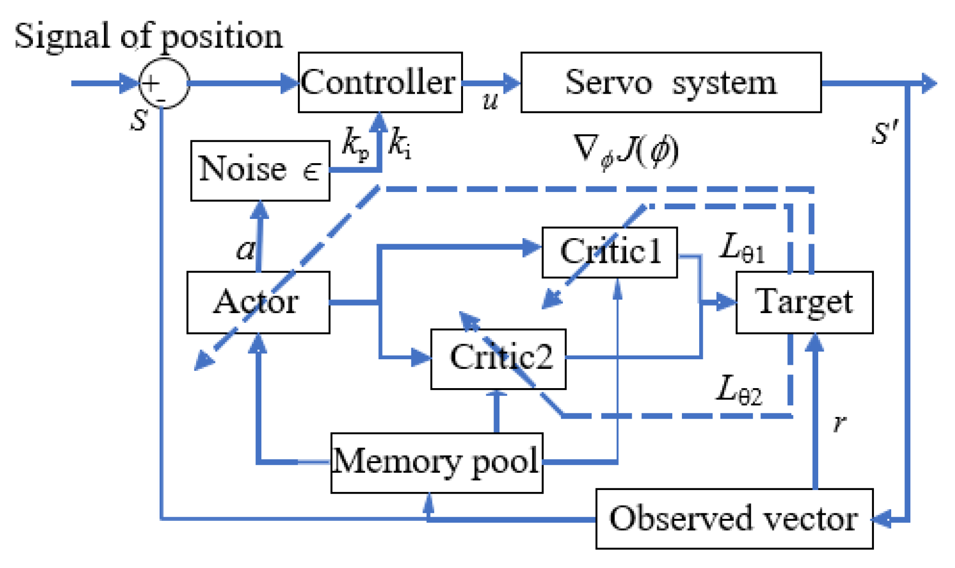
Reinforcement learning in this paper consists of PI parameters K_p and K_i to form an action set, and its learning process is shown in Figure 6 below.

The TD3 servo control algorithm is shown in Figure 7. In the initial target network, we use a DQN mechanism and the initialization playback buffer Β to eliminate the influence of catastrophic neural network forgetting [30,31]. By introducing a random noise with SARSA ideas ϵ (disturbance smooth value function in the action dimensions) to choose a actions and storage transition matrix to B, the memory pool can be formed. The process of updating the weights of Actor and Critic (π_φ, Q_θ1 and Q_θ2) is as follows:

$$\{\begin{array}{l}\tilde{a}\leftarrow {\pi }_{{\varphi }^{\prime }}(s^{\prime })+ϵ\hfill \\ \begin{array}{l}y\leftarrow r+\gamma \underset{i=1,2}{\min }{Q}_{{{\theta }^{\prime }}_i}(s^{\prime },\tilde{a})\\ ϵ~\mathrm{clip}(\eta (0,\tilde{\sigma }),-c,c)\end{array}\hfill \end{array}$$

(3)

Updating the Critic network with minimized loss function:

$$L_{{\theta }_i}=\underset{{\theta }_i}{\min }\frac{1}{N}{(y-Q_{{\theta }_i}(s,a))}^2$$

(4)

Updating Actor networks using policy gradients:

$${\nabla }_{\varphi }J(\varphi )\approx \frac{1}{N}{\displaystyle \sum _i{\nabla }_a{Q}_{{\theta }_1}(s,a){|}_{a={\pi }_{\varphi }(s)}}{\nabla }_{\theta }{\pi }_{\varphi }(s)$$

(5)

Reducing the cumulative error by updating the target network smoothly:

$$\{\begin{array}{c}{{\theta }^{\prime }}_i\leftarrow \tau {\theta }_i+(1-\tau ){{\theta }^{\prime }}_i\hfill \\ {\varphi }^{\prime }\leftarrow \tau \varphi +(1-\tau ){\varphi }^{\prime }\hfill \end{array}$$

(6)

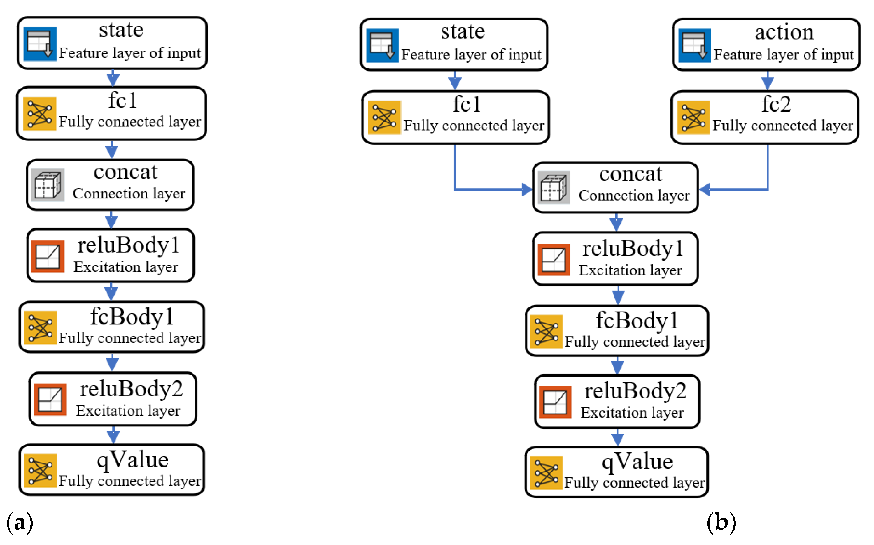
A neural network should be established before creating an Actor network, including an observation input and action output [32]. As a network, a PI controller can set error and error integral observation vectors on the fully connected layer.

$$u=K_{p}e(t)+K_i{\displaystyle {\int }_0^{t}e(t)dt}$$

(7)

$$w=[K_p,K_i]$$

(8)

Here, u is the output of the Actor network and w is the weight of the Actor network.

Since the gradient descent optimization may turn the weight negative, function Y should be executed to ensure that the weights are positive before setting the fully connected PI layer.

$$Y=\mathrm{abs}(w)*[e(t),{\displaystyle {\int }_0^{t}e(t)dt]}$$

(9)

$$J=\underset{T\to \infty }{\lim }E(\frac{1}{T}{\displaystyle {\int }_0^T[A{(ref-y(t))}^2+B{u}^2(t)}]dt)$$

(10)

White noise (E[n²(t)] = 1) is added to the model to simulate signal acquisition and external interference, so as to minimize the output control signal while ensuring minimal errors under the objective function standard.

4. The Establishment of the Environment

4.1. The Establishment of the Network

The reinforcement learning (RL) agent is used to replace the PI controller to keep the network structure of the two Critics in the same state (Figure 8), we then set the number of network neurons (

Table 2. Number of network neurons.

The Name of Layer	Critic Network	Actor Network
Layer of state	3 × 2	3 × 2
Layer of action	4 × 1	-
Fully connected layer 1	50 × 1	50 × 1
Fully connected layer 2	50 × 1	-
Connection layer	32 × 1	32 × 1
Layer of activation 1	25 × 1	25 × 1
Fully connected layer 3	50 × 1	50 × 1
Layer of activation 2	25 × 1	25 × 1
Fully connected layer 4	4 ×1	4 × 1

).

4.2. Establishment of the Environment

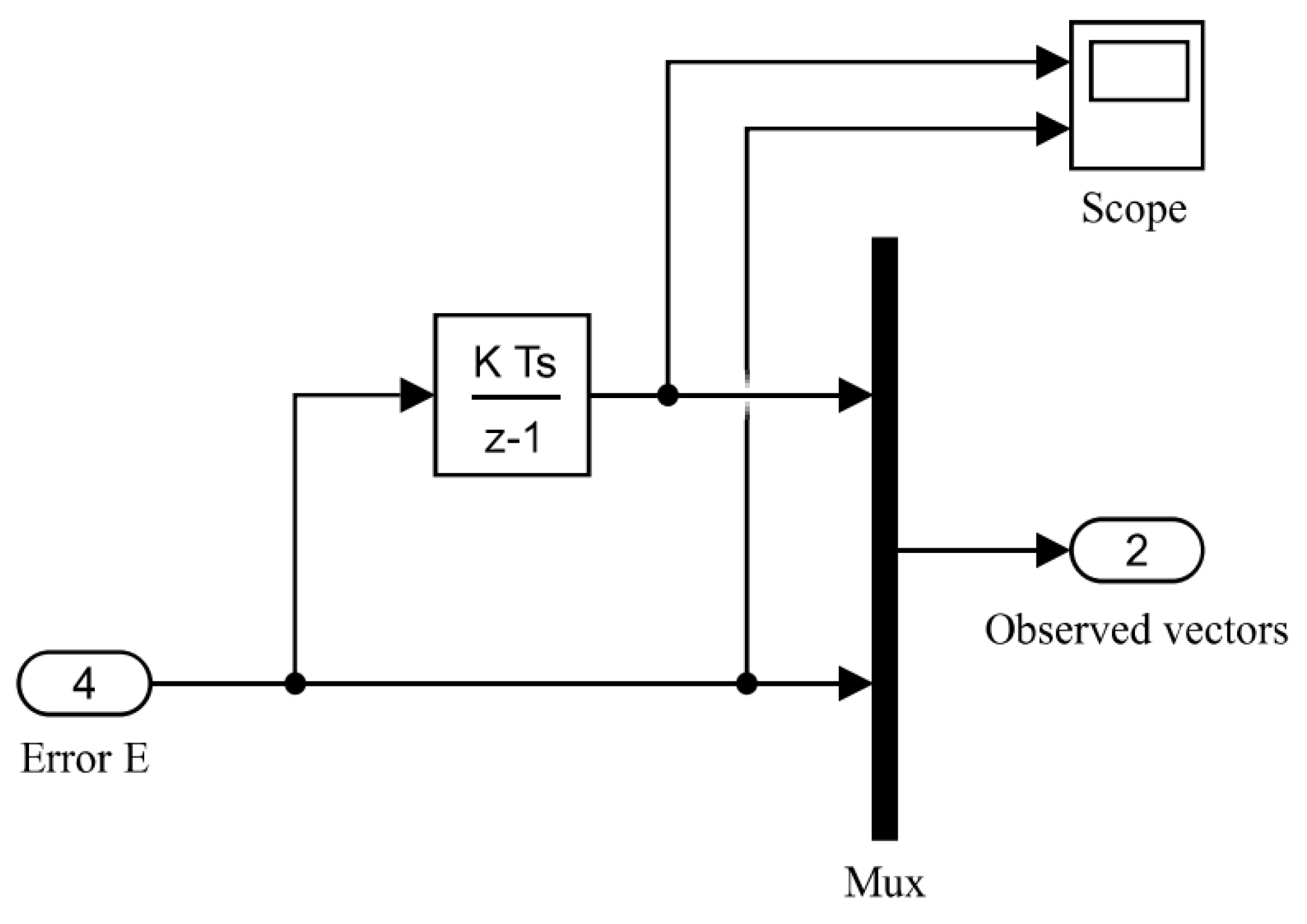
The environment receives operations from agents in reinforcement learning scenarios, outputs observations generated by the dynamic behavior of the environment model and generates rewards to measure the contribution of actions to the completion of tasks [33]. The observer structure is shown in Figure 9.

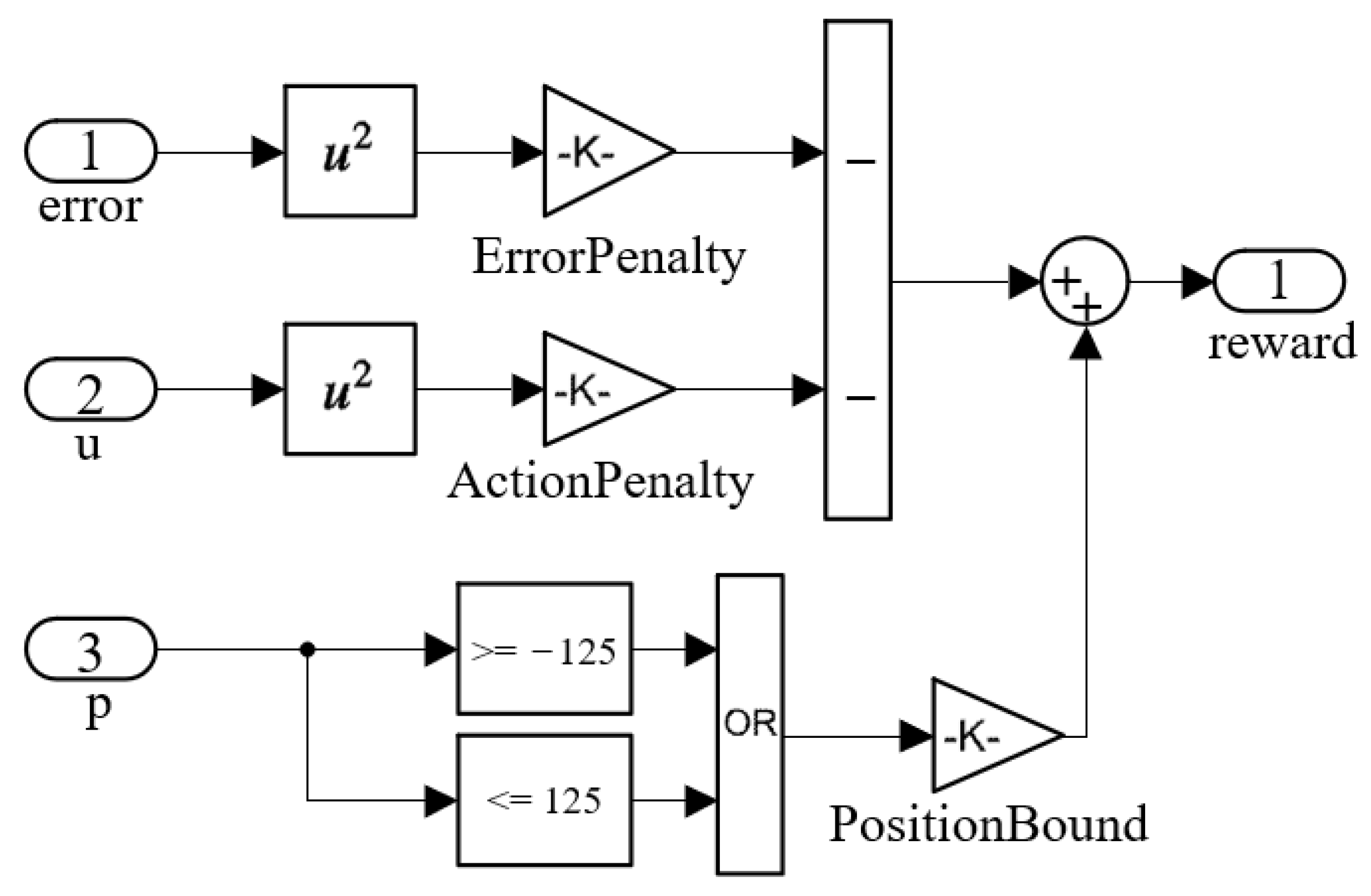
Mixed rewards are used for rewarding signals, which include continuous rewards and discrete rewards. Here, the discrete reward signals keep the system away from the bad state, while continuous reward signals improve the convergence by providing smooth rewards near the target state [34]. The following hybrid reward function R is designed for position control of the hydraulic servo system:

$$\{\begin{array}{c}{r}_1=-{10}^a{e}_{\mathrm{t}}^2-u_{\mathrm{t}}^2\hfill \\ r_2=-{10}^a(p\le -125||p\ge 125)\hfill \\ R=r_1+r_2\hfill \end{array}$$

(11)

The larger a is, the better the network exploration is, but the longer the learning time and the higher the learning cost. When comprehensively considering the parameter a ∈ (1,4), as the displacement is outside the range of activity, there will be a large reward and punishment (P ∈ (125125)). The program block diagram of the above Equation (11) is shown in Figure 10, and the Simulink reinforcement learning training program is shown in Figure 11 below.

4.3. Setting the Hyperparameter

Variables and expressions were used in MATLAB to parameterize the hydraulic model, and the control system of the hydraulic system was designed in Simulink. The super parameters can be set after setting up the environment (

Table 3. Hyperparameter settings.

Hyperparameter	Symbol	Value
Random seed	αr	1
Maximal set	M	2000
Maximum substep size per episode	T	100
Time of sampling	TS	0.01
Time of simulation	Tf	3
Playback buffer	Β	106
Quantity of batch	N	250
Threshold of gradient	ε	1
Learning rate of Actor network	ra	0.0003
Learning rate of Critic network	rc	0.0002
noise of exploration	e	0.1
Delayed updating	D	2
Factor of discount	γ	0.99
Rate of soft renewal	τ	0.01

).

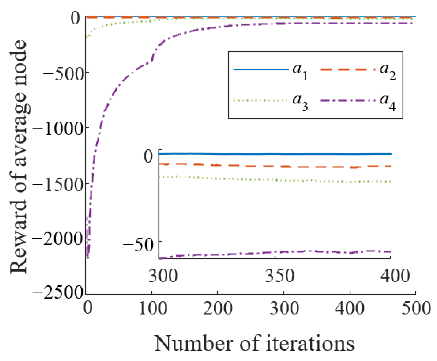
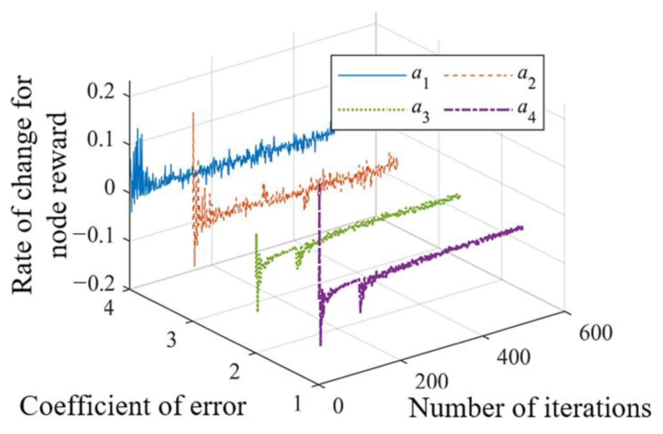
Since training is the foundation of reinforcement learning, the coefficient of the reward function needs to be set several times in normal circumstances, so as to let the agent obtain a better training effect. By setting the error coefficient appropriately, the rates of change for the node reward and average node reward obtained by the agent in training can be shown in Figure 12 and Figure 13 below, where the value of a is set to 1, 2, 3, and 4.

Figure 12 shows the average compensation of agents in training within 500 nodes. The node reward is the actual value of each training round (which fluctuates greatly), while the average reward is the smoothed effect of the actual training (the mean of node training), which eventually increases and becomes stable.

It can be seen from Figure 12 that the smaller the error coefficient is, the greater the final node reward will be, but this does not mean that the smaller the error coefficient is, the better. As can be seen from Figure 13, when the coefficient is 1 or 2, the growth rate of the point reward changes frequently, which means that it is still fluctuating in a small range at 500 steps; however, when the coefficient is 3 or 4, it changes dramatically at the beginning and becomes stable at about 100 steps, while the rate of change in the later period is basically 0. This proves that the first two groups have a higher final reward, though the training was not completed and so the average reward fluctuated wildly. The latter two groups completed the training and, although a higher coefficient of error was set, it ultimately converged to results that are similar to those of the first two groups.

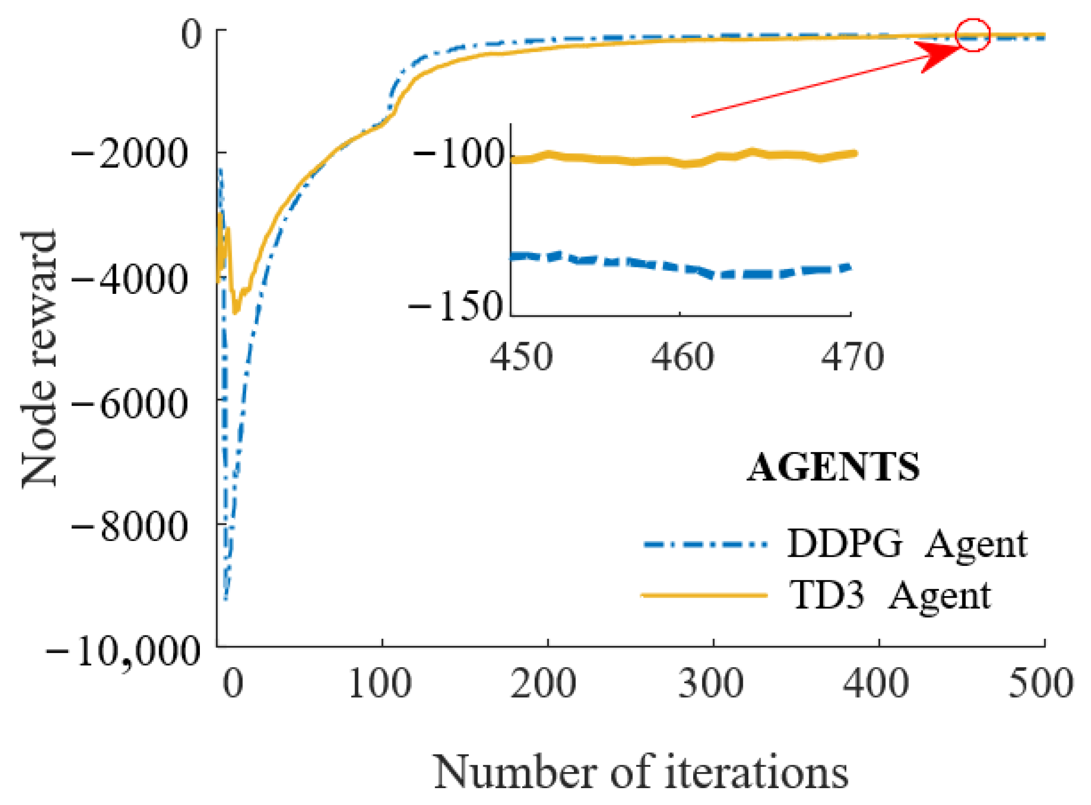
The same reward function was set to compare the training effect of the DDPG and TD3 algorithms. As can be seen from the comparison graph of reinforcement learning curves, DDPG agents learn faster (about 400 sets) and reach the local minimum at the beginning. Compared with DDPG, TD3 has a slower start but a small bottom, and will end up with a higher reward as it avoids the overestimation of the value of Q. Compared with DDPG, TD3 has a steadily improved learning curve, indicating it has improved its stability and the curve graph comparison of learning is shown in Figure 14.

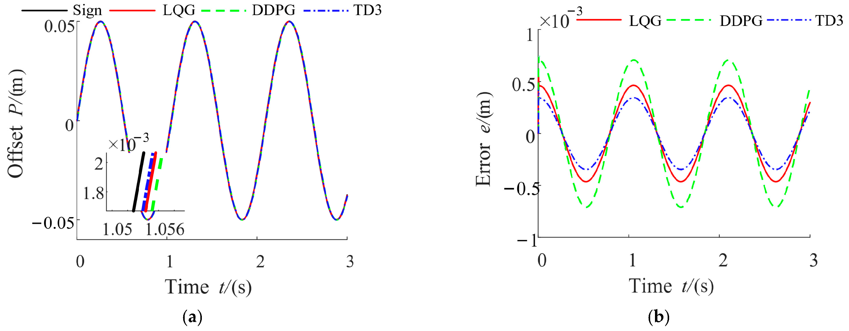
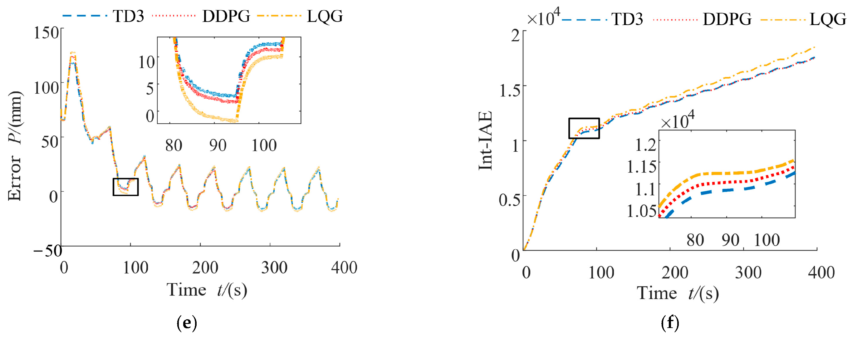
The above reinforcement learning parameter optimization method was compared with the optimal controller (LQG) by simulation experiments, in order to test the actual control performance of the obtained parameters. Under the same input conditions, the response performance of controller parameters obtained by different methods was compared at the same time (the comparison data are shown in Figure 15). Figure 15a,d are sinusoidal signals and trapezoidal signals. It can be seen from the comparison data that TD3 has a better effect than DDPG and LQG as PID controls the errors of the TD3 algorithm. The comparison curves shown in Figure 15b,e are smaller than those of the other two algorithms. Figure 15c,f show the absolute error integral (Int-IAE) curves under the two respective signals. The error cumulative integral (Int-IAE) is taken as the evaluation index to compare the fixed-parameter PID control performance of the control strategy based on reinforcement learning with that of the servo system structure under different signal types and signal amplitude values and shows that, as the cumulative error integral gets smaller, the accuracy increases.

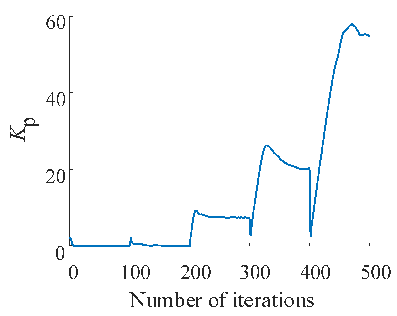
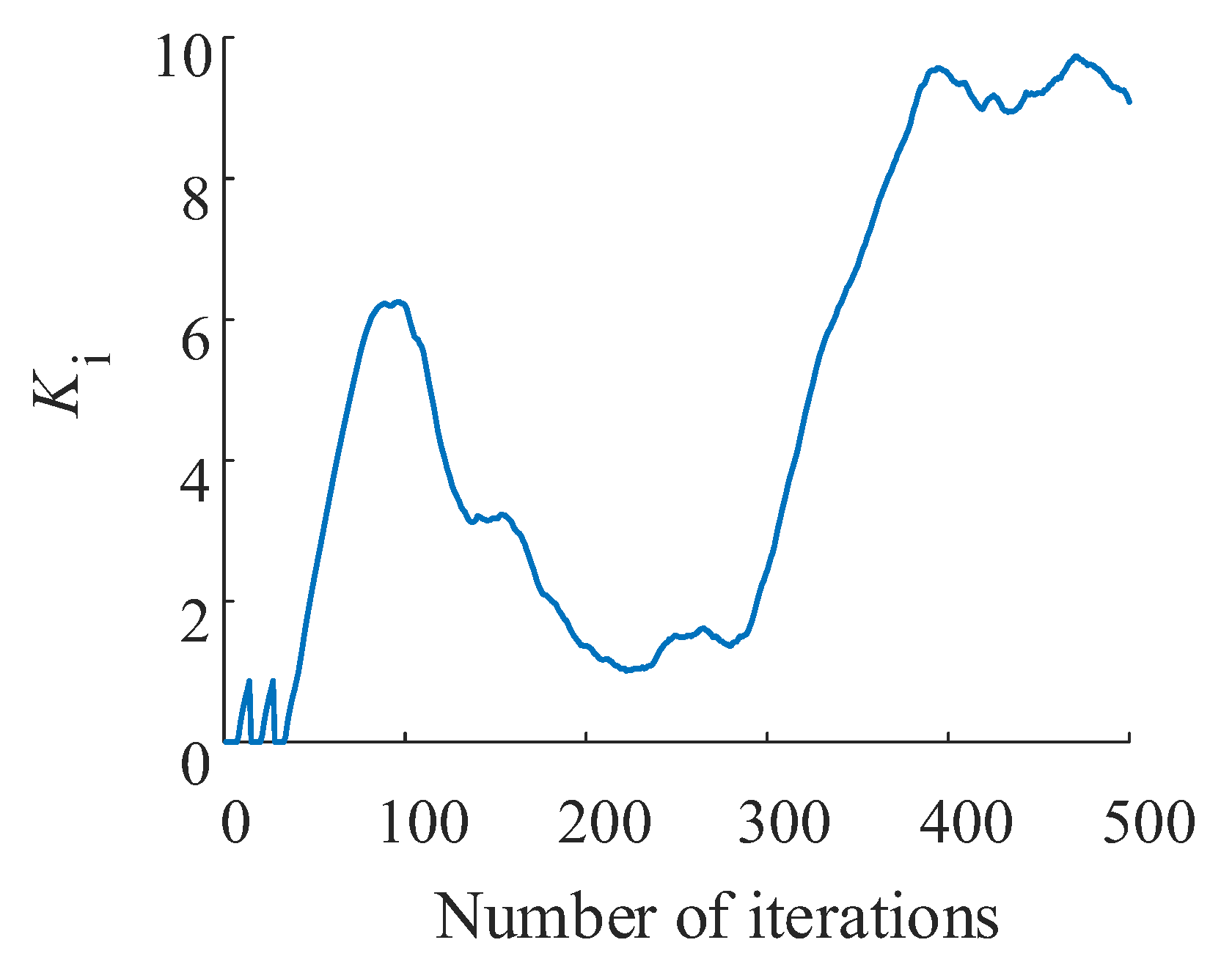
The change of the PI layer parameters after TD3 training is shown in Figure 16 and Figure 17. In the case of the sine and trapezoidal signals, the error and error cumulative integral of the TD3 algorithm are smaller than those of the other two algorithms. It can be seen from

Table 4. System response under step signal.

Strategy	Kp	Ki	Time of Rise (s)	Time of Stability (s)	Overshoot (%)	Phase Margin
LQG	50.52	12.56	0.057	0.102	31	87.45
DDPG	43.41	8.99	0.067	0.114	32	87.85
TD3	54.81	9.11	0.052	0.056	7	87.62

that, compared with DDPG, the overshoot of the TD3 step signal is reduced by 24%, and the stabilization time reaches 0.056 s, which is half as long as that of the LQG, and the overshoot time reaches 7%. The TD3-based reinforcement learning control has relatively simple control tasks with a few adjustable parameters, allowing it to obtain better results. Therefore, the correctness of the agent model and the effectiveness of training can be verified by the above results in this study.

5. Rapid Prototype Control Experiment

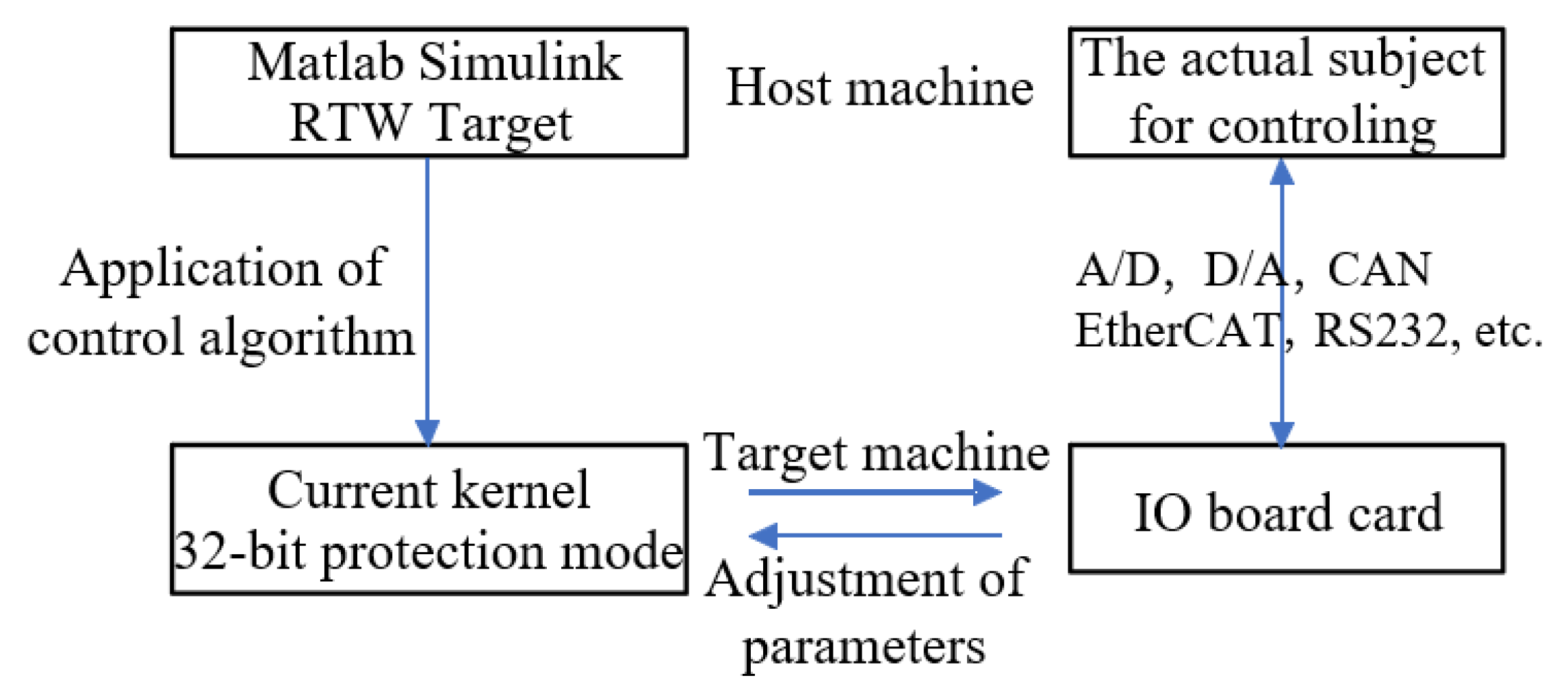
The fast prototype control (Figure 18) is a real-time system that can be created on the desktop, or in a laboratory or field environment. It can also test the automation system and verify its control algorithm, which greatly reduces the development and testing cycle [35].

A better reward function was designed and a greater control strategy was obtained in the simulation environment, both of which are based on the TD3 reinforcement learning environment described above.However, the work needs to be verified by experiment to prove the rationality of the previous work in this paper. The Speedgoat target machine based on a MATLAB kernel can be used for rapid prototype control and to verify the correctness of the simulation results and control strategy.

5.1. Test Equipment

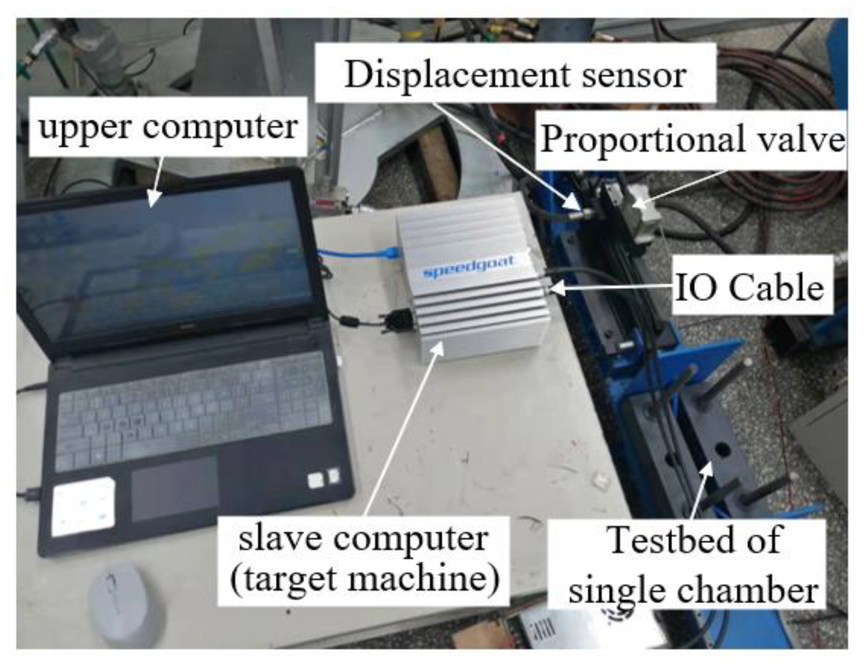
The Speedgoat real-time target machine (Figure 19) in the experiment was used as the controller of the hydraulic servo system, and a rapid prototyping (RP) technology was used to deploy the pure software algorithm to the hardware for implementation, so that it could be tested in a real environment [36,37]. The board configuration of Speedgoat and the mainframe’s technical specifications of Baseline-S are shown in

Table 5. Board configuration of Speedgoat.

Type	Name	Number of Interfaces
Master computer for controlling	Baseline-S Bus	Interfaces of ethernet and video
Input of simulation	IO191 Board card	Single-ended AI of No.24
Output of simulation	IO191 Board card	AO of No.12
CAN Bus	IO691 Board card	No.2
Input of digitization	IO191 Board card	DI of No.24
Output of digitization	IO191 Board card	DO of No.24

and

Table 6. Mainframe’s technical specifications of Baseline-S.

Type	Technical Specifications
CPU	Intel Celeron 2 GHz 4 cores
Current operating system	Simulink Real-Time
memory space	4GB RAM & 32GB SSD
USB interface	1 × USB 3.0 & 2 × USB 2.0
Computer Interface	1 × ethernet interface
serial interface	2 × RS232(Support 120 kb/s)
power supply	9-36V
Protocol Support	TCP/IP, EtherCAT, XCP Master,

respectively.

5.2. Using Reinforcement Learning for Control

To use reinforcement learning-based control, third-party software is required: a CUDA supported NVIDIA GPU; NVIDIA CUDA package and drivers; NVIDIA cuDNN library; Visual Studio compiler; Simulink Real-Time Target Support Package; and other extension packages and environment variables.

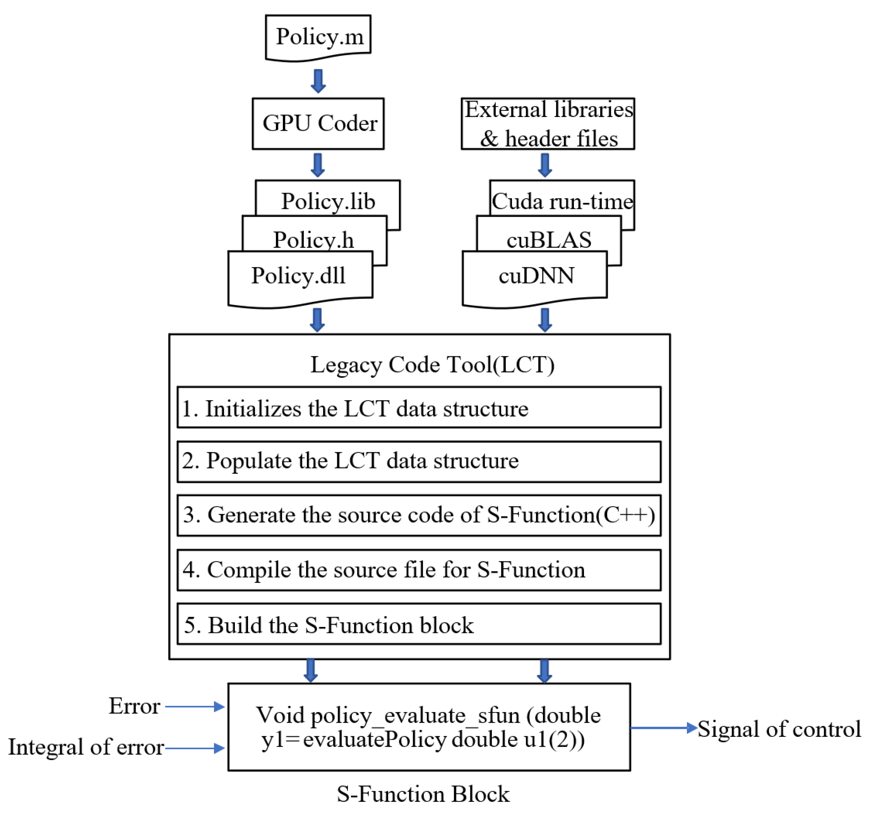
The policy used in this paper uses an extract function to extract the policy part of the agent and generates an “m type” interface function named evaluatePolicy, which is passed to the GPU coder for code generation which generates a series of class dynamic link library codes, whose type is shown in

Table 7. Type of generated code.

Types of Configuring Object	Generated Code
‘Mex’	MEX function
‘Lib’	Static library
‘Dll’	Dynamic library
‘Exe’	Executable file

below.

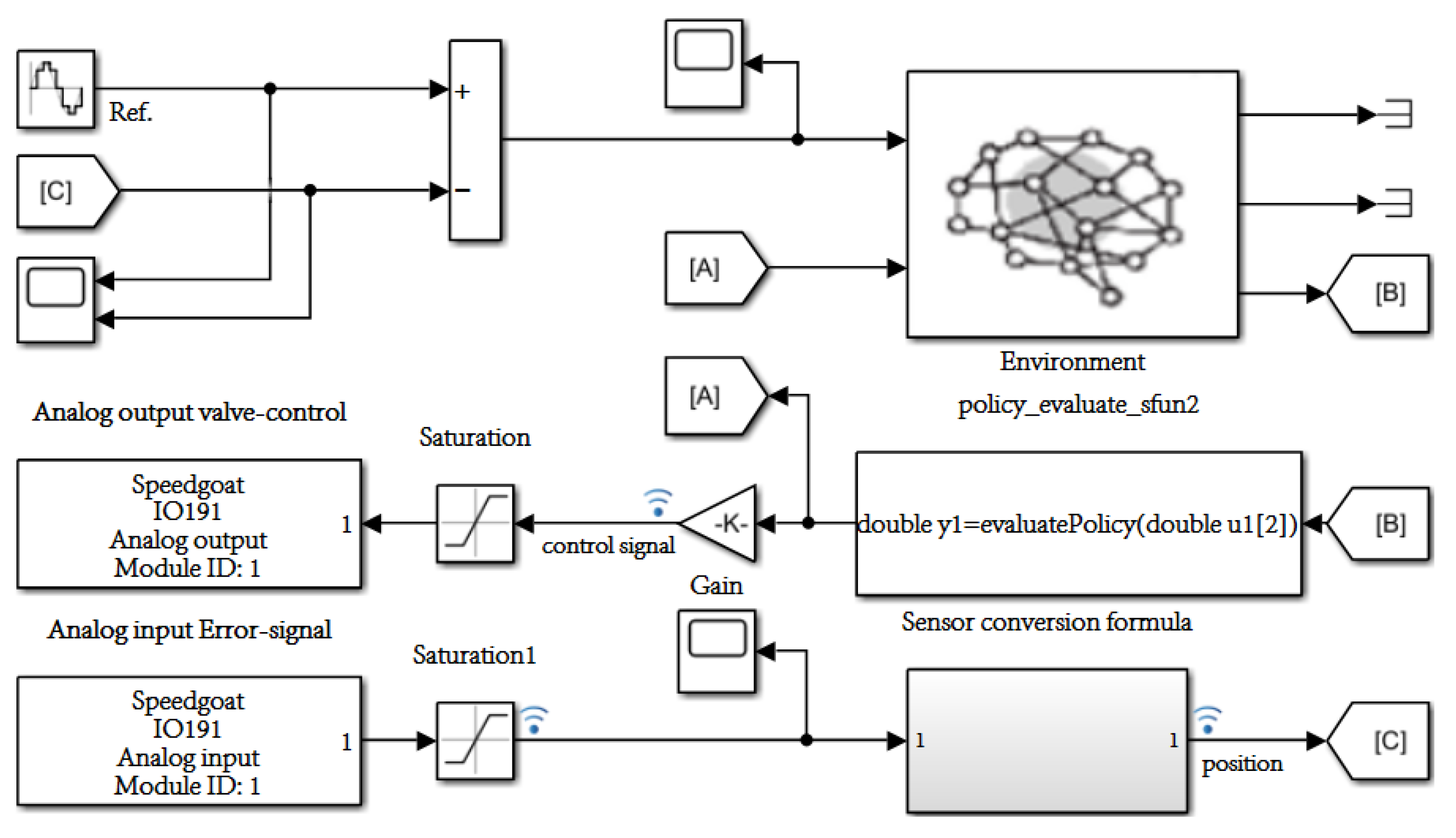
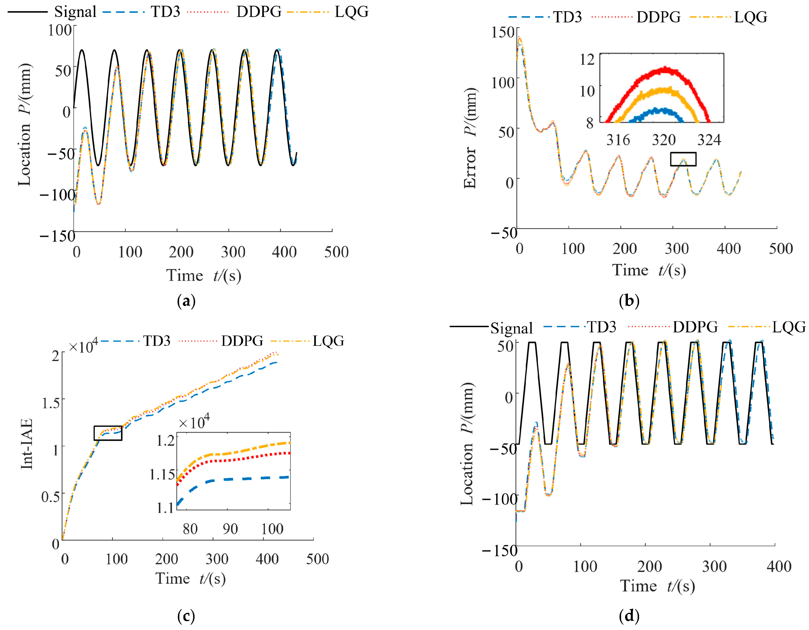
For the hydraulic servo system studied in this paper, a legacy code tool (LCT) was used to encapsulate the dynamic library code into an S-function module, where Figure 20 shows the flow chart of the reinforcement learning control strategy code generation. Figure 21 shows the actual control effect of the control program built on Simulink, which demonstrates that the curve of the experimental results corresponds to the curve of the simulation results and confirms the effectiveness of reinforcement learning control in practical engineering applications. Figure 22 shows the comparison diagram of control method effect.

6. Conclusions

(1)

The reinforcement learning control model of the hydraulic servo system was built based on MATLAB/Simulink. The reinforcement learning model was trained by creating an Actor and Critic layer and defining the observation vector and hyperparameter. The DDPG and TD3 algorithms were trained under the same reward function and the simulation experiments were compared with the linear–quadratic–gaussian (LQG) controller.

(2)

The mixed reward function FR was planned according to the training purpose. When the error coefficient a reaches 4, the average node reward reaches −50, and the average node reward change rate ultimately reaches approximately 0. Thus, it can be seen that the system achieves a higher reward value in the iteration and tends to converge.

(3)

Using the Speedgoat as the reinforcement learning controller, MATLAB/Coder and CUDA were used to generate an S-function, and the reinforcement learning algorithm was compiled and deployed to the test-bed controller for testing by building a fast prototype control test bed for a hydraulic servo system, one which was based on reinforcement learning. The trajectory tracking performance of the proposed algorithm is about 30% higher than that of other algorithms, which verifies the rationality of the control scheme and the effectiveness of the control algorithm.

References

1. Liu, Y.; Wang, A.; Wang, Z.; Liu, C. Research on modeling and model-free control of hydraulic servo system. Mach. Des. Manuf. 2019, 5, 10–13. [Google Scholar]
2. Wu, M.; Liu, L.; Yu, Z.; Li, W. Safe reward-based deep reinforcement learning control for an electro-hydraulic servo system. Int. J. Robust Nonlinear Control. 2022, 32, 7646–7662. [Google Scholar] [CrossRef]
3. Chen, P.; He, Z.; Chen, C.; Xu, J. Control Strategy of Speed Servo Systems Based on Deep Reinforcement Learning. Algorithms 2018, 11, 65. [Google Scholar] [CrossRef] [Green Version]
4. Wyrwał, D.; Lindner, T.; Nowak, P.; Białek, M. Control strategy of hydraulic cylinder based on Deep Reinforcement Learning. In Proceedings of the 2020 International Conference Mechatronic Systems and Materials (MSM), Bialystok, Poland, 1–3 July 2020; pp. 1–5. [Google Scholar]
5. Zhang, T.; Wu, C.; He, Y.; Zou, Y.; Liao, C. Gain parameters optimization strategy of cross-coupled controller based on deep reinforcement learning. Eng. Optim. 2021, 54, 727–742. [Google Scholar] [CrossRef]
6. Zamfirache, I.A.; Precup, R.E.; Roman, R.C.; Roman, R.C.; Petriu, E.M. Policy Iteration Reinforcement Learning-based control using a Grey Wolf Optimizer algorithm. Inf. Sci. Int. J. 2022, 585, 162–175. [Google Scholar] [CrossRef]
7. Shuprajhaa, T.; Sujit, S.K.; Srinivasan, K. Reinforcement learning based adaptive PID controller design for control of linear/nonlinear unstable processes. Appl. Soft Comput. 2022, 128, 109450. [Google Scholar] [CrossRef]
8. Vaerenbergh, K.V.; Vrancx, P.; Hauwere, Y.D.; Nowé, A.; Hostens, E.; Lauwerys, C. Tuning hydrostatic two-output drive-train controllers using reinforcement learning. Mechatronics 2014, 24, 975–985. [Google Scholar] [CrossRef]
9. Lv, Y.; Ren, X.; Zeng, T.; Li, L.; Na, J. Neural Network Tracking Control of Unknown Servo System with Approximate Dynamic Programming. In Proceedings of the 38th Chinese Control Conference, Guangzhou, China, 27–30 July 2019. [Google Scholar]
10. Radac, M.B.; Lala, T. Learning nonlinear robust control as a data-driven zero-sum two-player game for an active suspension system-ScienceDirect. IFAC-PapersOnLine 2020, 53, 8057–8062. [Google Scholar] [CrossRef]
11. Oh, T.H.; Han, J.S.; Kim, Y.S.; Yang, D.Y.; Cho, D.D. Deep RL Based Notch Filter Design Method for Complex Industrial Servo Systems. Int. J. Control. Autom. Syst. 2020, 18, 2983–2992. [Google Scholar] [CrossRef]
12. Chen, W.; Hu, J.; Xu, C.; Zhou, H.; Yao, J.; Nie, W. Optimal tracking control of mechatronic servo system using integral reinforcement learning. Int. J. Control. Autom. Syst. 2022, 16, 1–11. [Google Scholar] [CrossRef]
13. Ding, X.F.; Xu, X.L. Nonlinear Optimal Control of Hydraulic Servo System. Chin. Hydraul. Pneum. 2004, 4, 32–35. [Google Scholar]
14. Yuan, X.; Wang, W.; Zhu, X.; Zhang, L. Theoretical Model of Dynamic Bulk Modulus for Aerated Hydraulic Fluid. Chin. J. Mech. 2022, 35, 121. [Google Scholar] [CrossRef]
15. Wiens, T. Engine speed reduction for hydraulic machinery using predictive algorithms. Int. J. Hydromechatronics 2019, 2, 1. [Google Scholar] [CrossRef]
16. Rehab, I.; Tian, X.; Gu, F.; Ball, A.D. The influence of rolling bearing clearances on diagnostic signatures based on a numerical simulation and experimental evaluation. Int. J. Hydromechatronics 2018, 1, 16–46. [Google Scholar] [CrossRef]
17. Liu, Q.; Zhai, J.; Zhang, Z. A review of deep reinforcement learning. Chin. J. Comput. 2018, 41, 1–27. [Google Scholar]
18. Sung, O.; Jin, K. The design of a real-time simulator on the hydraulic servo system. Int. J. Precis. Eng. Manuf. 2003, 4, 9–14. [Google Scholar]
19. Yang, X.; He, H.; Wei, Q.; Luo, B. Reinforcement learning for robust adaptive control of partially unknown nonlinear systems subject to unmatched uncertainties. Inf. Sci. 2018, 463–464, 307–322. [Google Scholar] [CrossRef]
20. Chen, X.; Yang, Y. Adaptive PID control based on Actor-Critic learning. Control. Theory Appl. 2011, 28, 1187–1192. [Google Scholar]
21. Gao, Q.; Zhu, Y.; Liu, J. Dynamics modelling and control of a novel fuel metering valve actuated by two binary-coded digital valve arrays. Machines 2022, 10, 55. [Google Scholar] [CrossRef]
22. Chao, Q.; Xu, Z.; Tao, J.; Liu, C. Capped piston: A promising design to reduce compressibility effects, pressure ripple and cavitation for high-speed and high-pressure axial piston pumps. Alex. Eng. J. 2023, 62, 509–521. [Google Scholar] [CrossRef]
23. Li, J.; Ji, L.; Li, J. Optimal consensus control for unknown second-order multi-agent systems: Using model-free reinforcement learning method-ScienceDirect. Appl. Math. Comput. 2021, 410, 126451. [Google Scholar] [CrossRef]
24. Wei, X.; Zhang, Q.; Jiang, T.; Liang, L. Fuzzy adaptive deep reinforcement learning method for transient optimization of servo systems. J. Xi’an Jiaotong Univ. 2021, 55, 68–77. [Google Scholar]
25. Lee, D.; Lee, S.J.; Yim, S.C. Reinforcement learning-based adaptive PID controller for DPS. Ocean. Eng. 2020, 216, 108053. [Google Scholar] [CrossRef]
26. Zhen, H.; Zhai, H.; Ma, W.; Zhao, L.; Weng, Y.; Xu, Y.; Shi, J.; He, X. Design and tests of reinforcement-learning-based optimal power flow solution generator. Energy Rep. 2022, 8, 43–50. [Google Scholar] [CrossRef]
27. Chu, Z.; Sun, B.; Zhu, D.; Zhang, M.; Luo, C. Motion Control of Unmanned Underwater Vehicles Via Deep Imitation Reinforcement Learning Algorithm. IET Intell. Transp. Systems 2020, 14, 764–774. [Google Scholar] [CrossRef]
28. Zeng, R.; Zhou, J.; Liu, M. Transfer reinforcement learning algorithm for double Q network learning. Appl. Res. Comput. 2021, 38, 1699–1703. [Google Scholar]
29. Liu, P.; Bai, C.; Zhao, Y.; Bai, C.; Zhao, W.; Tang, X. Generating attentive goals for prioritized hindsight reinforcement learning. Knowl.-Based Syst. 2020, 203, 106–140. [Google Scholar] [CrossRef]
30. Yang, Y.; Li, J.; Peng, L. Multi-robot path planning based on a deep reinforcement learning DQN algorithm. CAAI Trans. Intell. Technol. 2020, 5, 177–183. [Google Scholar] [CrossRef]
31. Chen, J.; Yang, Z.; Liu, Q.; Wu, H.; Xu, Y.; Fu, Q. Heuristic Sarsa algorithm based on value function transfer. J. Commun. 2018, 39, 37–47. [Google Scholar]
32. Chen, J.; Zheng, M. A review of robot operating behavior based on deep reinforcement learning. Robot 2022, 44, 236–256. [Google Scholar]
33. Self, R.; Coleman, K.; He, B.; Kamalapurkar, R. Online Observer-Based Inverse Reinforcement Learning. In Proceedings of the 2021 American Control Conference (ACC), New Orleans, LA, USA, 25–28 May 2021; Volume 5, pp. 1959–1964. [Google Scholar]
34. Zhao, Y.; Qin, J.; Yuan, L. Intrinsic rewards that combine novelty and risk assessment. Comput. Eng. Appl. 2022, 1–9. [Google Scholar]
35. Wei, L.; Luo, L.; Wang, Y.; Wang, G. Rapid Control Prototype Design of Electro-hydraulic Position Control Servo System Based on xPC Target. Chin. Hydraul. Pneum. 2018, 7, 24–28. [Google Scholar]
36. Maghareh, A.; Silva, C.E.; Dyke, S.J. Servo-hydraulic actuator in controllable canonical form: Identification and experimental validation. Mech. Syst. Signal Process. 2018, 100, 398–414. [Google Scholar] [CrossRef]
37. Lyu, L.; Chen, Z.; Yao, B. Advanced Valves and Pump Coordinated Hydraulic Control Design to Simultaneously Achieve High Accuracy and High Efficiency. IEEE Trans. Control. Syst. Technol. 2021, 29, 236–248. [Google Scholar] [CrossRef]
Figure 1. The basic framework of reinforcement learning.
Machines 10 01244 g001
Figure 2. The schematic diagram of hydraulic servo system. 1. Asymmetric hydraulic cylinder 2. Sensor 3. Load 4. Servo hydraulic valve 5. Throttle hydraulic valve 6. Relief value 7. Hydraulic oil tank 8. Pump.
Machines 10 01244 g002
Figure 3. The Actor–Critic algorithm.
Machines 10 01244 g003
Figure 4. Structure of a DDPG algorithm.
Machines 10 01244 g004
Figure 5. Structure of TD3 algorithm.
Machines 10 01244 g005
Figure 6. Flow chart of TD3 algorithm.
Machines 10 01244 g006
Figure 7. The servo control algorithm of TD3.
Machines 10 01244 g007
Figure 8. The neural network structure layer defined by TD3. (a) The network layer of the Actor and (b) the network layer of the Critic.
Machines 10 01244 g008
Figure 9. Observed vectors.
Machines 10 01244 g009
Figure 10. Calculation of the reward function.
Machines 10 01244 g010
Figure 11. Block diagram of reinforcement learning.
Machines 10 01244 g011
Figure 12. Reward of average node.
Machines 10 01244 g012
Figure 13. Average rate of change for node reward.
Machines 10 01244 g013
Figure 14. The curve graph comparison of learning.
Machines 10 01244 g014
Figure 15. Comparison diagram of control method effect. (a) Following the sinusoidal signal, (b) subsequent error of the of sinusoidal signal, (c) comparison graph of IAE index, (d) following the trapezoidal signal, (e) error of the subsequent of sinusoidal signal, and (f) comparison graph of IAE index.
Machines 10 01244 g015aMachines 10 01244 g015b
Figure 16. Variation curve of Kp.
Machines 10 01244 g016
Figure 17. Variation curve of Ki.
Machines 10 01244 g017
Figure 18. Fast prototype control.
Machines 10 01244 g018
Figure 19. Fast prototype control of Speedgoat.
Machines 10 01244 g019
Figure 20. Process of code generation.
Machines 10 01244 g020
Figure 21. Rapid prototyping control program of Speedgoat.
Machines 10 01244 g021
Figure 22. Comparison diagram of control method effect. (a) Following the sinusoidal signal, (b) curve of error, (c) absolute error of the of sinusoidal signal, (d) Following the trapezoidal signal, (e) curve of error, and (f) absolute error of the trapezoidal signal.
Machines 10 01244 g022aMachines 10 01244 g022b