Article

Sliding Mode Based Load Frequency Control and Power Smoothing of Power Systems with Wind and BESS Penetration

1
College of Water Conservancy and Hydropower Engineering, Hohai University, Nanjing 210098, China
2
College of Energy and Electric Engineering, Hohai University, Nanjing 211100, China
*
Author to whom correspondence should be addressed.
Machines 2022, 10(12), 1225; https://doi.org/10.3390/machines10121225
Submission received: 2 November 2022 / Revised: 6 December 2022 / Accepted: 13 December 2022 / Published: 15 December 2022
(This article belongs to the Special Issue Optimization and Control of Distributed Energy Systems)

Abstract

:
This study aims to maintain the frequency stability of the power system penetrated by wind power. Hence, a battery energy storage system (BESS) is applied to smooth the wind power output in power systems and to enhance their load frequency control (LFC) capacity. A novel comprehensive control framework is proposed for power systems integrated with wind farms and BESS based on an adaptive fuzzy super-twisting sliding mode control (AF-SSMC) method. Firstly, the sliding functions and control laws of subsystems are designed according to different relative degrees. Then, the super-twisting algorithm is applied to suppress the chattering of the sliding mode control law. Furthermore, an adaptive fuzzy control method is used to adjust the control gains online for better control performance of the controllers. The Lyapunov stability theory is employed to prove the asymptotic stability of the subsystems. The model of an interconnected thermal power system with wind and BESS penetration is also constructed for simulation analyses. The results indicate that the AF-SSMC method effectively reduces the chattering, and the proposed framework stabilizes the frequency of the power system under system uncertainties and external disturbances. Moreover, the wind farm and BESS combined system accurately tracks a reference power to reduce wind power fluctuations.

1. Introduction

With the rapid development of wind energy utilization technologies, an increasing number of wind farms are integrated into electric power systems. Although wind energy is known for its inexhaustible and non-polluting advantages, its intermittent and random characteristics endanger the safety and stability of power systems [1,2]. Moreover, replacing conventional synchronous generators with wind power generators in a power system reduces its inertia response capacity, resulting from the fact that wind power generators are usually decoupled from the power system through power electronic converters [3,4]. Therefore, the power system frequency stability is further affected. All in all, there is an urgent need to address the stability problem caused by the integration of more and more wind farms.
As two effective measures to ensure the stability of power systems under wind power fluctuations, load frequency control (LFC) and wind power smoothing have always attracted a considerable amount of attention. LFC has a pivotal role in maintaining the power system frequency stability, which is realized by mitigating the deviation between the power supply and load demand of the power system [5]. Many studies concerning frequency regulation only through conventional synchronous generators have been reported. For the LFC of power systems with wind integration, methods including adaptive fuzzy control [6,7], PID control [8,9], robust H control [10], event-triggered control [11], and sliding mode control (SMC) [12,13] have been explored. To compensate for the inertia loss of power systems, some studies required wind turbines to provide frequency support through droop control, inertial control, PID control, deloading control, and so on [14,15].
However, there are some limitations to using wind turbines for frequency regulation, including the limited kinetic energy stored in wind turbines [15], secondary frequency drop events during the acceleration process [16], and the increased fatigue load for frequent control actions [8]. Therefore, researchers have shown an increasing interest in utilizing battery energy storage systems (BESS) for frequency regulation due to their fast response, high power and energy density, simple maintenance requirements, and high cycle life [17,18,19]. In terms of wind power smoothing, proper power control of BESS is also regarded as an effective method to reduce power fluctuations, which has drawn great attention [14]. Recently, studies applying BESS to reduce wind power fluctuations are through wind power filtering [17,20], fuzzy control [21], model predictive control (MPC) [22], probabilistic forecasting-based control [23], and so on.
To the best of the authors’ knowledge, there are currently no studies simultaneously considering frequency regulation and wind power smoothing based on the BESS in grid-connected wind farms. The joint control of LFC and wind power smoothing is able to combine the advantages of both. Currently, more and more wind farms are required to be equipped with BESS [24]. By making more efficient use of the BESS, it simultaneously reduces the volatility of grid-connected wind power and provides active power support for reducing grid frequency fluctuations, which helps to better ensure the stability of the power system. This is of significance for the safe and efficient operation of existing power systems.
To simultaneously achieve LFC and wind power smoothing, this study proposes a comprehensive control framework to exploit the BESS equipped in a wind farm effectively. Under this framework, the subsystems in an interconnected thermal power system with wind and BESS penetration (also called a hybrid power system here) cooperate in different ways. Firstly, BESS is applied to regulate system frequency. Secondly, wind power fluctuations are reduced by regulating the BESS power output. To this end, BESS coordinates with the wind farm to track a reference power determined by the transmission system operator (TSO) according to wind power forecasts. To achieve the comprehensive control of a hybrid power system, controllers are, respectively, designed for the subsystems based on sliding mode control (SMC).
SMC is insensitive to external disturbances and system uncertainties, which causes it to receive considerable critical attention [25]. Many studies have employed SMC for the frequency regulation of power systems, and some have also considered the impact of wind power systems being connected to the grid. For the LFC of power systems, Guo proposed a full-order SMC in [12] and then applied an adaptive SMC to deal with external disturbances and parameter variation in [25]. Lv et al. [26] developed SMC controllers to reduce the frequency deviation in multi-area power systems. Narendra et al. [13] employed a centralized SMC for frequency stability enhancement of a microgrid and a selfish herd optimization algorithm was applied to evaluate the control gains. Ansari et al. [5] presented an event-triggered integral SMC scheme with a disturbance observer for the LFC of multi-area power systems. Prasad et al. [27] presented a non-linear SMC for frequency regulation integrative with wind power systems. Deng et al. [28] applied the derivative and integral terminal SMC to stabilize the frequency of wind-integrated power systems. However, BESS was not contained in the previous studies using SMC. In this study, the BESS in the power system is further considered in the sliding mode design, and an equivalent circuit model of BESS is modified for this purpose [29]. Control-oriented BESS models include equivalent circuit models, reduced-order models, and physics-based models, where equivalent circuit models are simpler and easier to couple with other models [30,31]. In this way, BESS is applied to deal with the instability problem caused by wind fluctuations in the power system by participating in LFC and wind power smoothing.
A major problem with SMC is the chattering phenomenon, which may endanger the stability and safety of the control system. Several methods have been proposed to overcome the chattering problem, including the boundary layer technique [32], fractional SMC [33], reaching laws [34,35], and high-order SMC [36]. Among them, high-order SMC is an effective solution to suppress chattering. Compared with other SMC methods, the control variable of high-order SMC is not the control input in the actual system, but its derivative or high-order derivative. In this way, when calculating the actual control variable, the discontinuous control variable becomes continuous through integration, which can greatly weaken the chattering problem. As one of the most widely used high-order SMC methods [37], the super-twisting algorithm is capable of hiding the high-frequency switching part in high-order derivatives of the control variable, suppressing the chattering of the control law and providing a finite-time convergence to the system [38,39]. Thus, the super-twisting algorithm is often applied to different SMC-based control problems to attenuate the chattering phenomena, such as the trajectory tracking of heavy load robots [40], the control problem of the grid-connected power converters [41], and the maximum power tracking of the direct-driven wind power system [42].
Besides, it is difficult to determine the optimal control gains of the controllers by experience and experiment. Adaptive fuzzy algorithms can be used to approximate uncertain parts of the model and cope with changes in controller parameters [43]. Ayas et al. [44] presented an adaptive admittance control method with a fuzzy logic-based gain regulator for the parallel ankle rehabilitation robot. Li et al. [45] applied a fuzzy inference system to regulate the control parameters of an adaptive controller for the energy management of a hybrid vehicle. Fei et al. [38] utilized an adaptive fuzzy algorithm to adjust the controller parameters online for the micro-gyroscope.
To solve the power control problems of the hybrid power system in this study, sliding surfaces and control laws are firstly designed for the subsystems according to different relative degrees. Then, we apply the super-twisting algorithm to improve the performance of sliding mode controllers. Moreover, an adaptive fuzzy control method is employed, which approaches and adjusts control gains online for better control performance. In summary, an adaptive fuzzy super-twisting sliding mode control (AF-SSMC) method is provided for the control design of the subsystems. The major contributions of this study are as below:
(1)
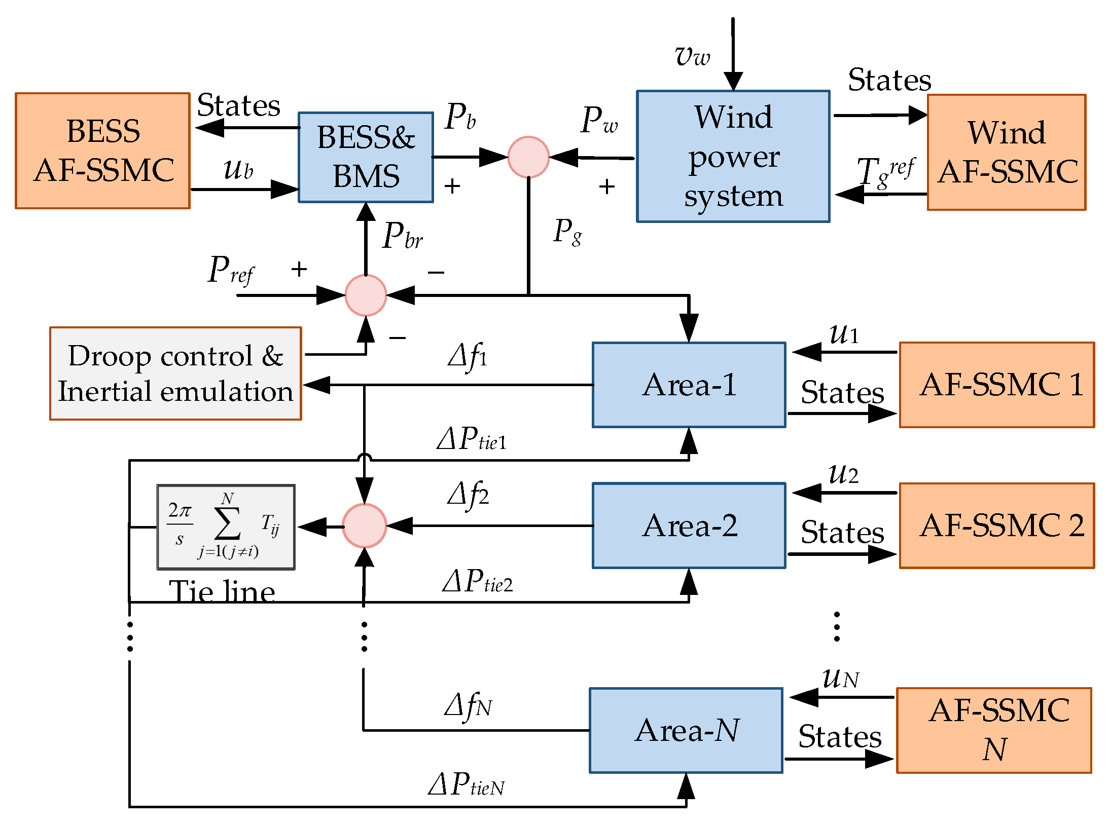
A comprehensive control framework is proposed for interconnected thermal power systems with wind and BESS penetration to maintain frequency stability. In this framework, the BESS is utilized to provide frequency support for the thermal power system. Simultaneously, it reduces the power disturbance from the wind farm to the power system through wind power smoothing;
(2)
AF-SSMC controllers are designed for the subsystems of a hybrid power system to realize precise control. Firstly, sliding functions and control laws are designed for the subsystems according to their relative degrees. Then, the super-twisting algorithm and the adaptive fuzzy control method are employed to suppress chattering and to adjust the control gains online, respectively;
(3)
The model of an interconnected two-area thermal power system with wind and BESS penetration is constructed for simulation analyses. The results indicate that the proposed control framework is effective in frequency regulation and wind power smoothing.
The remaining part of this paper proceeds as follows: The compositions and control problems of the hybrid power system are introduced in Section 2. Then, controllers are designed for the subsystems in Section 3. Section 4 analyzes the control performance of the proposed framework by numerical simulations. Finally, this study is concluded in Section 5.

2. System Configuration
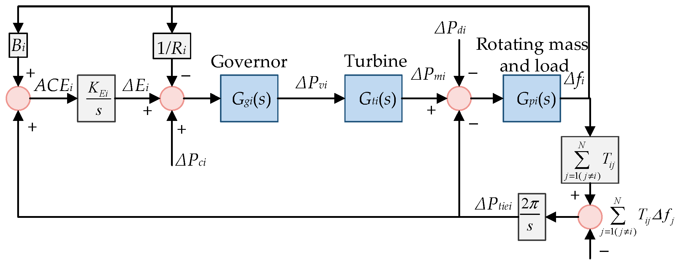
As shown in Figure 1, hybrid power systems often consist of multiple control areas interconnected with tie lines [26]. This study explores the LFC and wind power smoothing of the hybrid power system with wind and BESS penetration. The BESS is integrated into the wind farm first. Then, the combined system, consisting of the wind farm and BESS, is connected to the power system. In a multi-area power system, all areas could be integrated with combined systems. Without loss of generality, only area-1 is deployed with a combined system in Figure 1 for simplification. Pg is the power output of the combined system. To reduce the adverse effects of wind power fluctuations on the stability of the power system, the wind farm should track the reference power Pref provided by the TSO. In the case of accurately tracking the reference power, Pg = Pref should be satisfied. Meanwhile, the BESS improves the frequency response of the power system through droop control and inertial emulation.
The subsystems of a hybrid power system, including the thermal power system, the wind farm, and the BESS, are presented in this section. The wind farm integrated into the power system is represented by a wind power system. The BESS improves the frequency response of the power system and coordinates with the wind farm to track the reference power from the TSO.

2.1. Power System

Figure 2 shows the linearized model of the ith control area in an N-area power system. In a control area, all thermal power turbines are equivalently simplified to a single turbine. The main elements of the model, including the rotating mass and load, a governor, and a turbine, are described as follows [26]:
G p i ( s ) = K p i T p i s + 1
G g i ( s ) = 1 T g i s + 1
G t i ( s ) = 1 T t i s + 1
where Tpi, Tgi, and Tti are, respectively, the electric system time constant, governor time constant, and turbine time constant; Kpi is the power system gain (Hz/MW).
The ith control area is described by the following equations [27]:
Δ f ˙ i ( t ) = 1 T p i Δ f i ( t ) + K p i T p i Δ P m i ( t ) K p i T p i Δ P t i e i ( t ) K p i T p i Δ P d i ( t )
Δ P ˙ m i ( t ) = 1 T t i Δ P m i ( t ) + 1 T t i Δ P v i ( t )
Δ E ˙ i ( t ) = K E i B i Δ f i ( t ) + K E i Δ P t i e i ( t )
Δ P ˙ t i e i ( t ) = 2 π j = 1 ( j i ) N T i j ( Δ f i ( t ) Δ f j ( t ) )
Δ P ˙ v i ( t ) = 1 R i T g i Δ f i ( t ) 1 T g i Δ P v i ( t ) + 1 T g i Δ E i ( t ) + 1 T g i Δ P c i ( t )
where ∆fi(t), ∆Pmi(t), ∆Ei(t), ∆Ptiei(t), and ∆Pvi(t) are selected as system states, they are the deviations in frequency (Hz), generator output (MW), integral control (MW), tie-line power flow (MW) and governor valve position (MW), respectively; the load disturbance ∆Pdi(t) (MW) is an external disturbance acting on the power system; ∆Pci(t) is the control signal to the governor; Bi, KEi, Ri, and Tij are, respectively, the frequency bias factor (Hz/MW), the integral control gain (Hz/MW), the speed regulation coefficient (Hz/MW), and the tie-line gain (MW/rad/s) between the ith and jth control area. The power parameters of the control area are normalized based on its installed thermal power capacity.
The equations of (4)–(8) are changed into the state-space form as below:
{ x ˙ i ( t ) = A i x i ( t ) + B i u i ( t ) + D i d i ( t ) y i ( t ) = C i x i ( t )
where xi = [∆fi, ∆Pmi, ∆Ei, ∆Ptiei, ∆Pvi]T is the state vector; ui = ∆Pci is the control input; di is the external disturbance vector. yi = ∆fi is the system output. The system matrices, Ai R5×5, Bi R5×1, Ci R1×5, Di R5×2, are listed in Appendix A, and corresponding parameters are given in Appendix B.

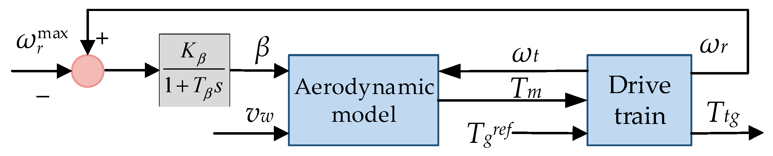
2.2. Wind Power System

The wind power system, as shown in Figure 3, is represented by a simplified variable speed wind turbine model. The model is mainly composed of an aerodynamic module and a drive train module. The aerodynamic module of the wind turbine is represented by a Cp (λ, β) curve as below [28]:
{ C p = c 0 ( c 1 1 λ i + c 2 β + c 3 ) e c 4 1 λ i + c 5 λ 1 λ i = 1 λ + b 0 β + b 1 β 3 + 1
where Cp and β are, respectively, the power coefficient and pitch angle; c0c5, b0, and b1 are constants. The values used for the simulations in this study are shown in Appendix B. The tip speed ratio λ is defined in (11):
λ = ω t R v w
P m = 0.5 ρ C P π R 2 v w 3
T m = P m ω t
where ωt, vw, and R are the rotating speed of wind rotor (rad/s), wind speed (m/s), and rotor radius (m), respectively; Pm and Tm are, respectively, the mechanical power and mechanical torque extracted by the rotor; ρ is the air density (kg/m3).
The drive train system is described as a two-mass system as below [27]:
{ ω ˙ t = 1 2 H t ( T m D t ω t D t g ( ω t ω r ) T t g ) T ˙ t g = K t g ( ω t ω r ) ω ˙ r = 1 2 H g ( T t g + D t g ( ω t ω r ) D g ω r T g r e f )
where ωr is the generator rotating speed; Ht and Hg are, respectively, the inertia constants of the wind turbine and generator; Dt, Dg, and Dtg are the mechanical damping coefficients of the wind turbine, generator, and flexible coupling, respectively; Ktg and Ttg are, respectively, the shaft stiffness and speed torque of the drive train; T g r e f is the generator braking electromotive torque. Baselines for normalizing the parameters in (14) are given in Appendix B.
The turbine dynamics described in (14) are listed in the following state-space form:
{ x ˙ w ( t ) = A w x w ( t ) + B w u w ( t ) + D w d w ( t ) y w ( t ) = C w x w ( t )
where xw = [ωt, Ttg, ωr]T is the state vector; uw = T g r e f is the control input; dw = Tm is the external disturbance; yw = ωt is the system output; the system matrices, Aw R3×3, Bw R3×1, Cw R1×3, Dw R3×1, are illustrated in Appendix A.
The pitch control system of the wind turbine is a PI controller as below [6]:
β = K β 1 + T β s ( ω r ω r max )
where Tβ and Kβ are a time constant and a proportionality constant, respectively; ω r max is the maximum value of ωr.

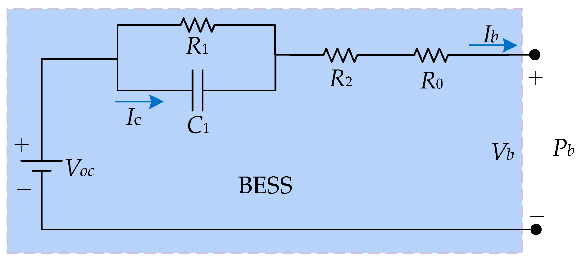
2.3. Battery Energy Storage System

A simplified equivalent circuit model is applied here to represent the dynamics of the BESS [29]. The model is shown in Figure 4. The capacitor current Ic (A), battery current Ib (A), and battery power output Pb (W) are selected as system states in this study. As a result, a nonlinear model of the BESS is obtained as below:
{ I ˙ c = 1 R 1 C 1 I c + u b + Δ U I ˙ b = u b P ˙ b = R 1 I c I ˙ b + V o c I ˙ b 2 ( R 0 + R 1 + R 2 ) I b I ˙ b + R 1 I b I ˙ c
where C1, R0, R1, and R2 are the capacitor and resistor parameters of the BESS. The values used for the simulations in this study are shown in Appendix B. ub is the control input representing the regulation amount on Ib; Voc is the open-circuit voltage; Vb is the battery voltage, and ∆U represents the system uncertainties of the BESS. As a nonlinear system, (17) cannot be converted to state-space form.
The power output Pb and state of charge (SoC) ς of the BESS are calculated as follows [29]:
P b = V b I b = R 1 I b I c + V o c I b ( R 0 + R 1 + R 2 ) I b 2
ς = 1 Q e / C b
Q e = Q e 0 + 0 t I b d t
where Cb is the battery capacity (Ah); Qe is the charge capacity at time t and Qe0 is the initial charge capacity. Qe0 is set to be 0.5Cb, so that the BESS has the same capacity for charge and discharge at the beginning. To ensure the BESS works in a safe range, a battery management system (BMS) is usually set to achieve safety constraints on Qe and Ib [46]. According to (19), the constraint on Qe is usually translated into the constraint on ς [31]. Thus, the safety constraints are [− I b max , I b max ] and [ςmin, ςmax]. Note that − I b max and I b max indicate the maximum charging current and maximum discharging current, respectively. In this study, the BMS is simplified to the following control logic (Algorithm 1) to realize the constraints on Ib and SoC:
Algorithm 1 Control logic of BMS
if SoC ∈[ςmin, ςmax]
  Ib ∈[− I b max , I b max ]
elseif SoC < ςmin
Ib ∈[0, I b max ]
elseif SoC > ςmax
  Ib ∈[− I b max , 0]
end

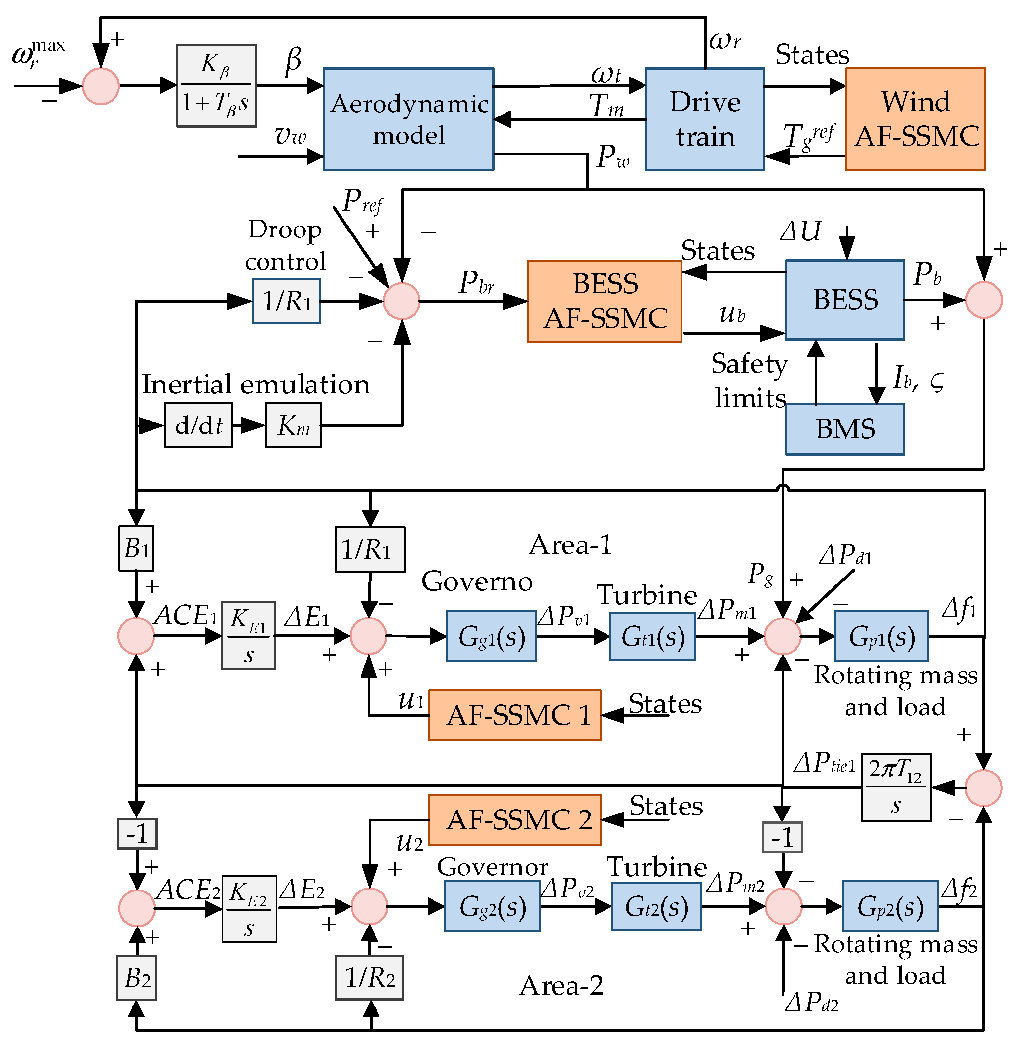
2.4. Hybrid Power System for Case Study

The control design in this study is applicable to power systems with different numbers of control areas. Without loss of generality, the hybrid power system in this study is a two-area thermal power system integrated with a wind farm and a BESS, as shown in Figure 5. The combined system of the wind farm and BESS is connected to Area-1. A comprehensive control framework is proposed for the hybrid power system: the wind farm maximizes its power output for better economic benefits, while the BESS is applied to compensate for the power deviations between the wind power output Pw and Pref; simultaneously, the BESS assists the thermal power system to improve frequency response through droop control and inertial emulation control. The reference power output of the BESS Pbr is calculated as follows:
P b r = P r e f P w Δ f 1 / R 1 K m d Δ f 1 / d t
where −∆f1/R1 and −Kmd∆f1/dt in (21) are the droop control term and the inertial emulation term [15], respectively. Km is a constant weighting the frequency deviation derivative.

3. Control Design

In this section, the controllers of the hybrid power system are designed based on the AF-SSMC method. To obtain good robustness against disturbances and uncertainties, we first design sliding functions and control laws for the subsystems according to their respective relative degrees. Then, the super-twisting algorithm is employed to achieve finite-time convergence and suppress system chattering. In addition, an adaptive fuzzy system is used to identify the controller gains and to adjust them adaptively online. The definition of relative degree is given below [47].
Definition 1. 
For a system whose output y is continuously derivable. The relative degree of the system is defined as the smallest derivative number n when the system input u appears in the nth derivative of y.

3.1. Control Design for the Power System

For the two-area power system shown in Figure 5, the control design of Area-1 is the same as that of Area-2. Considering the interactions between the subsystems, the external disturbance vectors of Area-1 and Area-2 are d1 = [Pg−∆P1, ∆f2]T and d2 = [−∆P2, ∆f1]T, respectively. The relative degree of the system represented by (9) is 3. Thus, the sliding function si of the ith control area is designed as below:
s i = c 1 i ( e i + e i j ) + c 2 i e ˙ i + e ¨ i
where c1i and c2i are positive constants satisfying that p2 + c2ip + c1i is Hurwitz, p is the Laplacian operator; ei = ∆fi−∆fir and eij = ∆Ptiei−∆Ptieir are the tracking errors of ∆fi and ∆Ptiei, respectively. The reference value of ∆fi and ∆Ptiei are, respectively, ∆fir = 0 and ∆Ptieir = 0.
The derivative of si is as follows:
s ˙ i = c 1 i e ˙ i j + c 1 i e ˙ i + c 2 i e ¨ i + e i
Substituting (4)–(8) into (23), then:
s ˙ i = a 1 i Δ f i + a 2 i Δ P m i + a 3 i Δ E i + a 4 i Δ P t i e i + a 5 i Δ P v i + φ i ( Δ P d i , Δ P ˙ d i , Δ P ¨ d i ) + b i u i
where a1i, a2i, a3i, a4i, a5i, and bi are functions of the system parameters, which are directly defined in (24). φi is the disturbance term, which is a function of ∆Pdi and ∆fj and their derivatives.
According to the super-twisting algorithm [37], we set:
s ˙ i = k 1 i | s i | sgn ( s i ) k 2 i sgn ( s i ) d τ
where the right side of the equation is the switching control law of the super-twisting SMC method; k1i and k2i are the control gains; sgn(si) is a symbolic function of si. Since SMC is insensitive to external disturbances and system uncertainties, φi is ignored in the control law design process to avoid additional disturbance observation. Combining (24) and (25), the control law of the ith control area ui is obtained as below:
u i = 1 b 1 i ( a 1 i Δ f i + a 2 i Δ P m i + a 3 i Δ E i + a 4 i Δ P t i e i + a 5 i Δ P v i + k 1 i | s i | sgn ( s i ) + k 2 i sgn ( s i ) d τ )
where the first five terms in (26) form the equivalent control law, and the last two terms form the switching control law.
It is complex to obtain optimal control gains through experience and simulation tests. Moreover, the effectiveness of the controller would be greatly affected without selecting proper gains. An adaptive fuzzy system is applied in this study to identify and adjust k1i and k2i online [38], which is constructed by the following process:
Step 1: We first construct fuzzy systems f ^ i ( s i | θ ^ f i ) and h ^ i ( s i | θ ^ h i ) to approximate the control gains k1i and k2i in (26), respectively. si is the input of the fuzzy systems. The fuzzy set of si is set with five elements. In this way, (26) is rewritten in the following form:
u i = 1 b 1 i ( a 1 i Δ f i + a 2 i Δ P m i + a 3 i Δ E i + a 4 i Δ P t i e i + a 5 i Δ P v i + f ^ i ( s i | θ ^ f i ) | s i | sgn ( s i ) + h ^ i ( s i | θ ^ h i ) sgn ( s i ) d τ )
where θ ^ f i R5×1 and θ ^ h i R5×1 are adjustable parameter sets of the two fuzzy systems, and they are adjusted according to adaptive laws.
Step 2: The fuzzy set of si is defined as A = {NB, NM, ZO, PM, PB}. NB, NM, ZO, PM, and PB are different evaluations of si representing negative big, negative middle, zero, positive middle, and positive big, respectively. The membership functions of si are defined in (28) and shown in Figure 6.
{ A N B ( s i ) = 1 / ( 1 + exp ( 5 ( s i + 3 ) ) ) A N M ( s i ) = exp ( ( s i + 2.5 ) 2 ) A Z O ( s i ) = exp ( s i 2 ) A P M ( s i ) = exp ( ( s i 2.5 ) 2 ) A P B ( s i ) = 1 / ( 1 + exp ( 5 ( s i 3 ) ) )
Step 3: The jth fuzzy rules are defined as below:
R(j): IF si is Aj THEN f ^ i is Fj and h ^ i is Hj
where Aj is the membership function of the jth item in the fuzzy set, j = 1, 2, …, 5. For example, A1 = ANB.
Step 4: Using product inference engine, singleton fuzzifier, and center average defuzzifier [38], the outputs of the fuzzy systems are obtained:
f ^ i ( s i | θ ^ f i ) = j = 1 5 y ¯ f j A j j = 1 5 A j , h ^ i ( s i | θ ^ h i ) = j = 1 5 y ¯ h j A j j = 1 5 A j
Let y ¯ f j and y ¯ h j be free parameters and set them as the parameters in the sets of θ ^ f i and θ ^ h i , respectively. Then, the outputs of the fuzzy systems in (29) are rewritten as:
{ f ^ i ( s i | θ ^ f i ) = θ ^ f i T ξ ( s i ) h ^ i ( s i | θ ^ h i ) = θ ^ h i T ξ ( s i )
where ξ(si) is the fuzzy basis vector as below:
ξ ( s i ) = [ A N B / j = 1 5 A j , A N M / j = 1 5 A j , A Z O / j = 1 5 A j , A P M / j = 1 5 A j , A P B / j = 1 5 A j ] T
Under the ideal case, f ^ i ( s i | θ f i ) = k 1 i and h ^ i ( s i | θ h i ) = k 2 i . θ f i and θ h i are, respectively, the optimal values of θ ^ f i and θ ^ h i defined as below:
{ θ f i = arg min θ ^ f i [ sup | f i ( s i | θ ^ f i ) k 1 i | ] θ h i = arg min θ ^ h i [ sup | h ^ i ( s i | θ ^ h i ) k 2 i | ]
Then, the deviations between θ ^ f i , θ ^ h i and their respective optimal values are defined as:
{ θ ˜ f i = θ f i θ ^ f i θ ˜ h i = θ h i θ ^ h i
Subsequently, the adaptive laws θ ^ ˙ f i , θ ^ ˙ h i of the fuzzy systems are derived through the Lyapunov stability theory to guarantee the ith control area with finite-time convergence and asymptotic stability.
Theorem 1. 
If the adaptive laws of the fuzzy systems are designed as (34) and the control gains satisfy k 1 i > 0 and k 2 i > | φ ˙ i | , the ith control area is guaranteed with finite-time convergence and asymptotic stability.
{ θ ^ ˙ f i = γ 1 | s i | ξ ( s i ) | s i | θ ^ ˙ h i = γ 2 s i ξ ( s i ) sgn ( s i ) d τ
where γ1 and γ2 are positive parameters.
Proof. 
The Lyapunov function of the ith control area is selected as:
V i = s i 2 / 2 + θ ˜ f i 2 / ( 2 γ 1 ) + θ ˜ h i 2 / ( 2 γ 2 )
Taking the derivative of Vi and then substituting (24)(27)(30)(33) into it:
V ˙ i = s i s ˙ i + θ ˜ f i θ ˜ ˙ f i / γ 1 + θ ˜ h i θ ˜ ˙ h i / γ 2 = s i ( a 1 i Δ f i + a 2 i Δ P m i + a 3 i Δ E i + a 4 i Δ P t i e i + a 5 i Δ P v i + φ i + b 1 i u i ) + θ ˜ f i θ ˜ ˙ f i / γ 1 + θ ˜ h i θ ˜ ˙ h i / γ 2 = s i [ φ i θ ^ f i ξ ( s i ) | s i | sgn ( s i ) θ ^ h i ξ ( s i ) sgn ( s i ) d τ ] + θ ˜ f i θ ˜ ˙ f i / γ 1 + θ ˜ h i θ ˜ ˙ h i / γ 2 = s i [ φ i θ ^ f i ξ ( s i ) | s i | sgn ( s i ) + θ f i ξ ( s i ) | s i | sgn ( s i ) θ f i ξ ( s i ) | s i | sgn ( s i ) θ ^ h i ξ ( s i ) sgn ( s i ) d τ + θ h i ξ ( s i ) sgn ( s i ) d τ + θ h i ξ ( s i ) sgn ( s i ) d τ ] + θ ˜ f i θ ˜ ˙ f i / γ 1 + θ ˜ h i θ ˜ ˙ h i / γ 2 = s i [ φ i θ ˜ f i ξ ( s i ) | s i | sgn ( s i ) k 1 i | s i | sgn ( s i ) θ ˜ h i ξ ( s i ) sgn ( s i ) d τ + k 2 i sgn ( s i ) d τ ] + θ ˜ f i θ ˜ ˙ f i / γ 1 + θ ˜ h i θ ˜ ˙ h i / γ 2
According to the adaptive laws designed in (34), (36) is modified into another form:
V ˙ i = s i [ φ i θ ˜ f i ξ ( s i ) | s i | sgn ( s i ) k 1 i | s i | sgn ( s i ) θ ˜ h i ξ ( s i ) sgn ( s i ) d τ + k 2 i sgn ( s i ) d τ ] + θ ˜ f i [ γ 1 | s i | ξ ( s i ) | s i | ] / γ 1 + θ ˜ h i [ γ 2 s i ξ ( s i ) sgn ( s i ) d τ ] / γ 2 = k 1 i | s i | | s i | k 2 i s i sgn ( s i ) d τ + s i φ i k 1 i | s i | | s i | | s i | k 2 i d τ + | s i | | φ ˙ i | d τ = k 1 i | s i | | s i | | s i | ( k 2 i d τ | φ ˙ i | d τ )
Since k 1 i > 0 and k 2 i > | φ ˙ i | have been given in Theorem 1, the inequality V ˙ i 0 is ensured to be true. Thus, the power system is guaranteed with asymptotic stability and finite-time convergence. That means, si will converge to 0 and then ei will also converge to 0 within finite time. □

3.2. Control Design for the Wind Power System

The maximum power point tracking (MPPT) strategy is the most common control strategy for variable-speed wind turbines to achieve maximum wind energy capture. According to the MPPT strategy, the wind turbine tracks the optimized generator rotating speed ω t o p t when vw is below the rated wind speed v w r a t e . From (11), ω t o p t is obtained as below:
ω t o p t = λ o p t v w R
where λopt is the optimized tip speed ratio. When vw is greater than v w r a t e , ωt is limited to its maximum value ω t m a x , and the power output of the wind turbine is limited to the rated capacity Prate by pitch control.
The relative degree of the system in (15) is 2 of which the sliding function sw is designed as below:
s w = c w e w + e ˙ w
where cw is a positive constant; ew = ωt ω t o p t is the tracking error. The derivative of sw is as follows:
s ˙ w = c w e ˙ w + e ¨ w = w 1 ω t + w 2 T t g + w 3 ω r c w ω ˙ t o p t ω ¨ t o p t w 4 u w + φ w ( T m , T ˙ m )
where w1, w2, w3, w4, and w5 are functions of the system parameters, which are directly defined in (40). The disturbance term φw is a function of Tm and its first derivative.
According to the super-twisting algorithm [37], we also set:
s ˙ w = k w 1 | s w | sgn ( s w ) k w 2 sgn ( s w ) d τ
where kw1 and kw2 are the control gains; ignoring φw and combining (40) and (41), the control law of the wind power system uw is obtained:
u w = ( w 1 ω t + w 2 T t g + w 3 ω r c w ω ˙ t o p t ω ¨ t o p t ) / w 4 + k w 1 | s w | sgn ( s w ) + k w 2 sgn ( s w ) d τ
where the first term in (42) is the equivalent control law, and the last two terms form the switching control law.
Based on the adaptive fuzzy system described in Section 3.1, an adaptive fuzzy system with the same structure is designed for the wind power system to identify and adjust kw1 and kw2 online. We denote the fuzzy systems of the wind power system as f w ( s w | θ ^ f w ) and h ^ w ( s w | θ ^ h w ) .
Theorem 2. 
If the adaptive laws of the fuzzy systems are designed as (43) and the control gains satisfy k w 1 > 0 and k w 2 > | φ ˙ w | , the wind power system is guaranteed with asymptotic stability and finite-time convergence.
{ θ ^ ˙ f w = γ 1 | s w | ξ ( s w ) | s w | θ ^ ˙ h w = γ 2 s w ξ ( s w ) sgn ( s w ) d τ
where ξ(sw) is the fuzzy basis vector of sw.
Proof. 
The Lyapunov function of the wind power system is selected as:
V w = s w 2 / 2 + θ ˜ f w 2 / ( 2 γ 1 ) + θ ˜ h w 2 / ( 2 γ 2 )
Equation (44) is in the same form as (35). Taking the derivative of Vw, it is easy to derive the inequality V ˙ w 0 through the same process in Theorem 1 and its proof. The specific proving process of Theorem 2 is no longer listed again for the sake of brevity. Therefore, the wind power system is guaranteed with finite-time convergence and asymptotic stability. That means, sw will converge to 0 and then ew will also converge to 0 within finite time. □

3.3. Control Design for the BESS

The system dynamics of the BESS are described in (17). Different from the other subsystems of the hybrid power system, the BESS is a nonlinear system of which the relative degree is 2. xb = [Ic, Ib, Pb]T is the state vector of the BESS. yb = Pb is the system output. The sliding function sb of the BESS is designed as below:
s b = e b + c b e b d t
where cb is a positive constant; eb = PbPbr is the tracking error. The derivative of sb is as follows:
s ˙ = e ˙ + c b e b = P ˙ P ˙ d + c b e b = [ R 1 I c + E m ( 2 R 0 + R 1 + 2 R 2 ) I b ] u b I b I c / C 1 + R 1 I b Δ U P ˙ d + c b e b
According to the super-twisting algorithm [37], we set:
s ˙ b = k b 1 | s b | sgn ( s b ) k b 2 sgn ( s b ) d τ
where kb1 and kb2 are the control gains. Ignoring the disturbance term R1IbU and combining (46) and (47), the control law of the BESS ub is obtained:
u b = I b I c / C 1 c b e b + P ˙ d k b 1 | s b | sgn ( s b ) k b 2 sgn ( s b ) d τ R 1 I c + E m ( 2 R 0 + R 1 + 2 R 2 ) I b
where the first three terms in (48) form the equivalent control law, and the last two terms form the switching control law.
Based on the adaptive fuzzy system described in Section 3.1, an adaptive fuzzy system with the same structure is also designed for the BESS to identify and adjust kb1 and kb2 online. We denote the fuzzy systems of the BESS as f b ( s b | θ ^ f b ) and h ^ b ( s b | θ ^ h b ) .
Theorem 3. 
If the adaptive laws of the fuzzy systems are designed as (49) and the control gains satisfy k b 1 > 0 and k b 2 > | R 1 I b Δ U | , the BESS is guaranteed with finite-time convergence and asymptotic stability.
{ θ ^ ˙ f b = γ 1 | s b | ξ ( s b ) | s b | θ ^ ˙ h b = γ 2 s b ξ ( s b ) sgn ( s b ) d τ
where ξ(sb) is the fuzzy basis vector of sb.
Proof. 
The Lyapunov function of the BESS is selected as:
V b = s b 2 / 2 + θ ˜ f b 2 / ( 2 γ 1 ) + θ ˜ h b 2 / ( 2 γ 2 )
Equation (50) is also in the same form as (35). Taking the derivative of Vb, it is easy to derive the inequality V ˙ b 0 through the same process in Theorem 1 and its proof. Hence, the proving process of Theorem 3 is also omitted. Therefore, the BESS is guaranteed with asymptotic stability and finite-time convergence. That means, sb will converge to 0 and then eb will also converge to 0 within finite time. □
So far, the asymptotic stability of each subsystem has been proved through the Lyapunov stability theory. The states of the wind power system and BESS are not directly affected by other subsystems. The link between the BESS and other subsystems is the tracking of Pbr to assist in frequency regulation and wind power smoothing. For the entire hybrid system shown in Figure 5, the direct state impact between subsystems lies in the two-area power system and includes two aspects: (a) the power output of the combined system Pg is integrated into area-1; (b) each area receives the influence of the frequency deviation in the other area through the tie line. These interactions are considered as shown in Section 3.1 when defining the external disturbances of Area-1 and Area-2. Therefore, when the asymptotic stability of each subsystem is guaranteed, the asymptotic stability of the hybrid power system is also guaranteed.

4. Numerical Simulations

To evaluate the effectiveness of the developed control framework, simulation experiments are conducted on the hybrid power system in this section through MATLAB/Simulink. The wind power system here represents a wind farm consisting of 10 wind turbines. The rated power output of each wind turbine is 1.5 MW. The size of the BESS is 2 MWh. A series of lead-acid batteries (specifications of a single battery: 2.135 V–500 Ah) can be used to realize it [29]. Specifically, 438 batteries are connected in series to get the rated capacity at 1000 V dc-link voltage, and 4 of such series are connected in parallel to obtain the energy rating. The constraint on the BESS current is set as [−2000 A, 2000 A], and the constraint on SOC is set as [20%, 80%] [31]. Both Area-1 and Area-2 have an installed thermal power capacity of 50 MW. The control gains are selected as c11 = 2500, c12 = 100, c21 = 100, c22 = 20, cw = cb = 2, γ1 = γ2 = 20. Other system parameters are listed in Appendix B.

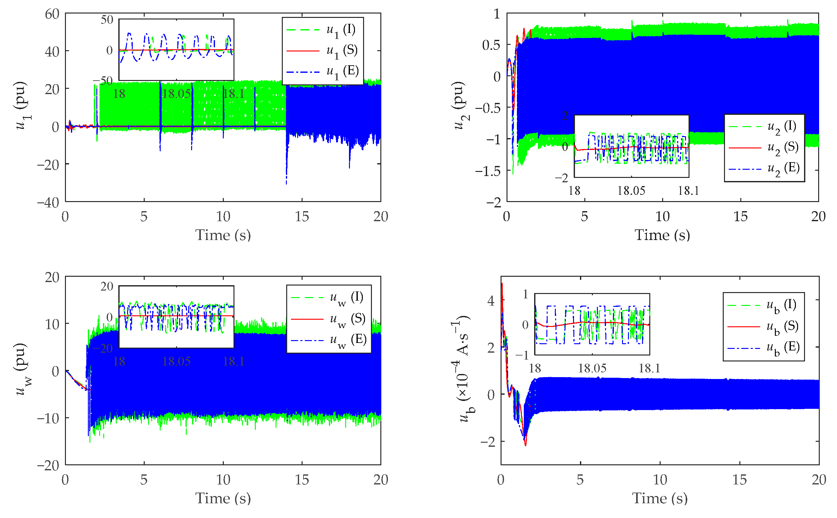
4.1. Control Properties with/without Super-Twisting Algorithm

The control properties of the AF-SSMC method are tested in the first simulation experiment. For comparison, the super-twisting reaching law (S) in (25), (41), and (47) is replaced by the conventional exponential reaching law (E) and its practical special case [35], the isokinetic reaching law (I), as follows:
Isokinetic   reaching   law :   s ˙ = ε 1 sgn ( s )   ε 1 > 0
Exponential   reaching   law :   s ˙ = ε 2 sgn ( s ) δ s   ε 2 > 0 , δ > 0
where ε1, ε2, and δ are control gains that are approximated by the adaptive fuzzy system as described in Section 3.1.
In this experiment, the external disturbances and system uncertainties are set as vw = 10 m/s, ∆Pd1 = ∆Pd2 = 0.01 (pu), ∆U = 0.01 (pu); the reference power of the wind farm is Pref = 8.85 MW. The results are shown in Figure 7 and Figure 8. The outputs of the subsystems are presented in Figure 7. On the whole, the system outputs under different reaching laws converge to their respective target values similarly, owing to the designed sliding functions. With the compensation of the BESS, the power outputs Pg of the wind-BESS combined system are able to achieve the tracking of Pref under the three reaching laws, and the frequency deviations converge to near 0. Closer inspection shows that the super-twisting reaching law reduces the tracking errors of the two-area power system (shown in the enlarged views in Figure 7), although with a slight overshoot and a slightly longer convergence time.
The control signals of the subsystems are shown in Figure 8. All of the control signals under the super-twisting reaching law are much more stable than those under the other two reaching laws. This indicates that the application of the super-twisting algorithm effectively reduces the chattering of the sliding mode control law. Under constant disturbances, the control chattering of the AF-SSMC is almost negligible when the subsystems are stable.

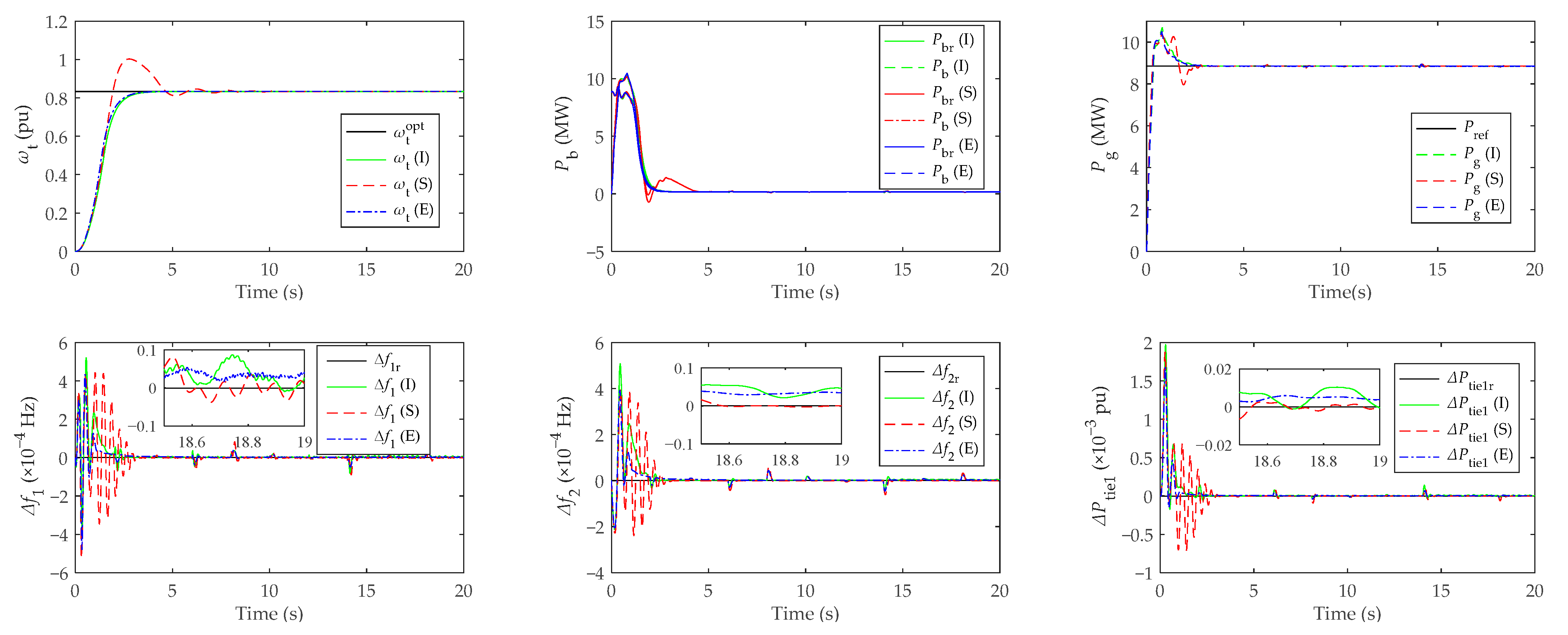
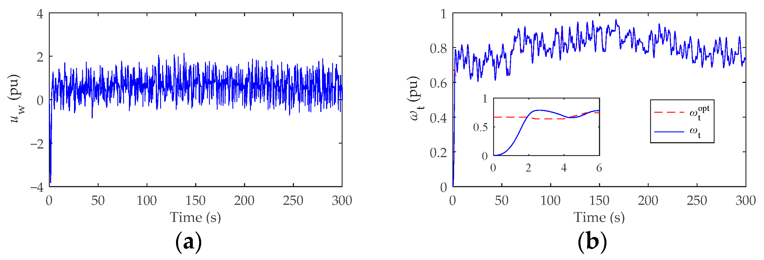
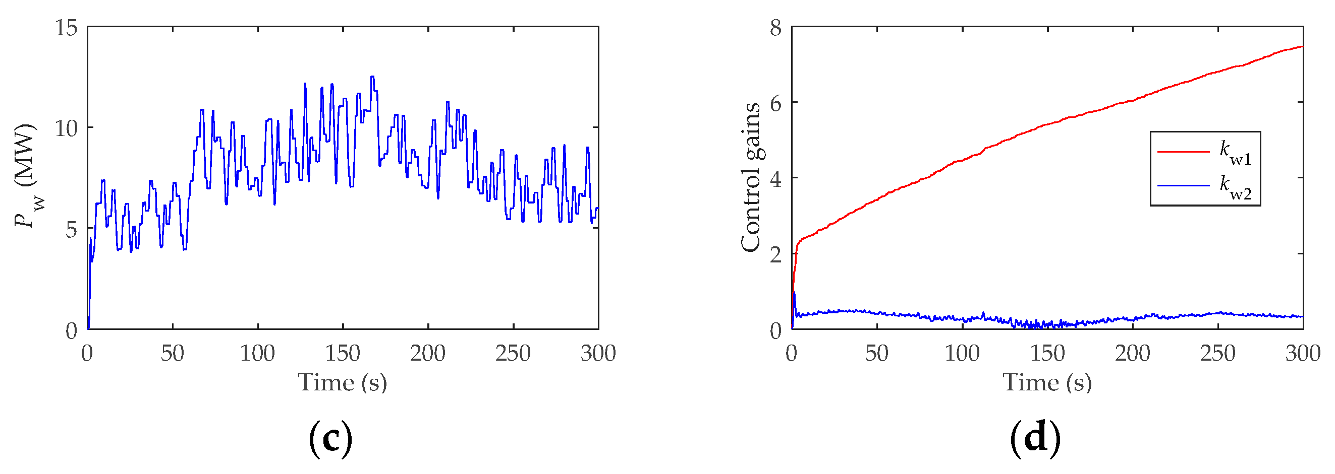
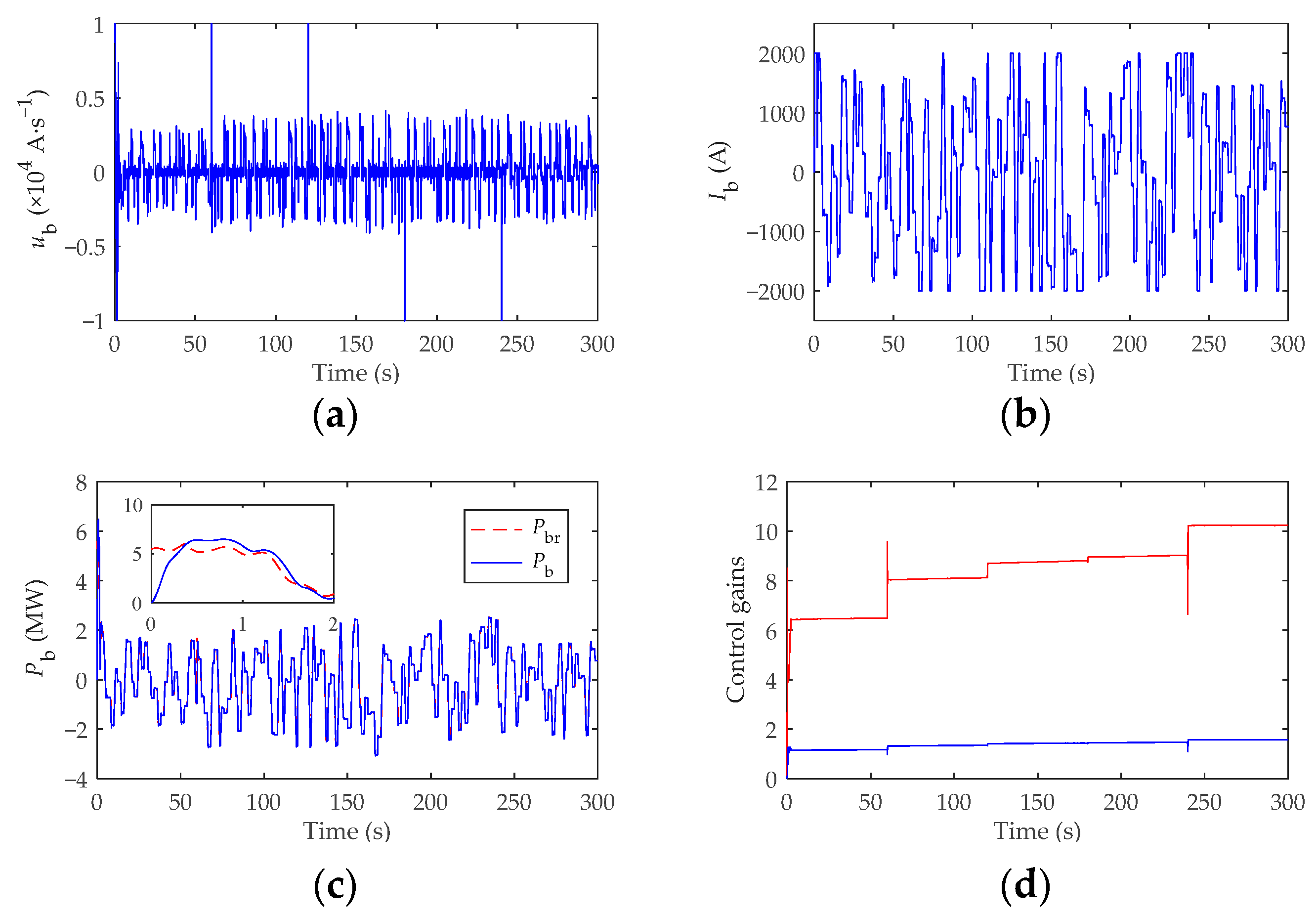
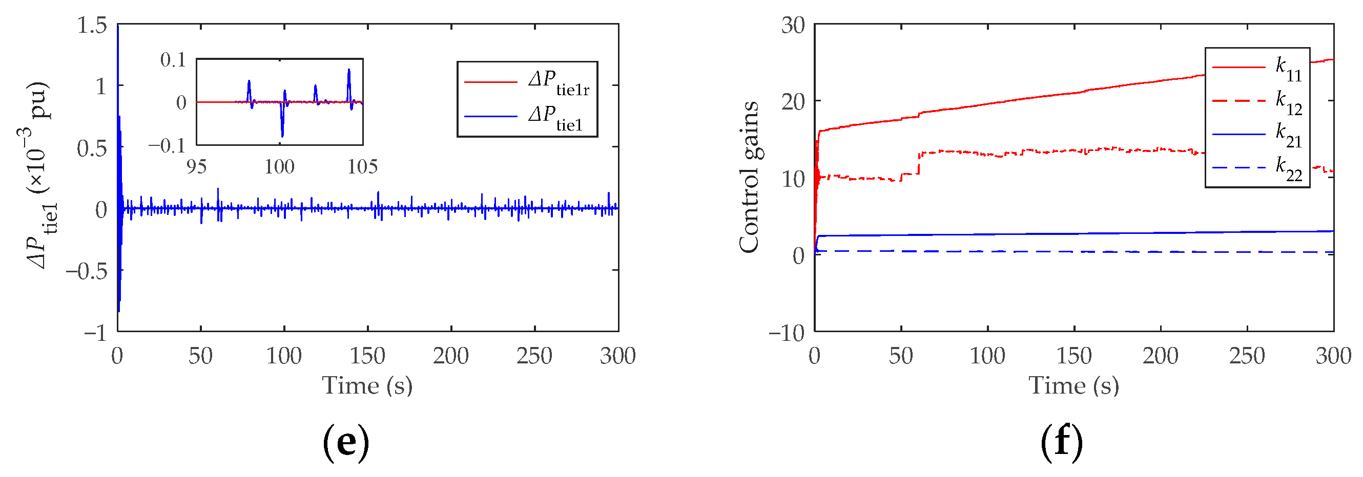
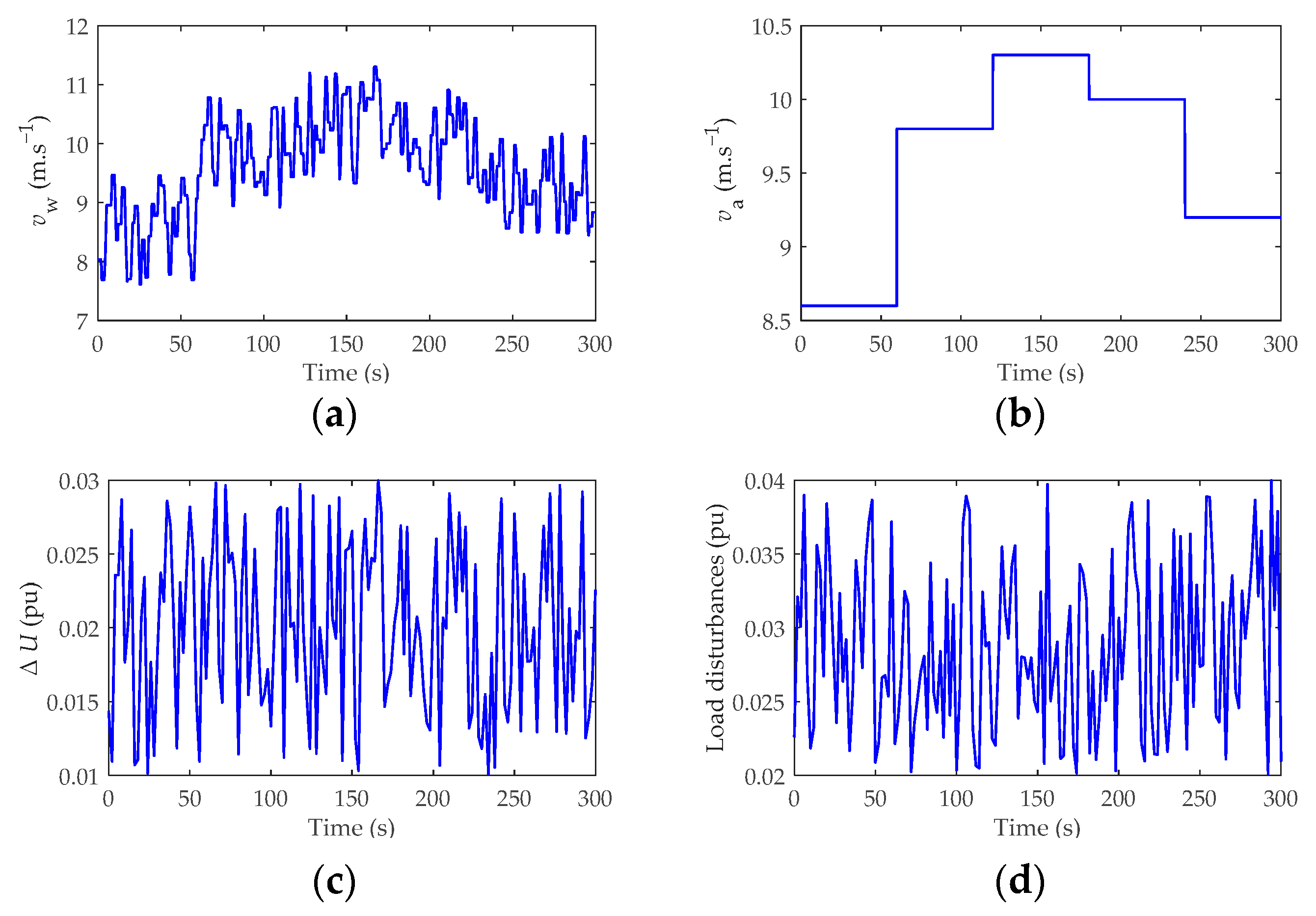
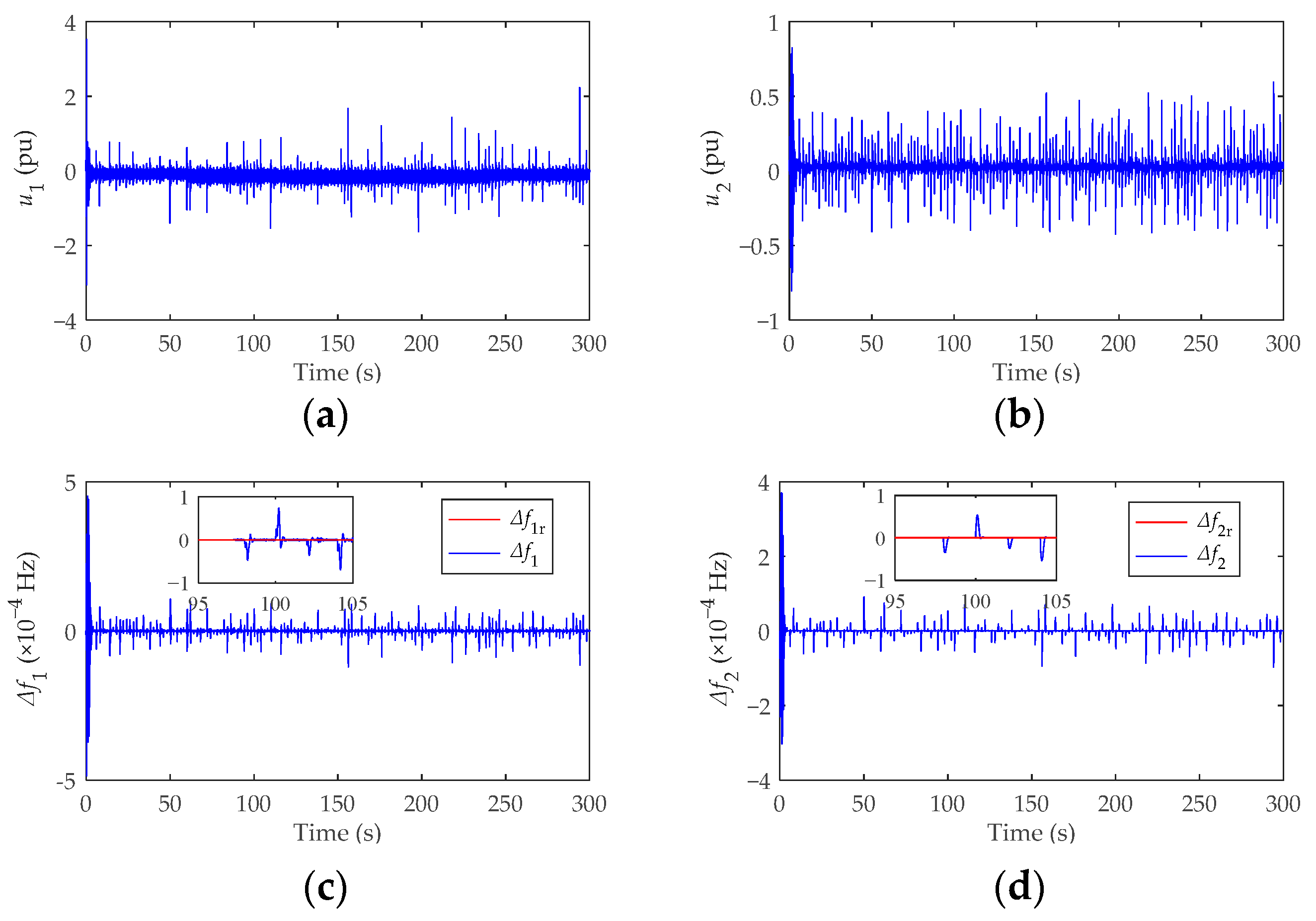
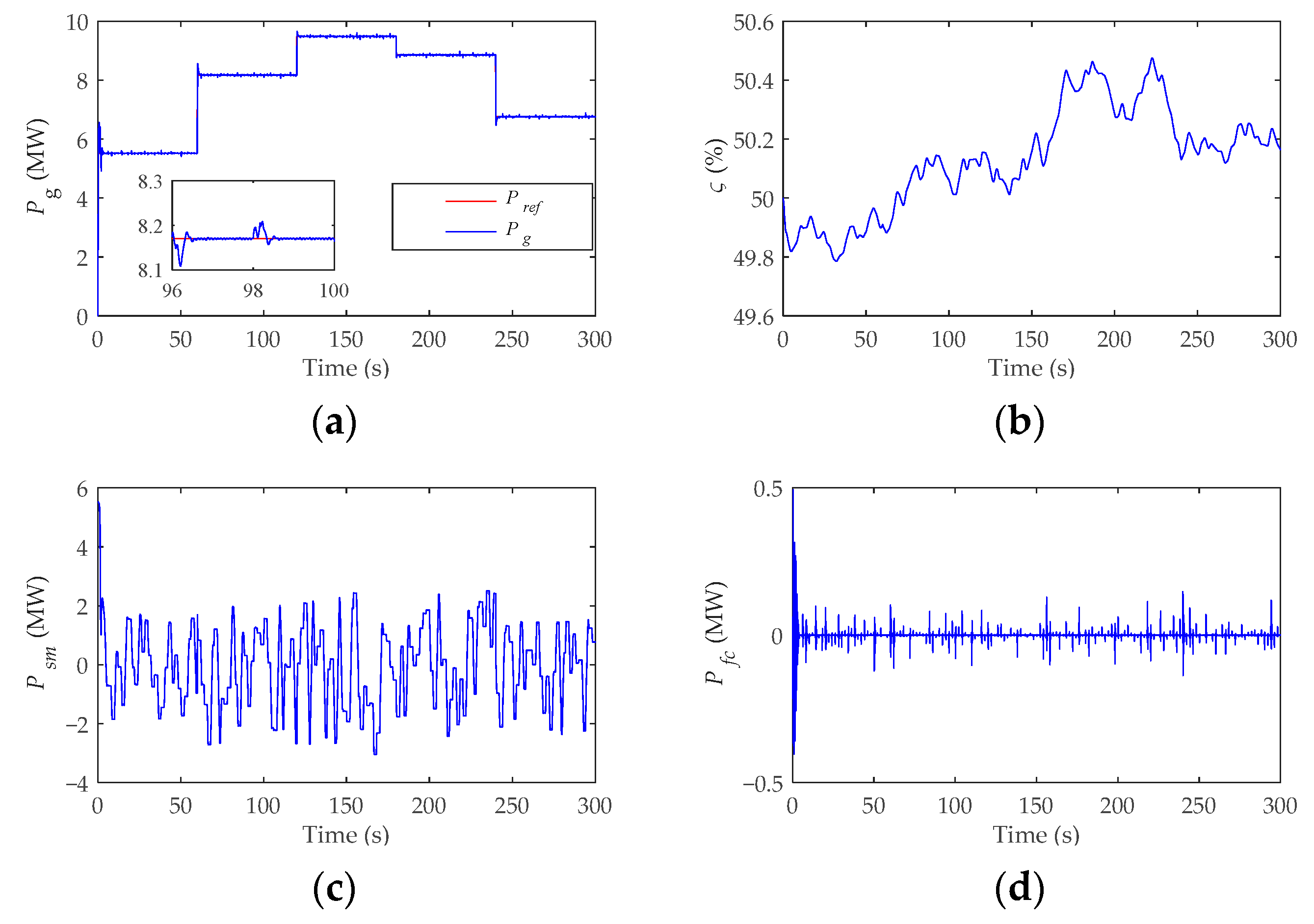
4.2. Dynamic Analysis on Frequency Regulation and Wind Power Smoothing

To test the effectiveness and robustness of the proposed control framework, the second simulation is carried out under the dynamic external disturbances and system uncertainties as presented in Figure 9. The wind speed is shown in Figure 9a of which the average value per minute va is shown in Figure 9b. Figure 9c shows the system uncertainties of the BESS. The load disturbances ∆Pd1 and ∆Pd2 are set to be the same signal shown in Figure 9d.
The results of the second simulation are shown in Figure 10, Figure 11, Figure 12 and Figure 13. Figure 10 presents the response process of the wind power system. It can be seen that the tracking of ωt is performed with high accuracy with the help of the designed AF-SSMC controller. Resulting from the rapid variations of wind speed, fluctuations appear in the control signal uw. The power output of the wind farm is shown in Figure 10c, which is generated according to the MPPT strategy. Figure 10d shows the approximate processes of kw1 and kw2.
Figure 11 presents the response process of the BESS. Though fluctuations appear in the control signal ub due to the external disturbances and system uncertainties, Pb tracks its reference value Pbr with high accuracy. It can be seen that Ib varies within the set limit during the process. The approximate processes of kb1 and kb2 are shown in Figure 11d.
The behavior of the two-area thermal power system is presented in Figure 12. Fluctuations also appear in the responses of the two-area power system due to the external disturbances and system uncertainties. Besides the load disturbance, Area-1 is simultaneously interfered by Pg. Thus, the amplitude of u1 is significantly larger than that of u2. Even though affected by the disturbances and uncertainties, the designed controllers manage to keep the frequency deviations and tie-line power flow at approximately 0. Nevertheless, the enlarged views show that the fluctuations in ∆f1, ∆f2, and ∆Ptie1 smooth down quickly. The approximate processes of k11, k12, k21, and k22 are shown in Figure 12f.
Figure 13 illustrates the power variation process of the BESS involved in wind power smoothing and frequency control. Figure 13a shows the tracking process of Pg, where Pref is set according to the average wind speed per minute shown in Figure 9b and the MPPT strategy. It can be seen that Pg effectively implements the tracking of Pref to smooth the wind power output during this process, despite the continuous fluctuations in Pw (as shown in Figure 10c). During the process, the SoC of the BESS only varies in a small range within the set constraint. Figure 13c,d show the parts of Pbr (displayed in Figure 11c) for wind power smoothing Psm and frequency control Pfc, respectively. According to (21), they are calculated as follows:
P s m = P r e f P w
P f c = Δ f 1 / R 1 K m d Δ f 1 / d t
The participation in frequency control of the BESS does not significantly reduce its tracking accuracy to Pg. By comparing Figure 13a,b, it can be explained by the fact that the required power from the BESS for frequency control is much smaller than that for compensating for the deviation between Pw and Pref.

5. Conclusions

This study set out to reduce the adverse effects of fluctuating wind power on the stability and safety of the power system. To this end, a comprehensive control framework is proposed, which simultaneously utilizes the BESS for LFC and wind power smoothing. The controllers of the subsystems are designed based on the AF-SSMC method. The simulations verify the effectiveness and robustness of the proposed control framework to maintain the stable operation of the hybrid power system. In addition, it can be found that the participation in frequency regulation of the BESS does not significantly reduce the tracking accuracy of the reference power from TSO.
The frequent charging and discharging actions of the BESS would shorten its lifetime, which is not considered in this study. Future works might focus on different coordinated control methods between the wind power system and BESS to extend the BESS lifetime.
Due to the sensor measurement, there may be errors or delays in the measured states in practical applications, which will reduce the actual control effect of the controller. These factors were not considered in the simulation analysis of this study, and the measured signal can be corrected by designing a suitable state observer in the future.

Author Contributions

Z.D.: data curation, methodology, writing—original draft preparation, software; C.X.: conceptualization, funding acquisition, resources, supervision; Z.H.: software, validation; X.H.: visualization, investigation; F.X.: writing—review and editing. All authors have read and agreed to the published version of the manuscript.

Funding

This research was funded by the National Natural Science Foundation of China, grant number No. 52106238, the Fundamental Research Funds for the Central Universities, grant number No. B210201018, and the Post-graduate Research & Practice Innovation Program of Jiangsu Province, grant number No. KYCX21_0520.

Data Availability Statement

Not applicable.

Conflicts of Interest

The authors declare no conflict of interest. The funders had no role in the design of the study; in the collection, analyses, or interpretation of data; in the writing of the manuscript; or in the decision to publish the results.

Appendix A. System Matrices

(1) System matrices of the ith control area
A i = [ 1 T p i K p i T p i 0 K p i T p i 0 0 1 T c h i 0 0 1 T c h i K E i B i 0 0 K E i 0 2 π T i j 0 0 0 0 1 R i T g i 0 1 T g i 0 1 T g i ] ,   B i = [ 0 0 0 0 1 T g i ] T D i = [ K p i T p i 0 0 0 0 0 0 0 2 π T i j 0 ] T C i = [ 1 0 0 0 0 ]
(2) System matrices of the wind power system
A w = [ ( D t + D t g ) 2 H t K t g D t g 2 H g 1 2 H t 0 1 2 H g D t g 2 H t K t g ( D g + D t g ) 2 H g ] , B w = [ 0 0 1 2 H g ] ,   D w = [ 1 2 H t 0 0 ] , C w = [ 0 0 1 ] T , x w = [ ω t T t g ω r ]

Appendix B. System Parameters

(1) Parameters of the ith control area [27]
Tch1 = 0.3, Tch2 = 0.17, Kp1 = 1, Kp2 = 0.67, Tp1 = 10, Tp2 = 8, Tg1 = 0.1, Tg2 = 0.4, R1 = R2 = 0.05, B1 = 41, B2 = 81.5, KE1 = 0.5, KE2 = 0.5, T12 = 3.77.
(2) Parameters of the wind power system
Prate = 1.5 MW, R = 30 m, ω t m a x = 3.17 rad/s, λopt = 8.1, v w r a t e = 12 m/s, Kβ = 1, Tβ = 0.5, Ht = 2.49 s, Hg = 0.9 s, Dtg = 1.5, Dt = Dg = 0, Ktg = 296.7 pu.
Baselines for normalization: ω t b = 3.17 rad/s, ω r b =nt ω t b , nt = 50 is the gearbox ratio; Tb = Prate/ ω t b .
Parameters of the Cp (λ, β) curve: c0 = 0.5176, c1 = 116, c2 = −0.4, c3 = −5, c4 = −21, c5 = 0.0068, b0 = 0.08, b1 = −0.035.
(3) Parameters of the BESS
Voc = 2.041 V, C1 = 12195121 pF, R1 = 0.00041 Ω, R2 = 0.0002 Ω, R0 = 0.00168 Ω.

References

  1. Khalid, M.; Aguilera, R.P.; Savkin, A.V.; Agelidis, V.G. On maximizing profit of wind-battery supported power station based on wind power and energy price forecasting. Appl. Energy 2018, 211, 764–773. [Google Scholar] [CrossRef]
  2. Wang, B.; Zhou, M.; Xin, B.; Zhao, X.; Watada, J. Analysis of operation cost and wind curtailment using multi-objective unit commitment with battery energy storage. Energy 2019, 178, 101–114. [Google Scholar] [CrossRef]
  3. Nguyen, N.; Mitra, J. An Analysis of the Effects and Dependency of Wind Power Penetration on System Frequency Regulation. IEEE Trans. Sustain. Energy 2016, 7, 354–363. [Google Scholar] [CrossRef]
  4. Latif, A.; Hussain, S.M.S.; Das, D.C.; Ustun, T.S. State-of-the-art of controllers and soft computing techniques for regulated load frequency management of single/multi-area traditional and renewable energy based power systems. Appl. Energy 2020, 266, 114858. [Google Scholar] [CrossRef]
  5. Ansari, J.; Reza Abbasi, A.; Bahmani Firouzi, B. Decentralized LMI-based event-triggered integral sliding mode LFC of power systems with disturbance observer. Int. J. Electr. Power Energy Syst. 2022, 138, 107971. [Google Scholar] [CrossRef]
  6. Pradhan, C.; Bhende, C.N.; Samanta, A.K. Adaptive virtual inertia-based frequency regulation in wind power systems. Renew. Energy 2018, 115, 558–574. [Google Scholar] [CrossRef]
  7. Kumar, N.K.; Gopi, R.S.; Kuppusamy, R.; Nikolovski, S.; Teekaraman, Y.; Vairavasundaram, I.; Venkateswarulu, S. Fuzzy Logic-Based Load Frequency Control in an Island Hybrid Power System Model Using Artificial Bee Colony Optimization. Energies 2022, 15, 2199. [Google Scholar] [CrossRef]
  8. Wang, X.; Wang, Y.; Liu, Y. Dynamic load frequency control for high-penetration wind power considering wind turbine fatigue load. Int. J. Electr. Power Energy Syst. 2020, 117, 105696. [Google Scholar] [CrossRef]
  9. Behera, A.; Panigrahi, T.K.; Ray, P.K.; Sahoo, A.K. A Novel Cascaded PID Controller for Automatic Generation Control Analysis With Renewable Sources. IEEE/CAA J. Autom. Sin. 2019, 6, 1438–1451. [Google Scholar] [CrossRef]
  10. Sun, Y.; Wang, Y.; Wei, Z.; Sun, G.; Wu, X. Robust H∞ load frequency control of multi-area power system with time delay: A sliding mode control approach. IEEE/CAA J. Autom. Sin. 2018, 5, 610–617. [Google Scholar] [CrossRef]
  11. Anand, S.; Dev, A.; Sarkar, M.K. Generalized proportional integral observering mode control approach. IEEE/CAA J. Autom. Sin. 2018, 5, 610–617, IEEE/CAA J. Autom. Sin.2019, 6, 1438–1451. [Google Scholar]
  12. Guo, J. Application of full order sliding mode control based on different areas power system with load frequency control. ISA Trans. 2019, 92, 23–34. [Google Scholar] [CrossRef] [PubMed]
  13. Jena, N.K.; Sahoo, S.; Sahu, B.K.; Ranjan Nayak, J.; Mohanty, K.B. Fuzzy adaptive selfish herd optimization based optimal sliding mode controller for frequency stability enhancement of a microgrid. Eng. Sci. Technol. 2022, 33, 101071. [Google Scholar] [CrossRef]
  14. Lamsal, D.; Sreeram, V.; Mishra, Y.; Kumar, D. Output power smoothing control approaches for wind and photovoltaic generation systems: A review. Renew. Sustain. Energy Rev. 2019, 113, 109245. [Google Scholar] [CrossRef]
  15. Xue, Y.; Tai, N. Review of contribution to frequency control through variable speed wind turbine. Renew. Energy 2011, 36, 1671–1677. [Google Scholar]
  16. Abouzeid, S.I.; Guo, Y.; Zhang, H.-C. Cooperative control framework of the wind turbine generators and the compressed air energy storage system for efficient frequency regulation support. Int. J. Electr. Power Energy Syst. 2021, 130, 106844. [Google Scholar] [CrossRef]
  17. De Siqueira, L.M.S.; Peng, W. Control strategy to smooth wind power output using battery energy storage system: A review. J. Energy Storage 2021, 35, 102252. [Google Scholar] [CrossRef]
  18. Datta, U.; Kalam, A.; Shi, J. The relevance of large-scale battery energy storage (BES) application in providing primary frequency control with increased wind energy penetration. J. Energy Storage 2019, 23, 9–18. [Google Scholar] [CrossRef]
  19. Zhao, H.; Wu, Q.; Hu, S.; Xu, H.; Rasmussen, C.N. Review of energy storage system for wind power integration support. Appl. Energy 2015, 137, 545–553. [Google Scholar] [CrossRef]
  20. Hauer, I.; Balischewski, S.; Ziegler, C. Design and operation strategy for multi-use application of battery energy storage in wind farms. J. Energy Storage 2020, 31, 101572. [Google Scholar] [CrossRef]
  21. Lamsal, D.; Sreeram, V.; Mishra, Y.; Kumar, D. Smoothing control strategy of wind and photovoltaic output power fluctuation by considering the state of health of battery energy storage system. IET Renew. Power Gener. 2019, 13, 578–586. [Google Scholar] [CrossRef]
  22. Cao, M.; Xu, Q.; Qin, X.; Cai, J. Battery energy storage sizing based on a model predictive control strategy with operational constraints to smooth the wind power. Int. J. Electr. Power Energy Syst. 2020, 115, 105471. [Google Scholar] [CrossRef]
  23. Wan, C.; Qian, W.; Zhao, C.; Song, Y.; Yang, G. Probabilistic Forecasting Based Sizing and Control of Hybrid Energy Storage for Wind Power Smoothing. IEEE Trans. Sustain. Energy 2021, 12, 1841–1852. [Google Scholar] [CrossRef]
  24. Khalid, M.; Savkin, A.V. Minimization and control of battery energy storage for wind power smoothing: Aggregated, distributed and semi-distributed storage. Renew. Energy 2014, 64, 105–112. [Google Scholar] [CrossRef]
  25. Guo, J. Application of a novel adaptive sliding mode control method to the load frequency control. Eur. J. Control. 2021, 57, 172–178. [Google Scholar] [CrossRef]
  26. Lv, X.; Sun, Y.; Wang, Y.; Dinavahi, V. Adaptive event-triggered load frequency control of multi-area power systems under networked environment via sliding mode control. IEEE Access 2020, 8, 86585. [Google Scholar] [CrossRef]
  27. Prasad, S.; Purwar, S.; Kishor, N. Non-linear sliding mode control for frequency regulation with variable-speed wind turbine systems. Int. J. Electr. Power Energy Syst. 2019, 107, 19–33. [Google Scholar] [CrossRef]
  28. Deng, Z.; Xu, C. Frequency Regulation of Power Systems with a Wind Farm by Sliding-Mode-Based Design. IEEE/CAA J. Autom. Sin. 2022, 9, 1980–1989. [Google Scholar] [CrossRef]
  29. Teleke, S.; Baran, M.E.; Bhattacharya, S.; Huang, A.Q. Optimal Control of Battery Energy Storage for Wind Farm Dispatching. IEEE Trans. Energy Convers. 2010, 25, 787–794. [Google Scholar] [CrossRef]
  30. Liu, K.; Wei, Z.; Zhang, C.; Shang, Y.; Teodorescu, R.; Han, Q.-L. Towards long lifetime battery: AI-based manufacturing and management. IEEE/CAA J. Autom. Sin. 2022, 9, 1139–1165. [Google Scholar] [CrossRef]
  31. Li, J.; Liu, K.; Zhou, Q.; Meng, J.; Ge, Y.; Xu, H. Electrothermal Dynamics-Conscious Many-Objective Modular Design for Power-Split Plug-in Hybrid Electric Vehicles. IEEE/ASME Trans. Mechatron. 2022, 1–11. [Google Scholar]
  32. Gohari, H.D.; Zarastvand, M.R.; Talebitooti, R.; Loghmani, A.; Omidpanah, M. Radiated sound control from a smart cylinder subjected to piezoelectric uncertainties based on sliding mode technique using self-adjusting boundary layer. Aerosp. Sci. Technol. 2020, 106, 106141. [Google Scholar] [CrossRef]
  33. Chen, D.; Zhang, J.; Li, Z. A Novel Fixed-Time Trajectory Tracking Strategy of Unmanned Surface Vessel Based on the Fractional Sliding Mode Control Method. Electronics 2022, 11, 726. [Google Scholar] [CrossRef]
  34. Wang, Y.; Feng, Y.; Zhang, X.; Liang, J. A New Reaching Law for Antidisturbance Sliding-Mode Control of PMSM Speed Regulation System. IEEE Trans. Power Electron. 2020, 35, 4117–4126. [Google Scholar] [CrossRef]
  35. Wang, D.; Wang, D.; Zhou, W.; Niu, L. Research on PMSM Sliding-mode Vector Combined Speed Controller Based on Improved Exponential Reaching Law. J. Phys. Conf. Ser. IOP Publ. 2022, 2260, 012024. [Google Scholar] [CrossRef]
  36. Guo, J. The Load Frequency Control by Adaptive High Order Sliding Mode Control Strategy. IEEE Access 2022, 10, 25392–25399. [Google Scholar] [CrossRef]
  37. Mirzaei, M.J.; Hamida, M.A.; Plestan, F.; Taleb, M. Super-twisting sliding mode controller with self-tuning adaptive gains. Eur. J. Control. 2022, 68, 100690. [Google Scholar] [CrossRef]
  38. Fei, J.; Feng, Z. Adaptive Fuzzy Super-Twisting Sliding Mode Control for Microgyroscope. Complexity 2019, 2019, 6942642. [Google Scholar] [CrossRef]
  39. Li, M.; Li, Y.; Wang, Q. Adaptive fuzzy backstepping super-twisting sliding mode control of nonlinear systems with unknown hysteresis. Asian J. Control. 2021, 24, 1726–1743. [Google Scholar] [CrossRef]
  40. Ren, H.; Zhang, L.; Su, C. Tracking control of an uncertain heavy load robot based on super twisting sliding mode control and fuzzy compensator. Asian J. Control. 2021, 24, 3190–3199. [Google Scholar] [CrossRef]
  41. Luo, W.; Zhao, T.; Li, X.; Wang, Z.; Wu, L. Adaptive super-twisting sliding mode control of three-phase power rectifiers in active front end applications. IET Control. Theory Appl. 2019, 13, 1483–1490. [Google Scholar] [CrossRef]
  42. Shen, J.; Dong, X.; Zhu, J.; Liu, C.; Wang, J. HOSMD and neural network based adaptive super-twisting sliding mode control for permanent magnet synchronous generators. Energy Rep. 2022, 8, 5987–5999. [Google Scholar] [CrossRef]
  43. Zaare, S.; Soltanpour, M.R. Adaptive fuzzy global coupled nonsingular fast terminal sliding mode control of n-rigid-link elastic-joint robot manipulators in presence of uncertainties. Mech. Syst. Signal Process. 2022, 163, 108165. [Google Scholar] [CrossRef]
  44. Ayas, M.S.; Altas, I.H. Fuzzy logic based adaptive admittance control of a redundantly actuated ankle rehabilitation robot. Control. Eng. Pract. 2017, 59, 44–54. [Google Scholar] [CrossRef]
  45. Li, P.; Jiao, X.; Li, Y. Adaptive real-time energy management control strategy based on fuzzy inference system for plug-in hybrid electric vehicles. Control. Eng. Pract. 2021, 107, 104703. [Google Scholar] [CrossRef]
  46. Rosewater, D.M.; Copp, D.A.; Nguyen, T.A.; Byrne, R.H.; Santoso, S. Battery Energy Storage Models for Optimal Control. IEEE Access 2019, 7, 178357–178391. [Google Scholar] [CrossRef]
  47. Chiu, C.-S. Derivative and integral terminal sliding mode control for a class of MIMO nonlinear systems. Automatica 2012, 48, 316–326. [Google Scholar] [CrossRef]
Figure 1. Hybrid power system with N areas.
Machines 10 01225 g001
Figure 2. Model of the ith control area.
Machines 10 01225 g002
Figure 3. Wind power system.
Machines 10 01225 g003
Figure 4. Equivalent circuit model of the BESS.
Machines 10 01225 g004
Figure 5. Hybrid power system.
Machines 10 01225 g005
Figure 6. Membership functions of si.
Machines 10 01225 g006
Figure 7. System outputs under different reaching laws.
Machines 10 01225 g007
Figure 8. Control signals under different reaching laws.
Machines 10 01225 g008
Figure 9. External disturbances and system uncertainties (a) Wind speed vw. (b) Average wind speed per minute va. (c) System uncertainties of the BESS ∆U. (d) Load disturbances ∆Pd1 and ∆Pd2.
Machines 10 01225 g009
Figure 10. Results of wind power system (a) Control input uw. (b) Tracking of the rotating speed ωt. (c) Power output Pw. (d) Control gains kw1 and kw2.
Machines 10 01225 g010aMachines 10 01225 g010b
Figure 11. Results of BESS (a) Control input ub. (b) Battery current Ib. (c) Tracking of the power output Pb. (d) Control gains kb1 and kb2.
Machines 10 01225 g011
Figure 12. Results of two-area thermal power system (a) Control input u1. (b) Control input u2. (c) Frequency deviation ∆f1. (d) Frequency deviation ∆f2. (e) Tie-line power flow deviation ∆Ptie1. (f) Control gains k11, k12, k21, and k22.
Machines 10 01225 g012aMachines 10 01225 g012b
Figure 13. Power variation process of the BESS. (a) Tracking process of Pg. (b) SoC of the BESS, ς. (c) Required BESS output for wind power smoothing, Psm. (d) Required BESS output for frequency control, Pfc.
Machines 10 01225 g013
Publisher’s Note: MDPI stays neutral with regard to jurisdictional claims in published maps and institutional affiliations.

