Article

Wind Turbine Blade Defect Detection Based on Acoustic Features and Small Sample Size

1
School of Optical and Electronic Information, Huazhong University of Science and Technology, Wuhan 430074, China
2
Shenzhen Huazhong University of Science and Technology Research Institute, Shenzhen 518057, China
*
Author to whom correspondence should be addressed.
Machines 2022, 10(12), 1184; https://doi.org/10.3390/machines10121184
Submission received: 2 November 2022 / Revised: 18 November 2022 / Accepted: 25 November 2022 / Published: 7 December 2022
(This article belongs to the Special Issue Advances in Wind and Solar Energy Generation)

Abstract

:
Wind power has become an important source of electricity for both production and domestic use. However, because wind turbines often operate in harsh environments, they are prone to cracks, blisters, and corrosion of the blade surface. If these defects cannot be repaired in time, the cracks evolve into larger fractures, which can lead to blade rupture. As such, in this study, we developed a remote non-contact online health monitoring and warning system for wind turbine blades based on acoustic features and artificial neural networks. Collecting a large number of wind turbine blade defect signals was challenging. To address this issue, we designed an acoustic detection method based on a small sample size. We employed the octave to extract defect information, and we used an artificial neural network based on model-agnostic meta-learning (MAML-ANN) for classification. We analyzed the influence of locations and compared the performance of MAML-ANN with that of traditional ANN. The experimental results showed that the accuracy of our method reached 94.1% when each class contained only 50 data; traditional ANN achieved an accuracy of only 85%. With MAML-ANN, the training is fast and the global optimal solution is automatic searched, and it can be expanded to situations with a large sample size.

1. Introduction

In the context of the transformation of the global energy structure toward low carbon and the continuous optimization of energy consumption, the demand for renewable energy has continuously grown [1,2,3]. With its abundant resources, environmental protection, a high degree of automatic operation and management, and a continuous reduction in electricity costs, wind energy has become one of the most widely developed and applied renewable energy sources. However, wind turbine blades (WTBs) can suffer severe damage due to atmospheric oxidation, strong wind loads, air corrosion, gravel erosion, material fatigue, snow and ice cover, etc. [4,5]. Damaged blades can then catastrophically fail due to the extent of damage. Rotating blades suffer from such damage, which gradually expands due to centrifugal force, resulting in more serious secondary damage [6].
The manual periodic inspection method has been widely adopted for defect detection in wind farms [7]. In this method, the blade surface is observed with the eyes or a telescope to judge the health of the WTBs. However, regular manual inspection can often not be performed in time, poses safety hazards for the inspector, and requires professional skills, which restrict the operation and maintenance of WTBs [8,9].
The structural health monitoring methods of WTBs in the literature can be categorized into two classes: non-contact and contact measurement [8,10]. For instance, Wang et al. [11] used unmanned aerial vehicles (UAVs) to collect WTB images, accomplishing WTB defect recognition and location through image noise reduction processing and Haar-like feature extraction, and used a cascade classifier to analyze the features. Yang et al. [12] proposed a non-destructive ultrasonic testing technology that could detect blade damage through guided waves and had strong positioning ability. Naderi et al. [13] developed a data-driven non-linear approach by using only frequency response data to detect and isolate a fault. Jiang et al. [14] proposed an improved and fast independent component analysis (ICA) algorithm that reduced the quantity of the required sensors and provided practical data support for blade damage location. However, these studies have shortcomings, such as requiring wind turbine shutdown, poor real-time performance, and contact measurement, which hinder operation in practice. These studies were also data-driven and resource-intensive; additionally, the construction of a diverse defect datasets is difficult. To resolve the issues caused by the lack of information owing to the limited number of available fault data samples, some fault diagnosis methods based on a small sample size have been proposed. Su et al. [15] proposed a wind turbine gearbox diagnosis method based on improved generative adversarial networks (GANs) to achieve fault classification and diagnosis with a small sample. Liu et al. [16] developed an artificial intelligence (AI)-based method that was trained by a large amount of GAN-generated fault data to defect wind turbine defects. In [17], Guo et al. proposed a new unsupervised small sample defect detection model that can accurately extract defect contours without any postprocessing, and its accuracy was high. Most methods are based on samples generated through generative adversarial networks. Because extracting defect information from wind turbine blades is difficult, signal processing is another challenge [18,19,20]. Researchers [21] used a short-time Fourier transform and smoothing techniques to analyze real-time spectrograms and the rotor speed. In [22], the authors traced vital signs from vibration signals through statistical modeling and used various tree-based algorithms for classification. In [23], they used a spectrogram and deep learning ensemble to investigate unknown vibration moments. Therefore, signal processing to monitor wind turbine blade structural health is important and meaningful.
As such, in this study, we developed a WTB health monitoring and warning system based on acoustic feature analysis to judge and provide early warnings of wind turbine blade damage. This system requires less labor and places no demands on the sensor arrangement on the blades, and so does not affect the normal operation of the wind turbine. The system consists of a microphone, a signal acquisition and communication module, an optical network, and a central monitoring server. The signals collected by the front end of the acoustic signal acquisition are sent to the monitoring central server for saving and processing through the optical network. After obtaining the characteristic vector of the acoustic signal, it is sent to the artificial neural network for the classification and identifying faulty signals. Users can remotely log onto the server, view the acoustic features in real time, and listen to the original acoustic signals. The system is shown in Figure 1.
Collecting a large number of blade defect signals is difficult; in this study, we designed a wind turbine blade defect detection system based on model-agnostic meta-learning (MAML) for small sample sizes, which is both highly accurate and fast. We obtained WTB signals from two wind farms at different directions and heights, which we used to study the mechanisms through which defects occur in wind turbine blades. We extracted the octave characteristics by a 1/6 octave, which we used to train the artificial neural network based on model-agnostic meta-learning (MAML-ANN). We then used the well-trained MAML-ANN to determine the status of the WTBs. The experimental results indicated that the proposed method was more accurately able to detect WTB faults, and does not experience problems such as slow convergence or falling into local optimal solutions, and has a high recognition rate with a small sample size. Moreover, MAML-ANN can be extended to large amounts of data.

2. Materials and Methods

2.1. Study Workflow

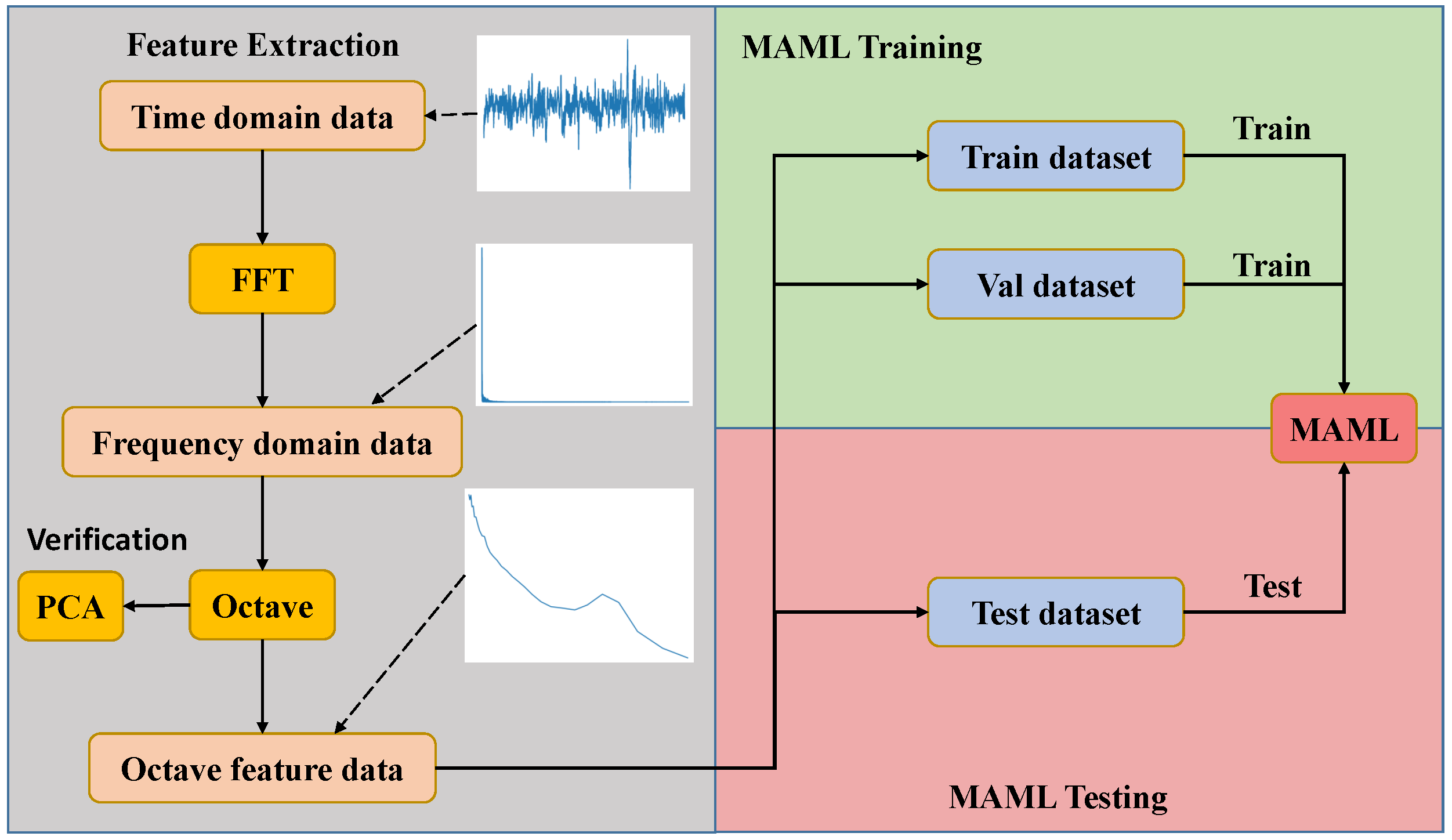
To achieve wind turbine blade defect detection with a small sample size, we developed an approach combining MAML and octave for defect detection. This approach is outlined in Figure 2:
(1)
We used fast Fourier transform (FFT) to convert the time-domain signal into the frequency domain;
(2)
We used the octave feature extraction algorithm to extract the features of the acoustic signals of wind turbine blades, then used principal component analysis (PCA) to analyze the spatial distribution of the samples;
(3)
We used the training set to train MAML-ANN, and used the validation set to adjust the training direction of the model;
(4)
We tested the performance of MAML-ANN using the test set, and compared its results with those of traditional ANN.

2.2. Octave Feature Extraction

For WTB signals, we could not analyze the frequency of each signal: this would be extremely time-consuming. So, we used the octave method to extract the feature information. Octave [24] is a macro signal analysis method that does not consider the amplitude of a specific frequency, but instead focuses on the power spectrum characteristics of the frequency band, which is composed of multiple frequencies. The steps for extracting the feature information using the octave method are as follows:
(1)
Divide the frequency bands according to the octave center frequency. The two methods to determine the octave center frequency are constant increase and constant percentage increase. In our method, we adopted the “GB3240-82 Preferred frequencies for the acoustic measurement” standard, which divides the discrete frequency domain into frequency bands with a constant bandwidth ratio. The reference frequency was 1000 Hz. The center frequency, lower cut-off frequency, and upper cut-off frequency of the frequency band can be expressed as:
f c e n t e r = 1000 × 10 n / 10 f l o w e r = f c e n t e r 2 N f u p p e r = 2 N f c e n t e r
where n represents an integer (0, ±1, ±2, ±3, ...); N is the order of the octave (1, 1/2, 1/3, 1/6, 1/12, 1/24, ...).
(2)
Calculate the sound pressure (SP) of each frequency band. The square sum of frequency points was used for each frequency band to obtain the SP, which can be expressed as:
P i = j = f l f u F j 2
where P i is the SP of the frequency band, f l is the lower cut-off frequency, f u is the upper cut-off frequency, and F j is the amplitude of the frequency point.
(3)
Calculate the sound pressure level (SPL) of each SP. Due to the logarithmic relation between human ears and frequency, SP must be converted into SPL. SPL can be expressed as:
S i = 20 log 10 P i / P r e f
where P r e f = 2 × 10 5 Pa, and P i denotes the SP values.

2.3. Model-Agnostic Meta-Learning

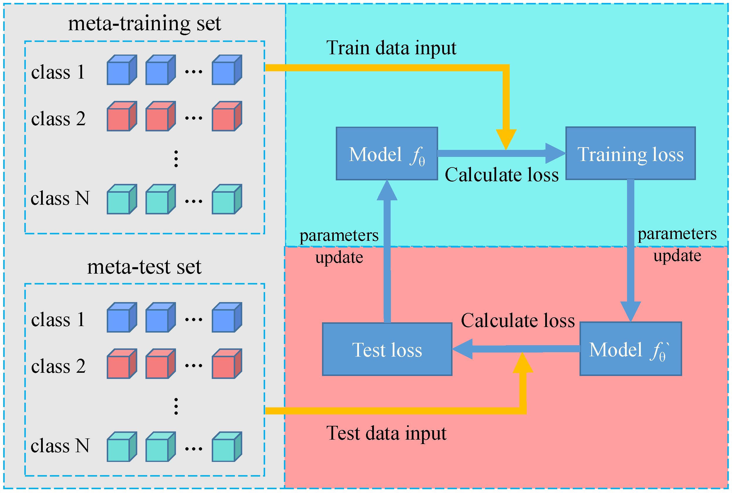
MAML [25] is an algorithm that trains the initial model parameters. The parameters of the model are explicitly trained such that a small number of gradient steps with a small amount of training data from a new task will produce good generalization performance on that task. Compared with the traditional model training, MAML adopts N-way K-shot and secondary gradient descent. It is more sensitive to changes in the task, such that small changes in the model parameters will produce substantial improvements on the loss function from all tasks from the training or testing data. The MAML training process is shown in Figure 3.
(1)
N-way K-shot
MAML training of the model parameters does not directly use data points, but rather a set of tasks. The task contains the meta-training set and meta-testing set. The meta-training set consists of K samples from each class, for a a total of N × K data points. The meta-testing set is composed of Q samples (q-shot) from each class (usually set to 2 or 5), for a total of N × Q data points.
(2)
Secondary gradient descent
For model training, the model is trained with the meta-training set to determine the training loss and obtain feedback from the corresponding loss, and is then tested on the meta-testing set to determine the testing loss. The model parameters are not optimized through training loss, but considering how the testing loss changes with respect to the parameters.
θ = θ α θ L m e t a t r a i n i n g f θ θ = θ β θ L m e t a t e s t f θ
where f denotes the model; L is the loss function; α and β are the learning rate of steps one and two, respectively; θ is the model parameters; θ is the updated model parameters.

2.4. Artificial Neural Network

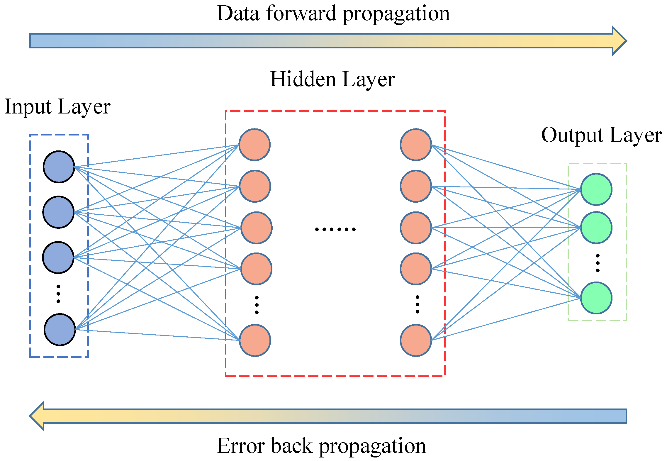
The artificial neural network [26] is a multilayer feedforward neural network trained according to the error reverse-propagation algorithm. It is usually composed of 3 parts: the input, hidden, and output layers. The output of each layer is directly sent to the next layer. The structure of the model is schematically presented in Figure 4.
The numbers of neurons in the input, hidden, and output layers are denoted by M, H i (where i is the number of the hidden layer), and N, respectively. The input data are X = x 1 , x 2 , , x M T , and the output of ANN is presented as Y = y 1 , y 2 , , y N T . The output of the nth neuron in the kth layer can be expressed as:
v n k = f m = 1 H k 1 w m n k v m k 1 + b n k
where H k 1 is the number of neurons in the previous hidden layer, w m n k is the weight from the mth neurons in the previous layer to the nth neuron in the current layer, v m k 1 is the output of the mth neuron in the previous layer, b n k is the offset parameter of the nth neuron in the current layer, f is the activation function (leaky ReLu was adapted in the ANN). The input data were fed to the input layer, and Y was generated by the output layer. Then, the neural network reversely transferred the error between the predicted and real values to adjust the parameters. The cross-entropy loss function was used to estimate the performance of ANN during the optimization process.

2.5. Evaluation Metrics

To address the binary classification problem of class imbalance, the confusion matrix is an effective evaluation method [27,28,29], which is defined in Figure 5. We defined the normal label as 0 and the abnormal label as 1 In the confusion matrix, true positive (TP) is defined as when the true label is 0 and the predicted label is also 0; false negative (FN) is defined as when the true label is 0 and the predicted label is 1; false positive (FP) is defined as when the true label is 1 and the predicted label is 0; and true negative (TN) is defined as when the true label is 1 and the predicted label is also 1. For WTB detection, we paid more attention to two indicators: precision and recall. They are a pair of contradictory measures. When the precision is high, the recall tends to be low, and vice versa. Estimating the merits and drawbacks of a model using precision and recall is difficult, so we introduced the F1 score. Using a confusion matrix, the above three evaluation indicators are defined by the following formulas, respectively:
Precision = T P T P + F P Recall = T P T P + F N F 1 = 2 × P × R P + R

2.6. Front-End Acoustic Acquisition System

To work normally in harsh environments, we used a specialized outdoor microphone unit DMK01, which was composed of a stainless steel body, a dedicated PR22 preamplifier, a noise cone, a specific windscreen, and a prepolarized weatherproof microphone 40CD. The unit was delivered with CUBE to realize data transmission and storage, as shown in Figure 6. The front-end acoustic acquisition system met the IEC61672 standard, which had a sampling frequency of 51.2 kHz, a large dynamic range (max to 118 dB), and its frequency response ranges from 20 Hz to 20 kHz. To ensure the reliability of the samples, we twice confirmed each acoustic signal. First, the status of wind turbine blades was investigated by professional institutions and wind farm staff before data acquisition. Second, the collected signals were identified and verified by the wind farm staff.

3. Results

3.1. Data Acquisition

To detect WTB defects, we went to two wind farms (Dawu and Diaoyutai) to collect the acoustic WTB signals. Selecting the location of the microphone in a harsh natural environment is difficult because the background noise can affect the analysis of the acoustic signals. In our experiment, we acquired the acoustic signals from different directions and heights, as shown in Table 1 and Figure 7. To verify the performance at different positions, we used the short-time Fourier algorithm to observe the defect information.
Because the collected acoustic signals contained a large amount of low-frequency wind noise, the defect information had low contrast on the time–frequency map. Therefore, we considered the time–frequency map above 1 kHz to facilitate the observation of the defect information. As shown in Figure 8, at the same height, the behind placement had the best ability to capture defects, front was second best, and the side placement was the worst. In the same direction, the ability to capture defects at different heights was similar because the microphones were directional. Therefore, the placement had a considerable influence on the signal-capturing ability of the microphone, whereas height had no influence. So, we decided to acquire signals at location B.

3.2. Acoustic Feature Extraction

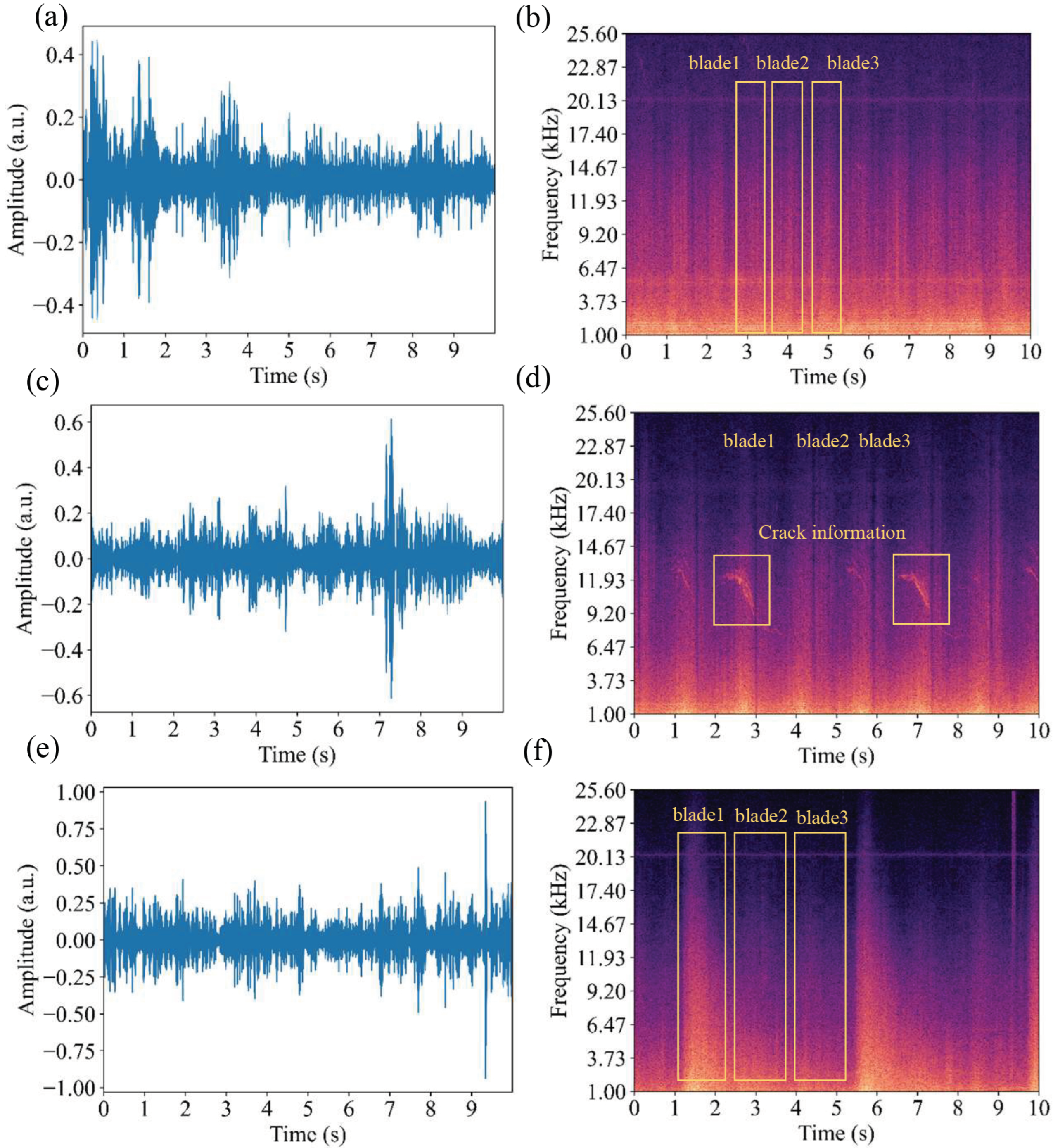
Next, we analyzed three different types of WTB acoustic signals to to achieve WTB defect detection, including the detection of normal status, cracks, and imbalance. The original acoustic signals and spectrograms of the different types are shown in Figure 9. As the acoustic signals show no notable characteristics, the different types of defects could not be distinguished in the time domain. Hence, we analyzed the acoustic signals of the different types using spectrograms. For normal signals, the spectrogram of each blade is the same as the other two. Compared with the normal signals, periodic crack information occurs in the spectrogram of crack signals, as shown in the yellow box in Figure 9d, which is due to cracks in the WTB. The unbalanced WTB signals also indicate a defect. A spectrogram of unbalanced signals is presented in Figure 9f, where the spectrogram of blade 1 is stronger than that of the other two.
As the acoustic signals showed no remarkable characteristics, we could not distinguish the different types of defects in the time domain. Hence, we used octave to extract defect information from the frequency domain. The order in the octave feature extraction algorithm must be carefully selected. The common orders are 1/3, 1/6, 1/12, 1/24, and so on. Different orders have different spectral resolutions, and their ability to describe spectral changes is different. In our experiment, we tried three orders, 1/3, 1/6, and 1/12, and discussed the performance of feature extraction and WTB defect detection of the different orders. As shown in Figure 10, the 1/3-octave features were sparse over the whole frequency. Within the defect frequency range of 10 kHz∼12.5 kHz, the interval of the frequency bands was too large to effectively extract the frequency change in the defect information. The characteristics of the 1/6 octave were relatively uniform over the whole spectrum, and the defect information was effectively extracted (capture the law of defect changes). Although the characteristics of the 1/12 octave could effectively obtain the defect information in the acoustic signal, the features were dense in the spectrum. This not only led to the complexity in the follow-up model but was also sensitive to changes in the natural environment. Finally, we selected 1/6 as octave order.
We analyzed the acoustic signals of different types of defects with the 1/6 octave, as shown in Figure 11. The 1/6-octave characteristics of the normal acoustic signals were similar to a power function. Compared with the normal signals, we observed an apparent protrusion in the crack signals at a specific frequency band (10∼12.5 kHz). For unbalanced signals, the octave features showed no obvious defect information, such as protrusion, but the characteristic octave curve was different, similar to a linear function. Therefore, the octave used in this study could effectively extract information regarding WTB defects, which is convenient for subsequent model training.
However, in the early stages of WTB damage, distinguishing defect information is challenging. This poses challenges for the detection of WTB defects: the traditional defect detection methods are unable to cope with this complex situation. For data visualization, we adopted PCA to reduce the feature dimensions from 31 to 3, preserving 84.5% of the feature information. As shown in Figure 12, most of the normal and abnormal samples could be effectively separated, but the boundary between classes was complex. With the rapid development of the new generation of artificial intelligence, ANN has provided opportunities to create new approaches to achieve defect detection. Nevertheless, the traditional ANN can be extremely easily overfit with complex boundaries and imbalanced classes. Therefore, we used MAML to solve the problem of small sample size and class imbalance to fit these complex boundaries.

3.3. Hyperparameter Selection

We obtained a large amount of data to verify the effectiveness of MAML-ANN. We collected a total of 2705 samples for the normal, crack, and unbalanced states, and the time length of each sample was 10 s. We divided all data into three parts, which were a training set (normal, 300 samples; abnormal, 300 samples), a validation set (normal, 51; abnormal, 199), and a testing set (normal, 264; abnormal, 1591). The percentages of normal, crack, and unbalance samples in dataset were 22.7%, 62.2%, and 15.1%, respectively. The shallow MAML-ANN we used in this experiment consisted of an input layer, three hidden layers, and an output layer, for which the number of neurons was M, (256, 128, 64), and 2, respectively. M was determined by the number of input data points. The hidden layer contained three layers, with 256, 128, and 64 neurons. The two was determined by the number of classes (normal and abnormal).
The selection of hyperparameters strongly impacted the performance of MAML-ANN. We analyzed the k-shot, q-shot, and batch size in this experiment. As shown in Figure 13, we discussed the performance of the model under different k-shot, q-shot, and batch size values. We considered 50 as an inflection point. When we had fewer than 50 data, MAML-ANN could not effectively distinguish samples from the different classes because the data size was too small. However, the accuracy rapidly increased as the data size increased. When the data size was greater than 50, the performance of the MAML-ANN can be slightly improved with the number of samples increasing. We verified that the training method could quickly learn the correlation function of each class of feature data in the case of small sample. By comparing and analyzing the effects of different hyperparameters, we found that changes in k-shot had no effect. The accuracy with a q-shot of two first increased and then decreased. When the q-shot was five, the accuracy was 2% higher on average than with a q-shot of two. The fluctuations in accuracy were 1.96% and 0.75% with q-shots of two and five, respectively. The latter was 38.3% of the former. In addition, when the batch size was four or eight, the accuracy was about 3.5% higher than when the batch size was two.
Considering the running time and other factors, we set the k-shot of the tasks to two, q-shot to five, batch size to four, and the learning rate to 0.0005, as shown in Table 2. To prevent overfitting in the training process, we added a dropout layer.

3.4. Performance of MAML-ANN

(1)
Comparison between MAML-ANN and traditional ANN
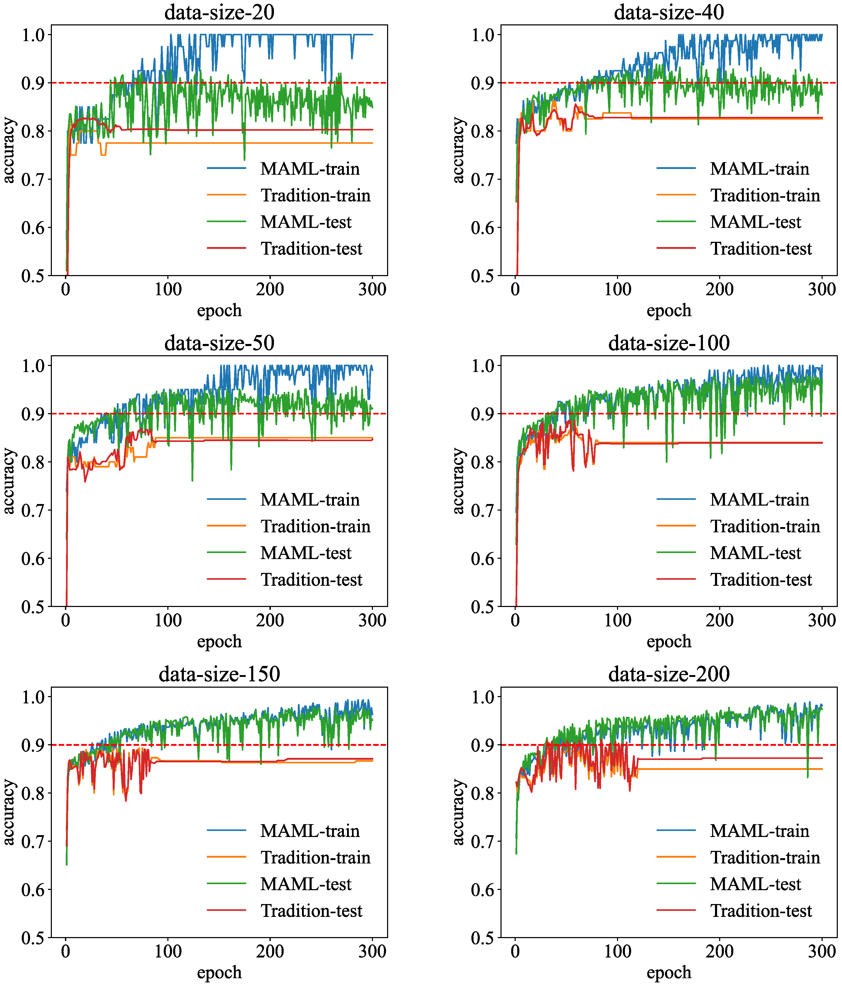
The performance evolution as a function of training iteration of MAML-ANN and traditional ANN is illustrated in Figure 14. In Figure 15, the results of MAML-ANN and traditional ANN are thoroughly analyzed for different data sizes. In general, the performance of MAML-ANN was better than that of traditional ANN. For traditional ANN, the accuracy slowly increased with the growth in data size. Overfitting occurred during the training process, and reached a stable state at around 100 epochs, indicating traditional ANN had fallen into a local optimum. Additionally, the average interval of accuracy for the normal and abnormal observations for different data sizes was higher than that of MAML-ANN, by about twice. This means that the model trended to one of the classes. The convergence of MAML-ANN was faster than that of traditional ANN, to produce a better model. Because the task was random, the accuracy showed certain volatility during the training process, which helped the model avoid the local optimum and find the global optimum. Moreover, this randomness caused the performance of the model to sharply deteriorate, but MAML-ANN could quickly adjust to a new and better solution. Overfitting also occurred in MAML-ANN. With the increase in epochs, the accuracy on the training and testing sets diverged. In addition, the overfitting gradually disappeared with the increase in data size, indicating MAML-ANN is still useful for large amounts of data. In summary, MAML-ANN produced a huge improvement of about 10% compared with traditional ANN. It not only has accurate performance when the sample size is small, but also showed good generalization performance with large amounts of data, and does not suffer from the problem of the training process falling into the local optimal solution.
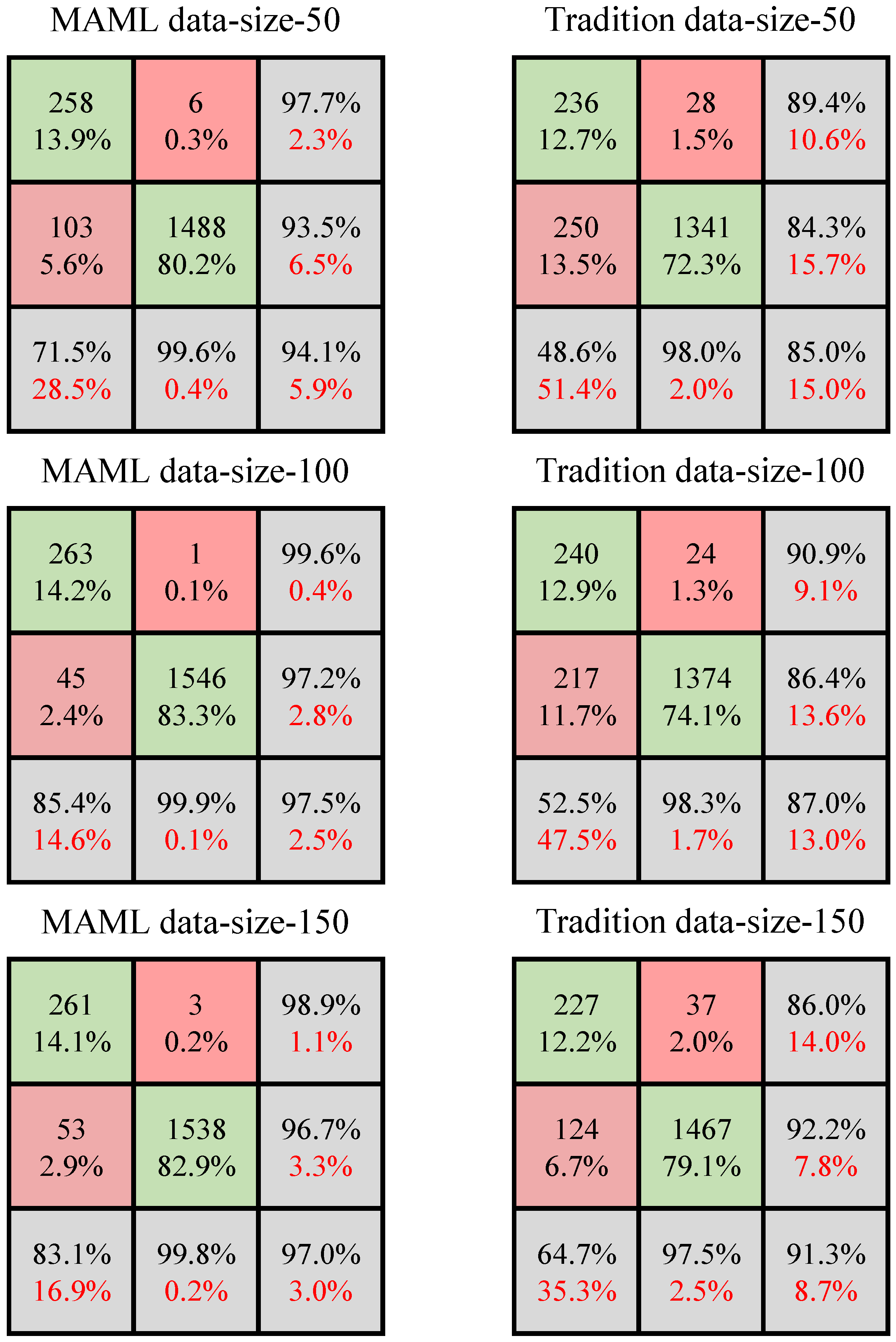
Figure 16 and Figure 17 show the confusion matrix and F1 score of MAML-ANN and traditional ANN for different data sizes. The TP and TN of MAML-ANN were both higher than those of traditional ANN for the same data size. The precision was approximately 10% higher, indicating the performance of MAML-ANN was better than that of traditional ANN. The recall was approximately 20% higher, which means the confidence in the predicted label was strong.
(2)
Recognition speed
To successfully apply MAML-ANN to a wind turbine blade defect monitoring system, the running time must meet the system requirements. The monitoring time interval of the wind turbine blade defect detection system is 5 min, and the signal acquisition time is 1 min. Therefore, the time from feature extraction to model judgment output results is less than 4 min. According to the test, the defect detection algorithm requires approximately 0.7 s for a 10 s signal, so it takes approximately 4.2 s for a 1 min signal, which is far less than the requirements of the system. It can be embedded into a wind turbine blade defect monitoring system.

4. Discussion

Our study has several limitations, especially the diversity of dataset. The types and degrees of WTB defects are diverse, but constructing a complete dataset is challenging. The dataset we constructed mainly contained normal, cracked, and unbalanced samples, but did not contain lightning strikes. This will result in poor performance for samples not included in the database. However, our method involved training the initial model parameters such that the model had maximal performance on new defects after a few gradient steps with a small amount of data. Furthermore, our proposed method is scalable. For wind turbine blade defect detection, the single-modal defect detection method can only detect some defects well, but cannot detect all defects. The use of multimodal defect detection, such as acoustics, vision, infrared, etc., is the future development trend. Our proposed scheme can be well-integrated with other detection schemes to achieve multimodal defect detection.

5. Conclusions

In our study, we designed and experimentally tested an acoustic detection method based on MAML. The results showed that the proposed method can very accurately detect defects in WTBs. To verify our method, we collected signals from WTBs on wind farms and discussed the impact of different directions and heights of sensor placement on data acquisition. We explored the performance of feature extraction in different octaves, from which we selected the 1/6 octave. Finally, we analyzed the characteristics of the three defect types (normal, crack, and imbalance) in detail and verified the performance of MAML-ANN. Compared with traditional ANN, MAML-ANN performed better and achieving a defect detection accuracy of 94.1% when the sample size was only 50. Moreover, MAML-ANN has a fast convergence speed and can automatically search for the global optimal solution. The method also performed well with a larger data sample, indicating the MAML-ANN is suitable for small as well as large sample sizes. Our proposed method offers an attractive option to improve the detection of WTB defects from small sample sizes, and reduces the labor cost for WTB data collection.
In the future, we will study the defect detection method for wind turbine blades from two aspects: first, we want to obtain acoustic signals through artificially produce damage. Second, we want to try tree-based algorithms [30] for WTB defect detection.

Author Contributions

Data curation, Y.Z., Y.W., S.L. and Q.C.; formal analysis Y.Z.; methodology, Y.Z.; project administration, X.L. All authors have read and agreed to the published version of the manuscript.

Funding

This study was supported by Shenzhen Science and Technology Programe (No. GJHZ20210705142538004).

Institutional Review Board Statement

Not applicable.

Informed Consent Statement

Not applicable.

Data Availability Statement

Not applicable.

Conflicts of Interest

The authors declare no conflict of interest.

References

  1. De Azevedo, H.D.M.; Araújo, A.M.; Bouchonneau, N. A review of wind turbine bearing condition monitoring: State of the art and challenges. Renew. Sustain. Energy Rev. 2016, 56, 368–379. [Google Scholar] [CrossRef]
  2. Tummala, A.; Velamati, R.K.; Sinha, D.K.; Indraja, V.; Krishna, V.H. A review on small scale wind turbines. Renew. Sustain. Energy Rev. 2016, 56, 1351–1371. [Google Scholar] [CrossRef]
  3. Chen, X.; Yan, R.; Liu, Y. Wind turbine condition monitoring and fault diagnosis in China. IEEE Instrum. Meas. Mag. 2016, 19, 22–28. [Google Scholar] [CrossRef]
  4. Lau, B.C.P.; Ma, E.W.M.; Pecht, M. Review of offshore wind turbine failures and fault prognostic methods. In Proceedings of the IEEE 2012 Prognostics and System Health Management Conference (PHM-2012 Beijing), Beijing, China, 23–25 May 2012; pp. 1–5. [Google Scholar]
  5. Liu, W.Y.; Tang, B.P.; Han, J.G.; Lu, X.N.; Hu, N.N.; He, Z.Z. The structure healthy condition monitoring and fault diagnosis methods in wind turbines: A review. Renew. Sustain. Energy Rev. 2015, 44, 466–472. [Google Scholar] [CrossRef]
  6. Matsui, T.; Yamamoto, K.; Ogata, J. Study on improvement of lightning damage detection model for wind turbine blade. Machines 2021, 10, 9. [Google Scholar] [CrossRef]
  7. Chen, B.; Zhang, M.; Lin, Z.; Xu, H. Acoustic-based whistle detection of drain hole for wind turbine blade. ISA Trans. 2022; in press. [Google Scholar] [CrossRef]
  8. Du, Y.; Zhou, S.; Jing, X.; Peng, Y.; Wu, H.; Kwok, N. Damage detection techniques for wind turbine blades: A review. Mech. Syst. Signal Process. 2020, 141, 106445. [Google Scholar] [CrossRef]
  9. Zhang, C.; Yang, T.; Yang, J. Image recognition of wind turbine blade defects using attention-based MobileNetv1-YOLOv4 and transfer learning. Sensors 2022, 22, 6009. [Google Scholar] [CrossRef]
  10. Zhang, Y.; Avallone, F.; Watson, S. Wind turbine blade trailing edge crack detection based on airfoil aerodynamic noise: An experimental study. Appl. Acoust. 2022, 191, 108668. [Google Scholar] [CrossRef]
  11. Wang, L.; Zhang, Z. Automatic detection of wind turbine blade surface cracks based on UAV-taken images. IEEE Trans. Ind. Electron. 2017, 64, 7293–7303. [Google Scholar] [CrossRef]
  12. Yang, K.; Rongong, J.A.; Worden, K. Damage detection in a laboratory wind turbine blade using techniques of ultrasonic NDT and SHM. Strain 2018, 54, e12290. [Google Scholar] [CrossRef]
  13. Naderi, E.; Khorasani, K. Data-driven fault detection, isolation and estimation of aircraft gas turbine engine actuator and sensors. Mech. Syst. Signal Process. 2018, 100, 415–438. [Google Scholar] [CrossRef]
  14. Jiang, S.; Lin, P.; Chen, Y.; Tian, C.; Li, Y. Mixed-signal extraction and recognition of wind turbine blade multiple-area damage based on improved Fast-ICA. Optik 2018, 179, 1152–1159. [Google Scholar] [CrossRef]
  15. Su, Y.; Meng, L.; Kong, X.; Xu, T.; Lan, X.; Li, Y. Small sample fault diagnosis method for wind turbine gearbox based on optimized generative adversarial networks. Eng. Fail. Anal. 2022, 140, 106573. [Google Scholar] [CrossRef]
  16. Liu, J.; Qu, F.; Hong, X.; Zhang, H. A small-sample wind turbine fault detection method with synthetic fault data using generative adversarial nets. IEEE Trans. Ind. Inform. 2019, 15, 3877–3888. [Google Scholar] [CrossRef]
  17. Guo, Y.; Zhong, L.; Qiu, Y.; Wang, H.; Gao, F.; Wen, Z.; Zhan, C. Using ISU-GAN for unsupervised small sample defect detection. Sci. Rep. 2022, 12, 11604. [Google Scholar] [CrossRef]
  18. Hassani, S.; Mousavi, M.; Gandomi, A.H. Structural health monitoring in composite structures: A comprehensive review. Sensors 2021, 22, 153. [Google Scholar] [CrossRef] [PubMed]
  19. Teng, W.; Ding, X.; Tang, S.; Xu, J.; Shi, B.; Liu, Y. Vibration analysis for fault detection of wind turbine drivetrains—A comprehensive investigation. Sensors 2021, 21, 1686. [Google Scholar] [CrossRef]
  20. Antoniadou, I.; Dervilis, N.; Papatheou, E.; Maguire, A.E.; Worden, K. Aspects of structural health and condition monitoring of offshore wind turbines. Philos. Trans. A Math. Phys. Eng. Sci. 2015, 373, 20140075. [Google Scholar] [CrossRef] [Green Version]
  21. Tsai, T.C.; Wang, C.N. Acoustic-based method for identifying surface damage to wind turbine blades by using a convolutional neural network. Meas. Sci. Technol. 2022, 33, 085601. [Google Scholar] [CrossRef]
  22. Patange, A.D.; Jegadeeshwaran, R.; Bajaj, N.S.; Khairnar, A.N.; Gavade, N.A. Application of machine learning for tool condition monitoring in turning. Sound Vibrat. 2022, 56, 127–145. [Google Scholar] [CrossRef]
  23. Jatakar, K.H.; Mulgund, G.; Patange, A.D.; Deshmukh, B.B.; Rambhad, K.S. Multi-point face milling tool condition monitoring through vibration spectrogram and LSTM-autoencoder. Int. J. Perform. Eng. 2022, 18, 570. [Google Scholar] [CrossRef]
  24. Zhang, Y.; Cui, Y.; Xue, Y.; Liu, Y. Modeling and measurement study for wind turbine blade trailing edge cracking acoustical detection. IEEE Access 2020, 8, 105094–105103. [Google Scholar] [CrossRef]
  25. Finn, C.; Abbeel, P.; Levine, S. Model-agnostic meta-learning for fast adaptation of deep networks. In Proceedings of the 34th International Conference on Machine Learning (ICML 2017), Sydney, Australia, 6–11 August 2017; Volume 70, pp. 1126–1135. [Google Scholar]
  26. Goodfellow, I.; Bengio, Y.; Courville, A. Deep Learning; MIT Press: London, UK, 2016. [Google Scholar]
  27. Janeliukstis, R. Continuous wavelet transform-based method for enhancing estimation of wind turbine blade natural frequencies and damping for machine learning purposes. Measurement 2021, 172, 108897. [Google Scholar] [CrossRef]
  28. Tong, R.; Li, P.; Lang, X.; Liang, J.; Cao, M. A novel adaptive weighted kernel extreme learning machine algorithm and its application in wind turbine blade icing fault detection. Measurement 2021, 185, 110009. [Google Scholar] [CrossRef]
  29. Zhou, Z.H. Machine Learning, 1st ed.; Springer: Singapore, 2021. [Google Scholar]
  30. Deo, T.Y.; Patange, A.D.; Pardeshi, S.S.; Jegadeeshwaran, R.; Khairnar, A.N.; Khade, H.S. A white-box SVM framework and its swarm-based optimization for supervision of toothed milling cutter through characterization of spindle vibrations. arXiv 2021, arXiv:2112.08421. [Google Scholar]
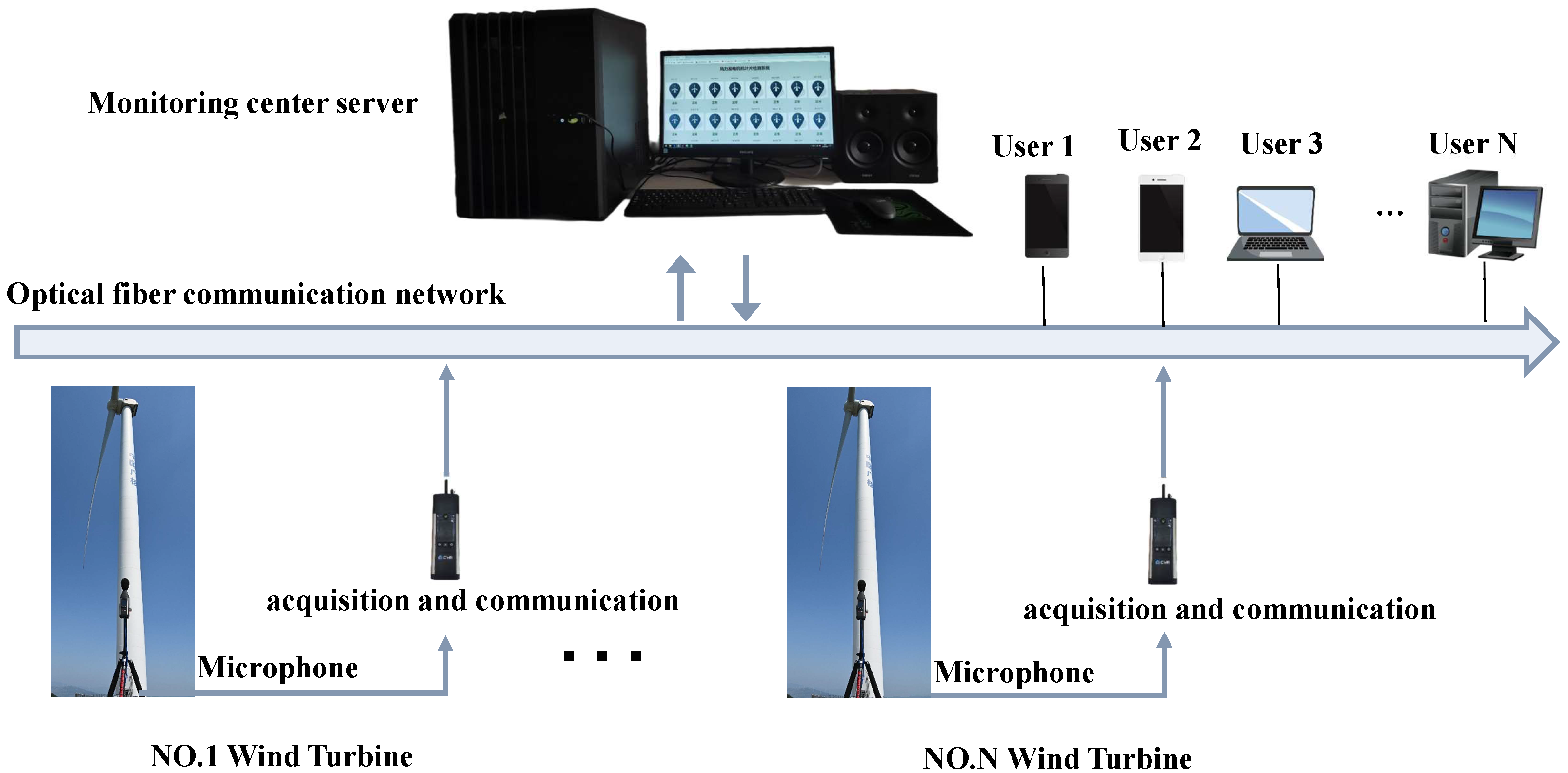
Figure 1. Wind turbine blade defect detection system.
Machines 10 01184 g001
Figure 2. Workflow of the MAML-based acoustic defect detection approach.
Machines 10 01184 g002
Figure 3. Diagram of MAML.
Machines 10 01184 g003
Figure 4. Schematic diagram of ANN structure.
Machines 10 01184 g004
Figure 5. Schematic of the confusion matrix.
Machines 10 01184 g005
Figure 6. Front-end acoustic acquisition system.
Machines 10 01184 g006
Figure 7. Data acquisition at wind farm: (a) location C; (b) location D.
Machines 10 01184 g007
Figure 8. Time–frequency map at different locations: (a) A; (b) B; (c) C; (d) D; (e) E; (f) F.
Machines 10 01184 g008
Figure 9. Time domain and spectrogram of different signals: (a) time domain and (b) spectrogram of normal signal; (c) time domain and (d) spectrogram of crack signal; (e) time domain; and (f) spectrogram of unbalanced signal.
Machines 10 01184 g009
Figure 10. Octave performance with different orders for cracked WTB signal.
Machines 10 01184 g010
Figure 11. The 1/6-octave feature of different types of defects.
Machines 10 01184 g011
Figure 12. Visualization of data (red: normal, blue: abnormal).
Machines 10 01184 g012
Figure 13. Comparison between accuracies for different (a) k-shot, (b) q-shot, and (c) batch size.
Machines 10 01184 g013
Figure 14. Training process of MAML-ANN and traditional ANN.
Machines 10 01184 g014
Figure 15. Performance of MAML-ANN and traditional ANN. (a) Accuracy for different data sizes; (b) average interval of accuracy between normal and abnormal samples.
Machines 10 01184 g015
Figure 16. F1 score of MAML-ANN and traditional ANN.
Machines 10 01184 g016
Figure 17. Confusion matrix of MAML-ANN and traditional ANN for different data sizes.
Machines 10 01184 g017aMachines 10 01184 g017b
Table 1. Locations with different placements and heights.
LocationPlacementHeight (m)
Abehind5
Bbehind1.5
Cfront5
Dfront1.5
Eside5
Fside1.5
Table 2. Hyperparameters of MAML-ANN.
HyperparametersNumerical
learning rate0.0005
k-shot2
q-shot5
batch size4
Publisher’s Note: MDPI stays neutral with regard to jurisdictional claims in published maps and institutional affiliations.