Design and Implementation of Simulation-Based Scheduling System with Reinforcement Learning for Re-Entrant Production Lines

Abstract

Recently, manufacturing companies have been making efforts to increase resource utilization while ensuring the flexibility of production lines to respond to rapidly changing market environments and customer demand. In the high-tech manufacturing industry, which requires expensive manufacturing facilities and is capital-intensive, re-entrant production lines are used for efficient production with limited resources. In such a production system, a part visits a specific station repeatedly during the production period. However, a re-entrant production line requires an appropriate scheduling system because other parts with different processing requirements are processed at the same station. In this study, a re-entrant production line was modeled as a manufacturing environment via simulation, and an adaptive scheduling system was developed to improve its operational performance by applying deep reinforcement learning (DRL). To achieve this, a software architecture for integrating DRL with the simulation was developed and the states, actions, and rewards of the reinforcement learning (RL) agent were defined. Moreover, a discrete-event simulation control module was designed to collect data from the simulation model and evaluate the policy network trained via DRL. Finally, the applicability and effectiveness of the developed scheduling system were verified by conducting experiments on a hypothetical re-entrant production line.

1. Introduction

Responding to rapidly changing market environments and customer demands is becoming increasingly important [1,2,3]. In particular, optimal production line operation is required to increase the variety of products, owing to the transition of product production systems from small-quantity batch production to personalized production [4]. Therefore, manufacturing companies are making efforts to increase productivity while ensuring the flexibility of their production lines [5,6].

In particular, in high-tech manufacturing industries such as those producing semiconductors, liquid crystal displays, and printed circuit boards, which require expensive manufacturing facilities and are capital-intensive, re-entrant production lines are used to achieve efficient production with limited resources [7,8,9]. Although all industries do not have the same levels of requirements for re-entrant production lines, some manufacturing companies have already adopted highly flexible production lines. For example, major companies in the automotive industry such as Tesla, Volkswagen, and General Motors have replaced traditional conveyor systems with automated guided vehicle (AGV) systems in some electric battery vehicle production lines. This demonstrates their aim to utilize re-routing-capable and highly flexible production lines that can be reconfigured to re-entrant production lines. The defining characteristic of a re-entrant production line is that a single job visits a specific station more than once during the processing period, including cases where rework is required owing to quality problems [10]. However, in a re-entrant production line, various parts with different processing requirements need to be processed at the same station and predicting the arrival of a product is difficult [11]. Conventionally, re-entry production systems on actual shop floors are operated using a single priority-based dispatching rule, owing to the complexity of a re-entrant production line [12,13].

Although most existing manufacturing systems, including re-entrant production lines, operate at near-optimal productivity under steady conditions, maintaining optimal productivity in an actual production environment is generally difficult because of unpredictable conditions. Example conditions are new orders, demand volume changes, re-scheduling, and station failures. These unpredictable conditions account for a decrease of 80% in the overall station efficiency and a loss of 50% in resource utilization [14,15]. Thus, if a dynamic manufacturing environment relies solely on a single priority-based dispatching rule, adequate responses to dynamic conditions are impossible and productivity is likely to decrease. Specifically, an adaptive scheduling system is required to respond to unexpected events in a timely manner and implement a complex system such as a re-entrant production line. It maximizes productivity by reducing the time and cost requirements related to unexpected events and increases overall resource utilization [16].

One simple example of a re-entrant production line is a job that is re-added to the production line for quality retreatment. Specifically, if there are m machines and n jobs, such a re-entrant production line processes the n jobs more than once in one machine. Two types of re-entrant production lines were extensively studied: re-entrant flow shops (RFSs) and re-entrant job shops (RJSs). The difference between RFSs and RJSs is related to the operation sequence in the aforementioned premise. A shop is defined as an RFS when a part is produced as a finished product in a certain sequence using all machines, whereas it is defined as an RJS when a finished product is produced by different sequences for all jobs. The conceptual diagram of a re-entrant production line is shown in Figure 1 [17].

Studies have attempted to solve various types of re-entrant production line scheduling problems using mathematical, heuristic, and metaheuristic techniques. Narahari and Khan [18] (1996) used margin valuation adjustment (MVA) to compare the performance of priority-based dispatching rules in operating a re-entrant production line. Park et al. [19] (2002) analyzed the performance of MVA in a re-entrant production line composed of single-task and multipurpose machines and compared it to those of various priority-based dispatching rules. Choi and Ko [20] (2009) solved the problem of late deliveries using branches and bounds in a re-entrant production line with two facilities and evaluated the system performance via simulation. However, traditional mathematical modeling techniques cannot model the large and complex production lines of actual manufacturing environments while reflecting their dynamic characteristics.

Chen et al. [12] (2004) proposed a dynamic state-dependent dispatching (DSDD) heuristic method and applied it based on the state of the re-entrant production line by combining and modifying the conventional dispatching rules. In their study, six single dispatching rules were compared with the proposed DSDD by selecting lead time as the performance index. Zhang et al. [13] (2009) applied the dispatching rules to bottleneck processes by proposing a dynamic bottleneck dispatching policy that integrates simulation and response surface methodology. Although heuristic dispatching rules are easy to implement in a complex re-entrant production line, their application to an actual production line remains difficult because experiments are conducted on a simple model that does not consider unexpected events of production.

Furthermore, several metaheuristic approaches were proposed. Rifai et al. [21] (2016) proposed an improved genetic algorithm to solve the re-entrant flexible manufacturing system (FMS) scheduling problem. The makespan, average flow time, and delay were reduced by determining the optimal operation sequence and route using the proposed methodology. Chen et al. [22] (2008) solved the re-entrant flow process problem without job priority by applying hybrid tabu search (HTS). Nawaz et al. [23] (1983) solved the scheduling problem of a re-entrant production line using HTS and compared its solution with those of integer programming and general tabu search by dividing the problem by size. Jain et al. [24] (2003) performed simulated annealing of the scheduling problem of a re-entrant wafer-manufacturing process and compared its solution with those of the conventional dispatching rules based on the average cycle time and job delay.

Many studies using mathematical, heuristic, and metaheuristic techniques have attempted to solve the re-entrant production line scheduling problem. However, none were able to model the complexity and dynamic characteristics of real-world problems while ensuring a short computation time.

Recently, the use of reinforcement learning (RL) for scheduling has been gaining prominence because of the demonstrated ability of RL to achieve a short computation time and address complex optimization problems. RL is a machine-learning-based approach that involves defining a policy as a series of actions in which one or multiple agents explore an environment, identify the current state, and maximize the accumulation of rewards. A reward is a scalar feedback signal that indicates the performance of an agent in each state of the environment, using which the success of its action is evaluated. An agent is trained to maximize the total sum of the rewards because such interactions are repeated [25]. The Markov decision process (MDP) is used as an environment for RL. The MDP involves a series of processes in which the concepts of rewards and actions are added to the probabilistic state-changing process as time progresses [26].

In tabular RL methods, agents are trained by storing and updating values of all states in the form of a table in an environment represented by the MDP. However, this method has limitations in representation as it requires a longer time to learn when the problem becomes larger and more complex. Deep RL (DRL) was developed to solve this problem. While RL considers the problem of agents learning and making decisions by trial and error, DRL incorporates deep learning into the solution, allowing agents to make decisions from unstructured input data and approximate the state values as nonlinear functions using a deep neural network, which can efficiently learn an environment of any type or size [27]. Once a DRL model is trained, it can take the optimal action at each decision-making point and respond to dynamic scenarios in real-time. In the manufacturing field, as the design and operation of manufacturing systems and production lines become more complex, a faster and more accurate decision-making system is required. Such improved performance and features make it possible to apply DRL in various ways in the manufacturing field [27,28,29,30,31,32].

A deep Q-network (DQN) is a value-function-based DRL algorithm. Waschneck et al. [28] (2018) trained multiple agents to select the optimal dispatching rule using a DQN to maximize rewards in a shop. Shiue et al. [29] (2018) solved a DRL-based real-time scheduling problem to respond to changes in a dynamic shop environment. Hu et al. [30] (2020) applied DQN to the scheduling problem of an FMS modeled by Petri net and confirmed the effectiveness of DRL compared with a heuristic method. Luo [14] (2020) used the double DQN (DDQN) algorithm to respond to a continuous production state and select the most suitable dispatching rule at the time of schedule change. Stricker et al. [31] (2018) applied a DQN to manufacturing systems in the semiconductor industry. However, most previous studies using DRL have a common limitation—they used deterministic mathematical models to model the learning environment. Wang and Chatwin [32] (2005) identified the following problems that arise when using deterministic mathematical approaches for modeling complex manufacturing systems:

• Mathematical models may be impractical because the probabilistic elements of complex manufacturing systems cannot be expressed accurately;
• Mathematical models may be invalid because theoretical modeling of complex dynamic systems requires excessive simplification;
• Mathematical models frequently generate unrealistic solutions in system optimization because they are based on oversimplified assumptions.

Therefore, this study uses a manufacturing simulation tool to model a production line and a scheduling problem, thereby allowing a more realistic stochastic learning environment for RL than mathematical approaches. Thus, the objective of this study is to develop a DRL-integrated scheduling system and a training procedure that can improve the operational performance of a complex re-entrant production line modeled using a manufacturing simulation tool.

The remainder of this paper is organized as follows. In Section 2, the concept of a re-entrant production line is briefly introduced and the re-entrant production line scheduling problem is formalized. In Section 3, the software architecture for the manufacturing simulation, the DRL-integrated scheduling system and its training process are described. In addition, each component module in the proposed scheduling system is explained in detail. Section 4 discusses the experimental verification of the effectiveness of the proposed methodology. Finally, in Section 5, the conclusions of this study and the scope for future research are presented. Abbreviations summarizes the notations used in this paper.

2. Problem Definition

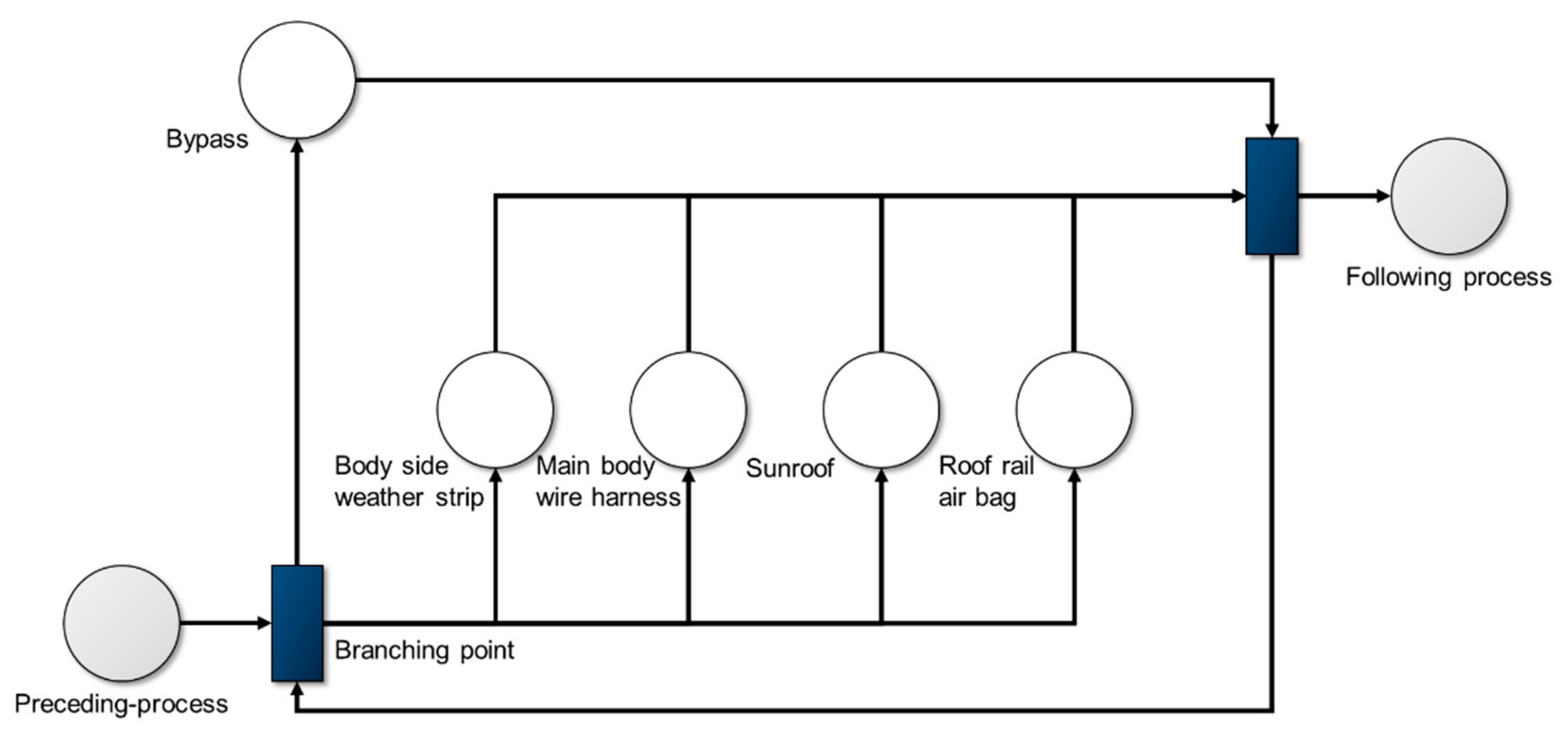
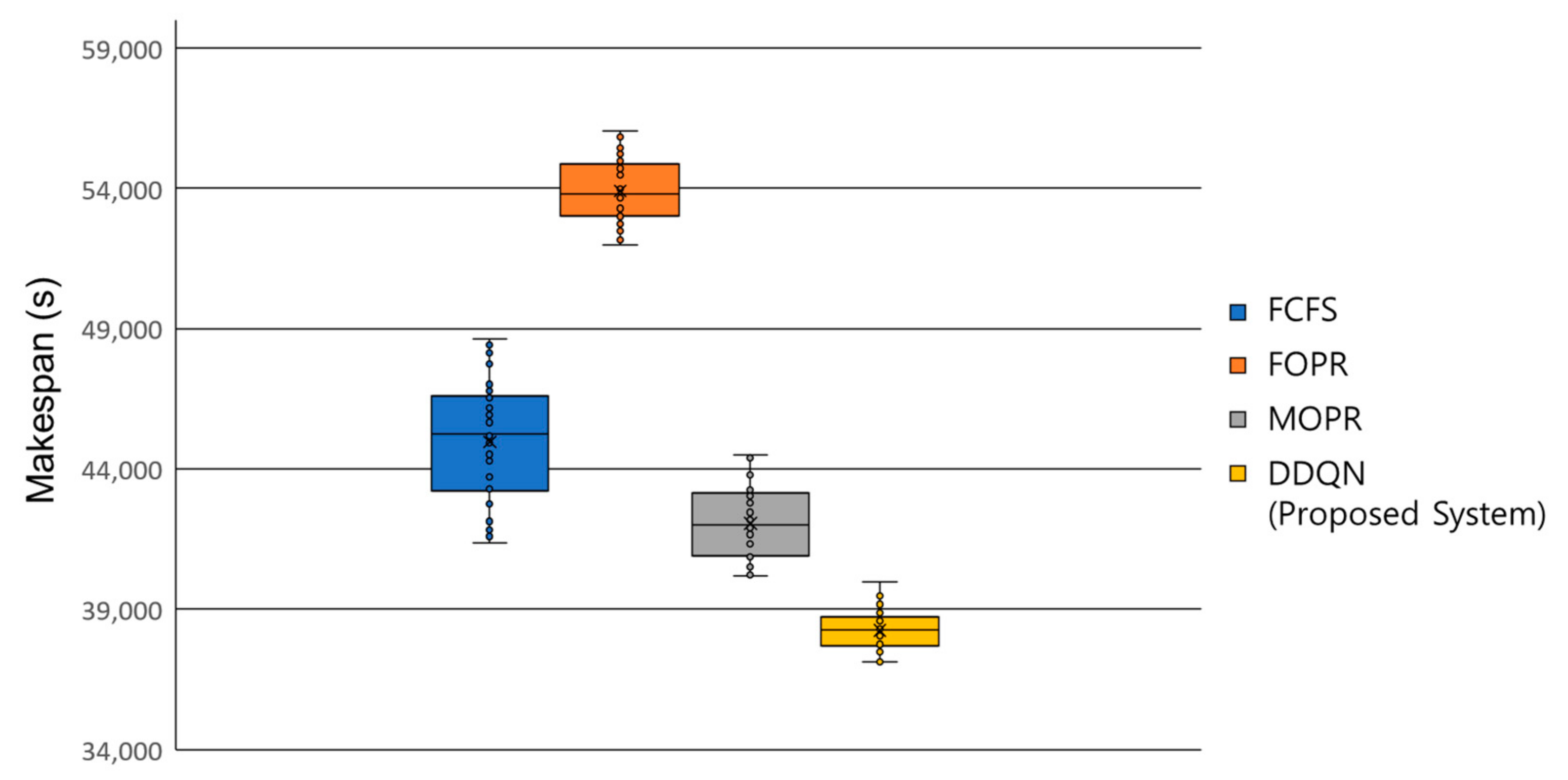
The scheduling problem considered in this study deals with a re-entrant production line. A schematic of the target re-entrant production line is shown in Figure 2. This re-entrant production line is a conceptual production system that focuses on an automobile assembly process in which a vehicle is assumed to be conveyed by a smart transporter, such as an AGV. It is composed of a process line, bypass line, and branching point. At the branching point, a decision is made to dispatch a vehicle in one direction between two competing lines: process and bypass lines. Vehicles coming from the preceding process line enter the re-entrant production line, in which they are assumed to have interchangeable job sequences, i.e., each job required to build a vehicle has no priority and is independent of the other jobs. The process line is composed of four assembly stations in parallel, and vehicles are processed at each station. For the dispatching of vehicles, three priority-based dispatching rules are considered. The first dispatching rule is first come, first served (FCFS), in which vehicles are processed in the order of arrival at the branching point. The second dispatching rule is the fewest number of operations remaining (FOPR), and it dispatches vehicles in the order of the least number of remaining operations. The third rule is the most number of operations remaining (MOPR), and it arranges vehicles in the order of the highest number of remaining operations.

The shown system operates as follows. The branching point prioritizes and branches out the vehicles coming from the preceding process or returning from the bypass line according to the dispatching rule. One branch is the process line and the other is the bypass line. If a vehicle is dispatched to enter the bypass line, it takes the bypass line and returns to the branching point after a full empty trip, following which the vehicle is dispatched again. However, if a vehicle is dispatched to the process line, it is assigned to one of the available stations. When all required processes are finished, the vehicle moves to the post-processing line. As described, the target re-entrant production system does not have a fixed in-line configuration, instead, it has the form of an RJS, in which inputs are dispatched to either the process or bypass line. Consequently, the re-entrant production line and its operation rules lead to a challenging issue: reliance on a single priority-based dispatching rule, which hampers the performance because of its myopic view and evaluation of only the current state. Therefore, this study establishes an adaptive DRL-based dispatching method by combining simple priority-based dispatching rules and choosing one rule as an action from a specific state such that the accumulation of rewards is maximized. It should be noted that this study uses makespan, denoted as $C_{max}$, as the performance measure. Therefore, the global cost function minimizes $C_{max}$, and the reward for an action of the RL agent is designed to be proportional to the goal of minimizing $C_{max}$, which is discussed in the next section.

3. Manufacturing Simulation and DRL-Integrated Scheduling System

In this section, a DRL-integrated scheduling system for manufacturing simulation is proposed. The re-entrant production line, which provides a learning environment, is modeled using a simulation tool. This study uses Siemens Plant Simulation 15.1 as the simulation modeling tool. In addition, it uses Python 3.7 with Pytorch and C# to implement the DRL modules and other classes for system module integration.

3.1. Manufacturing Simulation and DRL-Integrated Software Architecture

The proposed DRL-integrated software architecture is presented in Figure 3. It consists of an RL module, a simulation control module, and a discrete simulation model of the underlying manufacturing system (i.e., the re-entrant production line). The discrete simulation model is controlled by a discrete-event simulation (DES) control module, which is triggered by discrete events. From the overall system perspective, the RL module trains the agent using data received from the DES control module, updates the policy network, and transmits the policy network parameters back to the DES control module. The DES control module executes the simulation by reflecting the updated policy network in the simulation model and evaluates the transmitted policy network. Once the simulation is completed, the data required for training are collected and transmitted to the RL module again. This interaction cycle is repeated until the termination condition is satisfied, following which the RL module is finally trained to infer the optimal policy (i.e., the best dispatching rule) for each state of the manufacturing environment. Concurrently, because the RL module learns the optimal policy without formulating an MDP model explicitly, the proposed approach is classified as a model-free approach.

3.2. Training Process of DRL Using Manufacturing Simulation Tool

The proposed training process to apply DRL to the re-entrant production line is as follows.

Step 1: The re-entrant production line is modeled using the simulation tool and becomes a learning environment. The simulation model contains information about the product, process, plan, and resources of the manufacturing system. The information includes the bill of materials, work order, production volume, manufacturing processes, driving control parameters of the AGVs, and vehicle incoming sequences.

In addition, a deep neural network is constructed in the simulation model and continues to replace or upgrade its weight and bias data with the trained weights and bias data from the RL module in the training procedure. The deep neural network in the simulation model is a type of twin version of the policy network in the RL module. It selects actions (i.e., dispatching rules) to take for each state to advance the simulation step. Based on the throughput performance measured after one simulation run is completed, the performance of the trained policy network is evaluated. A separate table is constructed and used to update the learned weight and bias data in the deep neural network during the training process. This is shown in Figure 4.

Step 2: The state observed by the RL agent is defined as a vector variable that is sufficiently large to represent the current state of the production line without major information loss. The components of the state variable include the number of remaining parts per job that are added to the re-entrant production line and the number of works in process (WIPs) per process in the re-entrant production line. The data regarding the number of remaining parts per job are collected with the dimension equaling the number of jobs, and those regarding the number of WIPs per process in the production line are collected with the dimension equaling the number of processes. An action of the agent is defined by the selection of one dispatching rule among three candidate rules (i.e., FCFS, FOPR, and MOPR). The components of the state variable are summarized in

Table 1. Components of state.

Feature	Description	Dimension
Number of remaining parts per job	Number of parts to be produced for each job in the production plan	$N_j$
Number of WIPs by process	Number of reworks by process in the production line	$N_j$

.

Step 3: Makespan is used as the performance index of the target re-entrant production line. However, the re-entrant production line has a dynamic manufacturing environment, and thus, predicting the next state is uncertain. Therefore, fully understanding the effects of the dispatching rules selected by the RL agent based on the makespan measured after all vehicles are produced or one simulation run is completed is difficult. Moreover, the makespan can be obtained after a long time delay; therefore, it is inappropriate for use as an immediate reward for training the RL agent. Therefore, instead of using the makespan as it is, this study uses the production completion time of each vehicle to create an immediate reward for an action. In detail, the average of the production completion time intervals of vehicles for a certain period after a dispatching rule is selected is used as the reward. Specifically, the average production completion time interval is treated as a reward for each episode, and the conceptual diagram of the reward measurement according to the dispatching rule is shown in Figure 5. In the figure, $t$,$s$, $a$, and $r$ denote the time epoch corresponding to one episode, state, action (i.e., selection of the dispatching rule), and reward, respectively.

Consequently, the reward of selecting an action at the current state becomes available in the next state after a certain period denoted by $\rho$. For more clarity, the reward function, $r_i$, for calculating the average production completion time interval over a certain period is expressed in Equation (1). Note that in the formula, a minus sign is used to drive the RL agent to take an action to reduce the interval time. The relationship between $C_{max}$ and the immediate reward is expressed in Equation (2).

$$r_i=-\frac{1}{N_i^{\rho }}{\displaystyle \sum _{k=1}^K}\left({\mu }_{i_k}-{\mu }_{i_{k-1}}\right),i\ge 0,\left({\mu }_{i_0}=0\right)$$

(1)

$$C_{max}\propto \frac{1}{N_i^{\rho }}{\displaystyle \sum _{k=1}^K}\left({\mu }_{i_k}-{\mu }_{i_{k-1}}\right),i\ge 0$$

(2)

where ${\mu }_{i_k}$ denotes the production completion time of the $k$-th product in the $i$-th period and $N_i^{\rho }$ represents the number of products completely produced in the $i$-th period. Equation (2) suggests that the vehicle production interval time is proportional to $C_{max}$. Therefore, if the RL agent wants to earn a higher reward, it needs to take an action that reduces the interval time in accordance with the global cost function, which aims to minimize $C_{max}$. The definitions of the other notations are presented in Table 1.

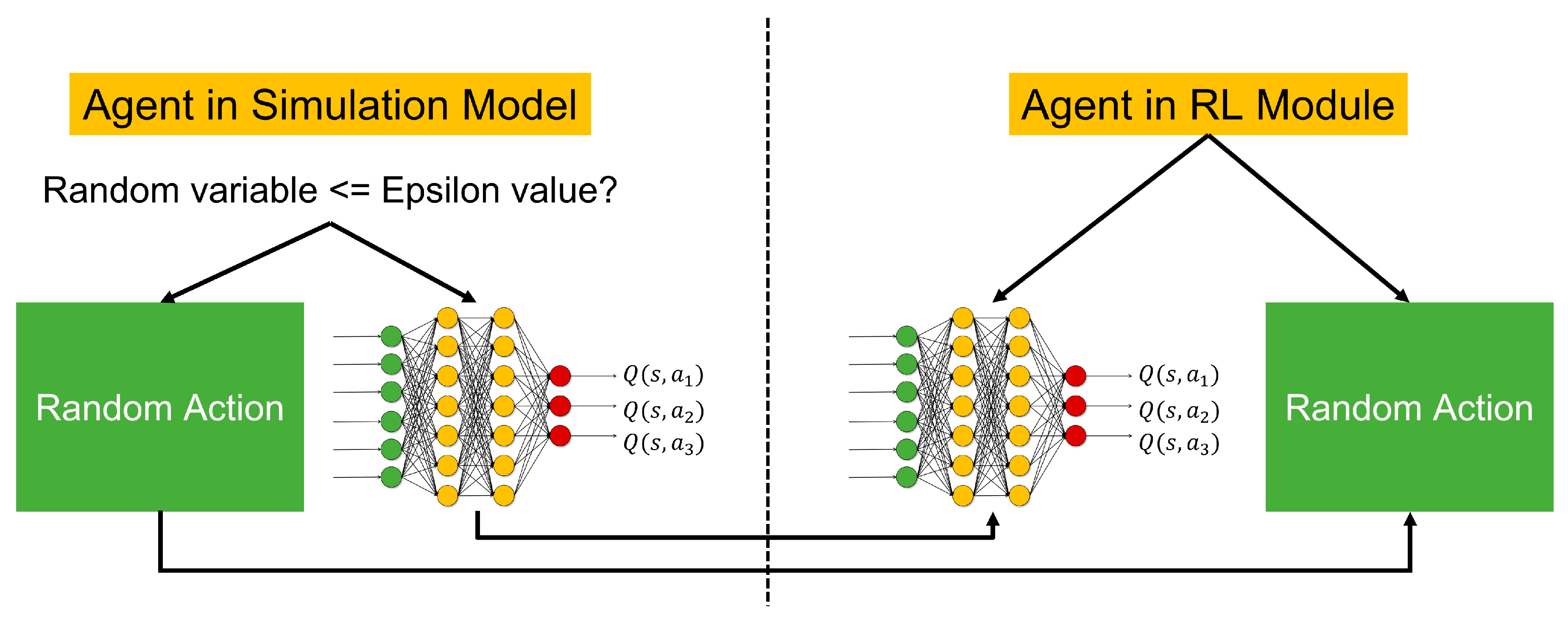
Step 4: The trained policy network is evaluated using the simulation model. The agent applies the epsilon-greedy (e-greedy) policy [33,34] when selecting an action to prevent local optimization of the objective function. Therefore, the agent in the simulation model randomly selects an action when it (i.e., a randomly generated number) is smaller than the epsilon value, whereas it selects the action with the largest value based on the policy network when it is larger than epsilon. The RL module has the same agent and policy network as the simulation model and updates its policy network by copying the network parameters from the simulation after a simulation run is completed. Accordingly, the RL agent can replicate the same action as the simulation model and receives the same reward as the simulation model. The conceptual diagram of the action–selection criterion of the agent in the simulation model and the replication of the policy network of the simulation into the RL module are shown in Figure 6.

Step 5: The simulation results are recorded in a table in the simulation model until the simulation is executed and completed. Each row of the table represents an index divided by a certain time interval in the time window. The simulation control module collects the state, action, and reward dataset of the re-entrant production line recorded throughout the simulation and transmits it to the RL module to perform training.

Step 6: This study uses the DDQN algorithm to address the problem of overestimating the values of actions, which frequently occurs with the original DQN algorithm. The DDQN algorithm maintains two networks (main and target networks) and uses them separately for different purposes. The target network is used to select an action during training; the main network is used to estimate the value of an action. 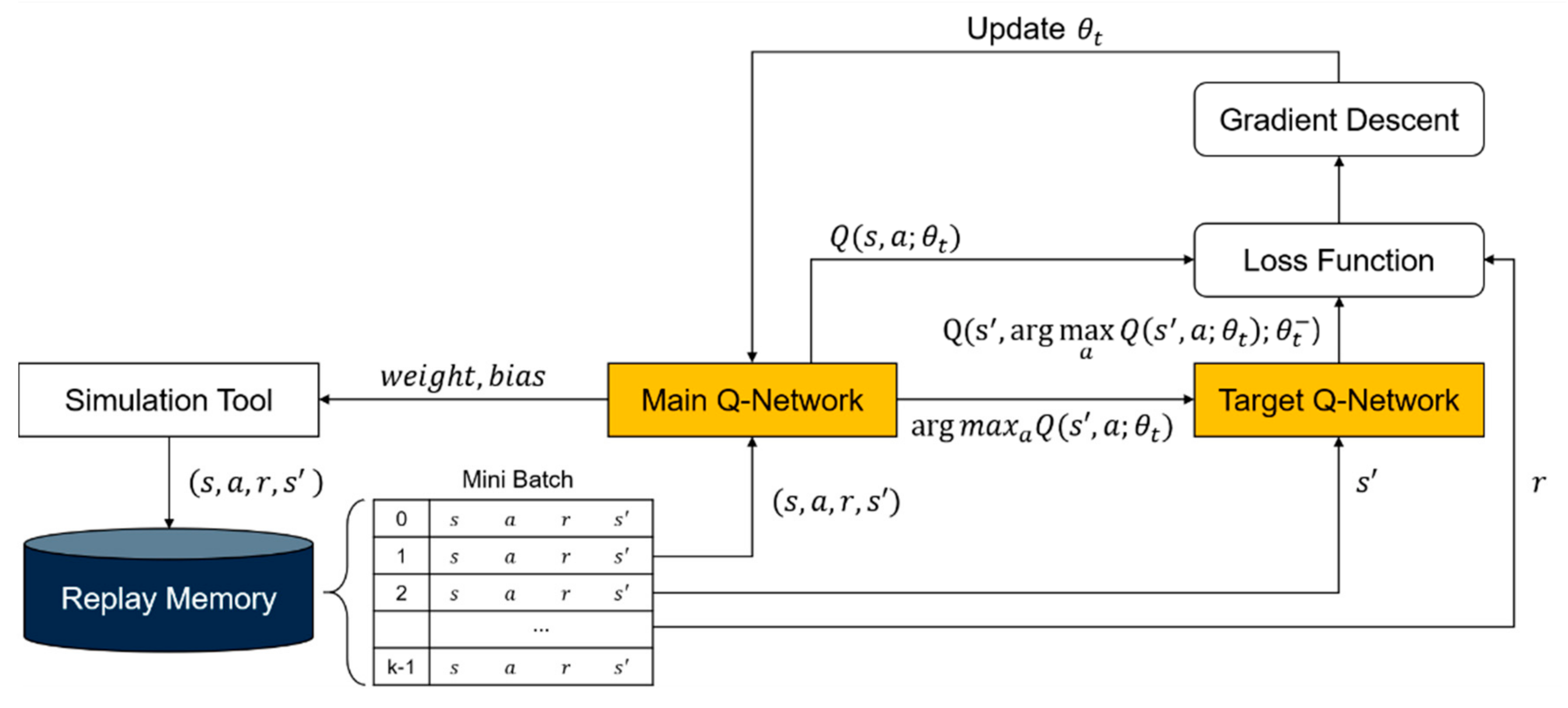This feature enables the DDQN algorithm to deliver better learning outcomes than the original DQN algorithm in various environments, including probabilistic factors [35,36]. The DDQN-based policy network update structure is shown in Figure 7. The input data are the state ($s$), action ($a$), reward ($r$), and transition of the next state ($s^{\prime }$) observed by the agent in the simulation model. Each transition is stored in the replay memory. The policy network is updated by mini-batch learning by randomly extracting the transitions stored in the replay memory. The time-sequence dependence can be resolved by mini-batch learning. Finally, the weight and bias parameters are transmitted from the updated policy network to the simulation tool. Algorithm 1 presents the pseudocode of the DDQN-based learning steps performed in the RL module. First, each variable used for the calculation is declared, and the policy network is initialized. The data obtained by the RL-based dispatching of vehicles are collected from the simulation model, and the data are organized into the state, action, reward, and transitions of the next state, which are stored in the replay buffer. DDQN-based learning is performed by sampling from the replay buffer. The ending rule in the pseudocode, as shown in Algorithm 1, is designed to be adaptive to the training performance. Specifically, the ending count increases only when the reward of the current episode is within the top 25% of historic rewards since the training procedure starts. The learning is repeatedly performed until the termination condition is achieved.

Algorithm 1 DDQN-based scheduling algorithm

1: Declarations: episode $EP$, index of ending rule $E$, sum of step reward of episode $R^{EP}$

2: Initialization: Set main network $Q_{\theta }$ with random weight $\theta$, target network $Q_{{\theta }^{\prime }}$ with ${\theta }^{\prime }$ = $\theta$, replay buffer $D$, reward buffer $D^R$

3: Body:

4:  GET the trajectory $EP$ from DES control module with RL-based production control

5:  while $e$ $<$ $E$ do:

6:   for $t=1,\dots ,T$ do:

7:    Store transition ($s_t$, $a_t$, $r_t$, $s_{t+1}$) in replay buffer $D$

8:   end for

9:   for $i=1,\dots ,I$ do:

10:   Sample transition ($s_i$, $a_i$, $r_i$, $s_{i+1}$) $~D$

11:    Compute target $Q$ value:

12:     $Q^{\ast }\left(s_i,a_i\right)\approx r_i+\gamma Q_{\theta }\left(s_{i+1},argma{x}_{a^{\prime }}{Q}_{{\theta }^{\prime }}\left(s_{i+1},a^{\prime }\right)\right)$

13:    Perform gradient descent step on ${\left(Q^{\ast }\left(s_i,a_i\right)-Q_{\theta }\left(s_i,a_i\right)\right)}^2$

14:    Update target network $Q_{{\theta }^{\prime }}$ parameters:

15:     ${\theta }^{\prime }\leftarrow \tau \ast \theta +\left(1-\tau \right)\ast {\theta }^{\prime }$

16:   end for

17:   if $R^{EP}<$ getQuarterValue($D^R$) then:

18:    $e=e+1$

19:   else:

20:    $e=0$

21:   end if

22:   Store $R^{EP}$ in reward buffer $D^R$

23:   if $e\ne E-1$ then:

24:    GET the trajectory $EP$ from DES control module with agent

25:   else:

26:    POST the weights and biases of the final agent

27:   end if

28:  end while

3.3. System Module-Integration Procedure

The integration procedure of the RL and DES control modules can be viewed as communication between a client and a server, as shown in Figure 8. The RL module acts as the client and requests data for training. The DES control module acts as the server, which executes the simulation model, collects the data, and transmits them to the RL module. First, the RL module requests the state, action, and reward values to initialize the policy network. The DES control module executes the simulation of the target system. Once the simulation is completed, the state, action, and reward values are collected and transmitted to the RL module. This process is repeated until a preset count is reached, and the best-performed episode is used to initialize the policy network with which the training procedure begins. The DRL module performs training, and the learned weights and biases are transmitted to the DES control module, which subsequently executes the simulation software by reflecting the trained weights and biases. Once the simulation is completed, the state, action, and reward values are transmitted back to the RL module by the DES control module, and training is performed. Once the weights and biases of the policy network converge by the repeated interaction between the RL and DES control modules, the DES control module reflects and stores the last policy network in the simulation model. In this study, the DES control module is written in C# and the RL module in Python with Pytorch. Their communication is achieved by a TCP/IP interface.

3.4. DES Control Module Class

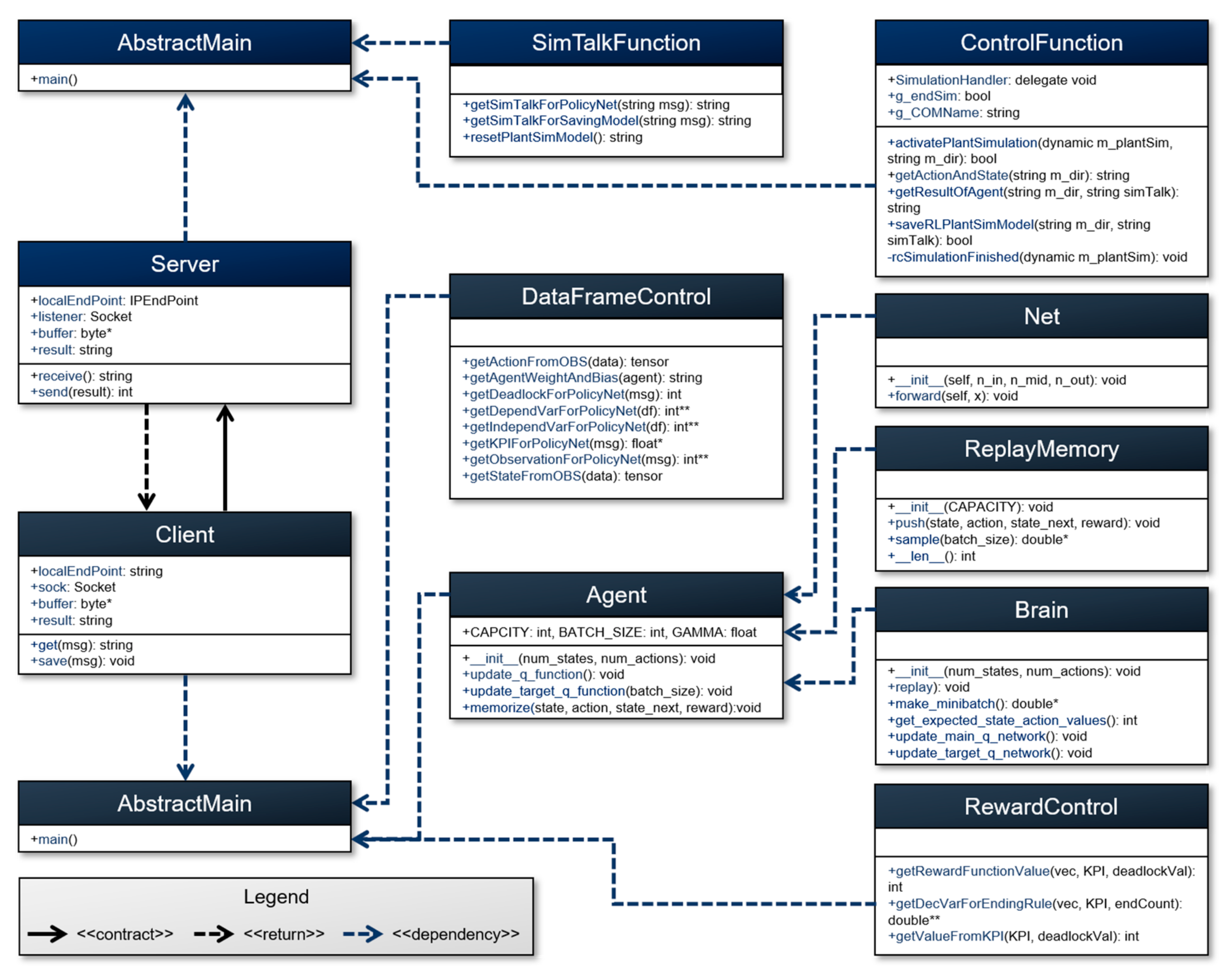
The class diagram to explain the classes created to implement each module in the scheduling system is presented in Figure 9. The DES control module is composed of AbstractMain, TCP/IP Server, SimTalkFunction, and ControlFunction classes. First, the server is activated by the TCP/IP server class for data exchange. Subsequently, the simulation engine is operated by the ControlFunction class and the production line model is loaded. Following this, the trained network parameters including the weight and bias data transmitted from the RL module by the SimTalkFunction class are reflected. The ControlFunction class implements the simulation and collects data once the shutdown event is triggered. Finally, the simulation engine is shut down and the data collected by the TCP/IP server class are returned to the RL module.

The RL module is composed of AbstractMain, TCP/IP Client, DataFrame Control, Agent, Net, ReplayMemory, and Brain classes. First, data are transmitted from the TCP/IP Server class of the DES control module by the TCP/IP Client class. The transmitted data are preprocessed for training by the DataFrameControl class. The Agent class receives the number of state variables and action types and creates an instance of the Brain class for the DDQN algorithm-based learning. It creates the main and target Q-networks by the Net class and stores the data preprocessed by the ReplayMemory class in the memory. The DDQN algorithm is executed by the Brain class, the learned weight and bias data are transmitted to the DES control module by the TCP/IP Client class, and the data required for training by simulation are requested to be returned.

4. Experimental Design and Results

This section reports the experiments conducted to verify the applicability and effectiveness of the proposed DRL-integrated scheduling system. The experiments are divided into three cases. Case A is for the makespan comparison with the results of single priority-based dispatching rules. Case B investigates the impact of part sequences. Case C is for the analysis of flexibility effects. All experiments are performed in Windows 10 running on a laptop with an Intel Core i7 vPro processing unit at 4.8 GHz and 16 GB memory.

4.1. Case A

The makespans of the proposed DRL-integrated scheduling system and single dispatching rules are compared in Case A. The proposed scheduling system operates by combining three single dispatching rules and choosing one rule as an action for each state of the re-entrant production line such that the accumulation of future rewards is maximized. The simulation settings for Case A are listed in

Table 2. Availability and mean time to repair settings of each station in Case A.

Process No.	Process	Availability (%)	Mean Time to Repair (Min)
1	Body side weather strip	90	10
2	Main body wire harness	90	10
3	Sunroof	90	10
4	Roof rail air bag	90	10

and

Table 3. Processing time settings of each product in Case A.

Product	Production Plan	Body Side Weather Strip (Min)	Main Body Wire Harness (Min)	Sunroof (Min)	Roof Rail Air Bag (Min)
Car A	100	1.0	0.9	1.8	1.0
Car B	100	0.9	0.8	0.0	0.9
Car C	100	1.2	1.0	0.0	1.2
Car D	100	1.1	1.1	2.0	1.1

.

Totally, 50 experiments are conducted and the distribution of the makespan is shown in a boxplot graph in Figure 10. As summarized in

Table 4. Makespan mean value comparison in Case A.

Single Dispatching Rule (Time)			DRL (Time)
FCFS	FOPR	MOPR	DDQN
12:29:31 (+15%)	14:58:33 (+29%)	11:41:06 (+9%)	10:37:25

, the average makespan using the proposed system is 15%, 29%, and 9% smaller than those from the FCFS, FOPR, and MOPR rules, respectively. Note that the proposed system has the smallest variance, i.e., the proposed system yields more robust and consistent results than any single dispatching rule.

4.2. Case B

In Case B, three sequences—random, batch, and fixed sequences—are compared in terms of the makespan to investigate the impact of the sequence on the proposed system. The Case B experiment is important because it helps identify the best sequencing method for the proposed scheduling system. The random sequence is defined as a random arrangement of vehicles coming from the preceding process line. In the batch sequence, vehicles are arranged in the form of a batch if they are of the same model (i.e., have the same build sequence and processing time). The fixed sequence is defined as a repetition of a specific sequencing pattern (e.g., 1→2→3→4→1→2→3→4→1→2→3→4→…). The Case B experimental settings are the same as those in Case A, which are listed in Table 2 and Table 3.

The RL training procedure converges all sequences to their optimal policies and the results are reported in

Table 5. Reward value and makespan comparison in Case B.

	Random Sequence	Batch Sequence	Fixed Sequence
Reward Value (num)	−57	−54	−67
Makespan (time)	10:04:21	11:10:45 (+11%)	10:09:41 (+1%)

. The fixed and random sequences receive relatively large rewards, whereas the batch sequence receives a small reward. Similarly, from the makespan perspective, the batch sequence shows the worst performance. It can be inferred that the random sequence performs well with the proposed scheduling system because it shows higher flexibility in terms of the vehicle sequence than the other sequencing rules. The learning convergence is shown in Figure 11.

4.3. Case C

It is important to investigate the impact of flexibility on the proposed scheduling system because the underlying production line, i.e., the re-entrant production line, originally intends to comply with the high-flexibility requirement. Therefore, the learning time and makespan changes by varying the flexibility of the re-entrant production line are examined using the proposed scheduling system in Case C. The difference in the flexibility of the re-entrant production line is manipulated by adding a multipurpose station. For this experiment, metrics to measure the degree of flexibility are needed to appropriately measure the performance of the comparative models. For measuring the degree of flexibility, two metrics are introduced based on previous studies on the quantification of flexibility [37,38,39,40]: operation flexibility (OF) and routing flexibility (RF).

OF represents the ability to interchange the order of operations. Given that a group of products follows the same order of processes, OF of the product group can be measured as the ratio of alternative precedence graphs to the maximum possible number of alternative precedence graphs. This is expressed as follows.

$$OF\left(\%\right)=100\times \frac{countofalterativeprededencegraphs}{\left(countofoperations\right)!}$$

(3)

For example, if a product needs four processes, the maximum possible number of alternative precedence graphs is 4!. Assuming that all four processes are independent, the order of operations can be ignored. Therefore, the number of alternative precedence graphs is 24. In this case, OF is equal to 100% (= $100\times \frac{\left(24\right)}{4!}$).

RF is defined as an ability to account for machine unavailability. RF can be achieved utilizing multipurpose machines, which realize alternative routes for parts that encounter unavailable machines. Conceptually, RF equals the average number of machines that can perform an operation, as expressed in Equation (4).

$$RF\left(\%\right)=100\times \frac{{{\displaystyle \sum }}_{u=1}^n\left|I\left(u\right)\right|}{m\times n}$$

(4)

where $u$ is the index of operations and $m$ and $n$ represent the total number of machines and the total number of operations, respectively. $I\left(u\right)$ represents the index set of the machines that can perform operation. For example, assume that a system has four machines (i.e., $m=4$) and a product needs four processes (i.e., $n=4$). Under this assumption, if one machine exercises only one process uniquely, RF is 25% (= $100\times \frac{\left(1+1+1+1\right)}{16}$). However, if each machine operates all four processes commonly, RF is 100% (= $100\times \frac{\left(4+4+4+4\right)}{16}$).

Two hypothetical re-entrant production lines are modeled by varying the degree of flexibility, as shown in Figure 12. The OF for both production lines is the same, i.e., 100%, as the vehicles have interchangeable job sequences. The left model in the figure has 25% RF because each station is dedicated to only one process. However, the right model has 50% RF owing to the addition of a multipurpose station that can perform all four processes. The experimental settings applied in Case C are listed in

Table 6. Availability and mean time to repair settings of each station in Case C.

Process Number	Process	Availability (Unit: %)	Mean Time to Repair (Unit: Min)
1	Body side weather strip	90	10
2	Main body wire harness	90	10
3	Sunroof	90	10
4	Roof rail air bag	90	10
5	Universal Machine	100	0

. Note that the processing time settings of all products are the same as in Cases A and B.

Figure 13 shows the learning curve and simulation throughput results for Case C. When the multipurpose station is added to the model, although a larger reward value is received, approximately 100 additional episodes are required for the reward values to converge. However, notably, the average makespan is reduced by 28%, based on the makespan box plot in Figure 13 and

Table 7. Learning time and makespan mean value comparison in Case C.

	Line (OF = 100%, RF = 25%) with DRL	Line (OF = 100%, RF = 50%) with DRL
Learning time (unit: time)	3:13:42 (+14%)	2:46:12
Makespan mean value (unit: time)	10:37:25 (+28%)	7:39:16

. Thus, although the overall complexity is increased by adding the multipurpose station, the makespan is significantly reduced because of the increased flexibility. Specifically, the increase in flexibility mitigates the negative impact of the increase in complexity. In addition, as the multipurpose station reduces the makespan, the total training time becomes shorter.

5. Conclusions

An increasing number of manufacturing companies are making efforts to utilize highly flexible production systems, including re-entrant production lines, in which jobs visit specific facilities or stations more than once to increase system utilization with limited resources. However, the execution of re-entrant production lines is more complex than those of general manufacturing systems because predicting the arrival of jobs is difficult owing to the high degree of uncertainty in a dynamic manufacturing environment. In this study, DRL with the capability of a short computation time and global optimization was used to solve the complex re-entry production line scheduling problem.

A DRL-integrated scheduling system was implemented in which the makespan was used as the operation performance index and the state, action, and reward were defined according to the characteristics of the problem. A hypothetical re-entrant production line was modeled using a DES tool, which is advantageous in providing a model-free learning environment by reasonably modeling the uncertainty in a dynamic manufacturing system. A DRL model for scheduling was trained using the DDQN algorithm, and the configuration and system architecture of the entire training system were established. Unlike studies conducted in the existing literature, the system proposed in this paper could obtain more accurate and realistic scheduling results in complex and dynamic manufacturing systems by using simulation models as learning environments. The makespan obtained from the simulation results was used as a performance index for DRL by representing the manufacturing system or production line in detail through the simulation model.

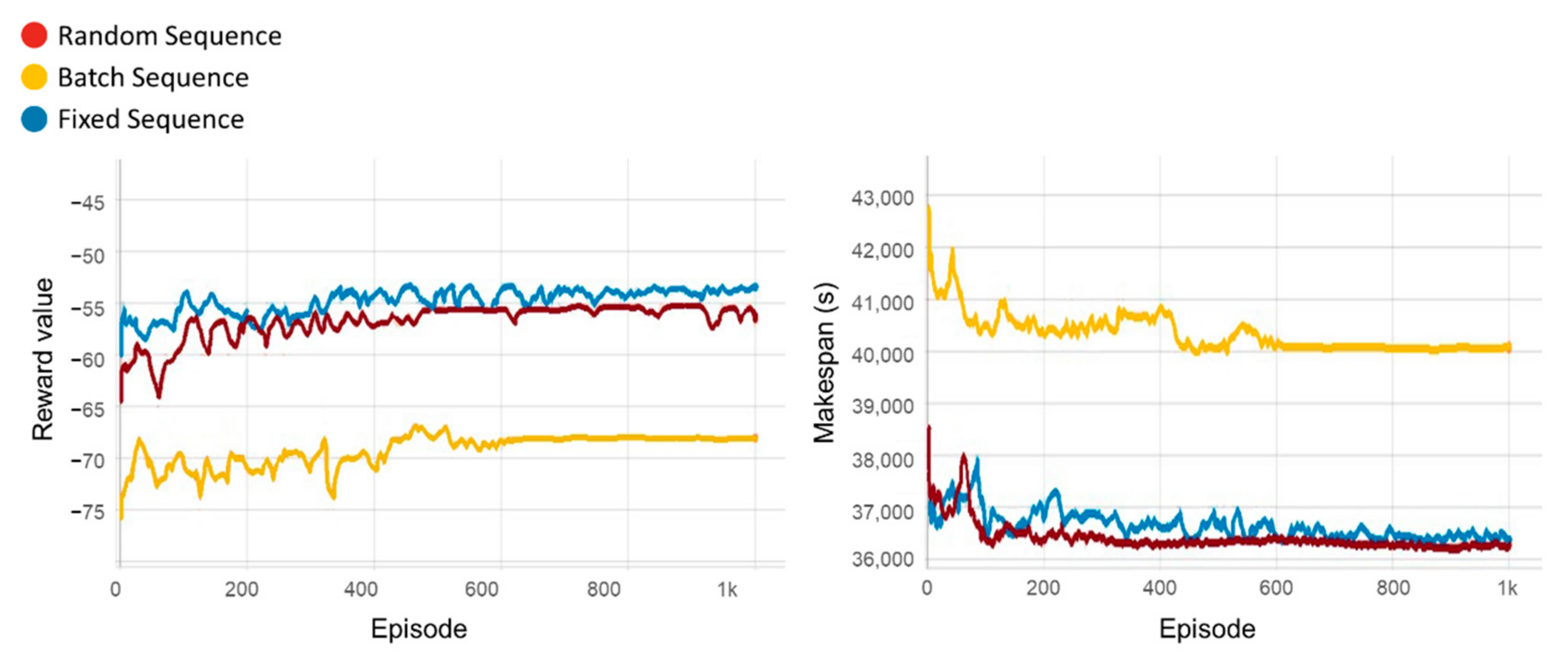
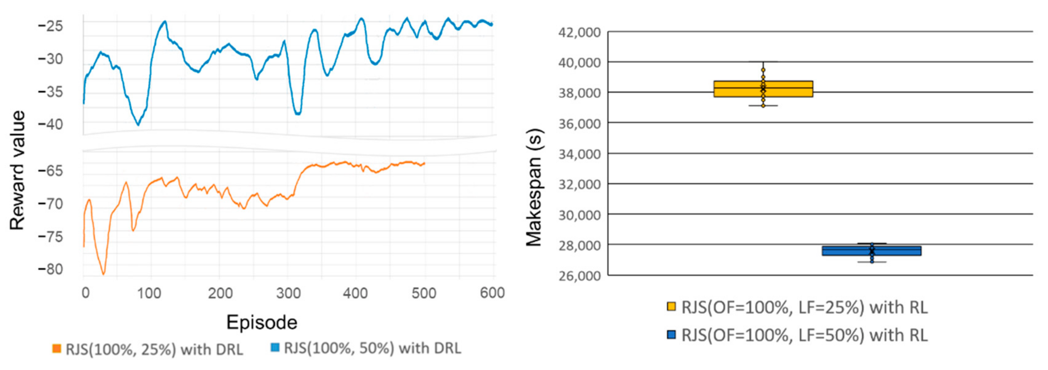
Various experiments were conducted to verify the operational performance of the re-entrant production line compared to those of priority-based single dispatching rules. In addition, the proposed scheduling system was assessed with different job sequences and different flexibility cases.

There are several directions for future studies. First, this study manually modeled a re-entrant production line for the RL agent using a simulation tool, i.e., the model cannot be updated dynamically whenever the actual production line is changed. Therefore, as a future research topic, digital twin technologies to automatically generate and synchronize a training model with actual production lines can be explored. Second, this study trained the RL agent based on rewards for its actions using a fixed time interval to collect the rewards periodically. Because the effectiveness of a fixed time-based immediate reward in representing the global cost function is unknown, a future study could focus on designing another reward structure that can better represent the global cost function. Finally, this study focused on determining the order of product input considering only makespan, but it can be expected to develop into a more complex and applicable system for dynamic manufacturing sites through various evaluation indicators throughout operation such as line utilization, failure rate, waiting rate, bottleneck, etc. The performance of the proposed system will be more sophisticated and decision-makers will be able to check the scheduling results from more diverse perspectives.

Abbreviations

List of symbols used in this paper.

$\rho$	Criterion for measurement of the production time interval.
$k$	Index of the products that completed the production process ($k=1,\dots ,K$).
$i$	Index of the interval divided by criterion $\rho$ in the time window ($i=1,\dots ,I$).
${\mu }_{i_k}$	Production completion time of the $k$th product in the $i$th period.
$N_i^{\rho }$	Number of products completely produced in the $i$th period measured by criteria $\rho$ in the time window.
$N_j$	Number of jobs.
$r_i$	Step (or immediate) reward of the $i$th period.