Abstract
Moment-based methods can measure the safety degrees of mechanical systems affected by unavoidable uncertainties, utilizing only the statistical moments of random variables for reliability analysis. For the conventional derivation of the first four statistical moments based on the second-order Taylor expansion series evaluated at the most likelihood point (MLP), skewness and kurtosis involve the higher fourth raw moments of random variables and thus are unfavorable for engineering applications. This paper develops new computing formulae for the first four statistical moments which require only the first four central moments of random variables, and the probability distribution of the performance function is approximated using cubic normal transformation. Several numerical examples are given to demonstrate the accuracy of the proposed methods. Comparisons of the two proposed approaches and the maximum entropy method (ME) are also made regarding reliability assessment.
1. Introduction
The performance of mechanical systems is often affected by unavoidable uncertainties. Moment-based methods, as some of the most important reliability methods, can measure the safety degrees of mechanical systems by considering these uncertainties. The commonly used moment-based methods [1,2,3,4,5] can be divided into two categories: (1) second-order moment methods [2,3] and (2) high-order moment methods [4,5]. Second-order moment methods utilize only the first two statistical moments of a performance function, and thus their computing formulae are very simple. Nevertheless, second-order moment methods are not precise, because the first two statistical moments insufficiently recover the probability distribution of the performance function.
High-order moment methods have therefore been put forward to improve precision. These methods involve the estimation of high-order statistical moments and the approximation of probability distributions [6]. For the estimation of high-order statistical moments, two kinds of methods so far have been developed to calculate high-order statistical moments [7]. The first kind is the dimension-reduction method (DRM), which is capable of decomposing a multivariate function into the sum of several functions for a low-dimensional vector [8]. Although the univariate dimension-reduction method (UDRM) [9] can provide more accurate moment estimation than the first- and second-order Taylor expansion series, the UDRM may result in error due to a small residual error in the first moment for a system involving high nonlinearity or arbitrarily large numbers of random variables. To eliminate this drawback, Zhang and Pandey [10] developed a novel multiplicative UDRM (M-UDRM) based on the ME principle and fractional moments which is theoretically more accurate than the UDRM. Even so, the M-UDRM may still fail when faced with nonlinear problems. Xu and Rahman [11] proposed the bivariate dimension-reduction method to reduce the residual as much as possible. Nevertheless, its disadvantage is that it sacrifices some computational efficiency to improve precision. Xu and Zhou [12] put forward an adaptive trivariate DRM which strikes a balance between precision and efficiency. The second kind is the point-estimate method, which is able to decompose the statistical moment into a weighted summation of the performance function at several designated locations [13]. Although two-point-estimate methods are very efficient, the estimating points may be beyond the region of the probability distribution. Thus, Zhao and Ono [14] put forward a novel point-estimate method for statistical moment estimation, where the number of estimating points separated from the original variable is easily improved, yet there are enough estimating points to ensure precision for random variables with large variances. Zhou and Lu [15] put forward a sparse grid-based approach to select the sampling points for estimating statistical moments, the features of which (automatic sampling, special interpolation process and dimension adaptability) make numerical integration very flexible and very efficient. Approximating the probability distribution of the performance function is another key objective when the first four moments are obtained. The existing approaches to approximating probability distributions mainly include the Johnson system, the Pearson system, the Burr system and ME [16,17]. Nevertheless, these existing approaches always have incompatibility restrictions. The Johnson, Pearson and Burr systems are invalid at the interfaces between different distribution types. ME employs truncated exponential polynomials that cannot contain all distribution types.
From the above literature review, it can be seen that the accuracy of high-order statistical moments mainly depends on the expanded form of the performance function and the computational difficulty of high-dimensional numerical integration. The accuracy in approximating a probability distribution mainly depends on adaptability to different distribution types. Compared with the Taylor expansion series evaluated at the most probable point (MPP) [18,19], the Taylor expansion series evaluated at the MLP avoids the iteration of nonnormal-to-normal transformation to further improve the accuracy of the high-order statistical moments. The computational formulae for the first four statistical moments based on the Taylor expansion series evaluated at the MLP are merely applicable to the first-order form. For the second-order Taylor expansion series evaluated at the MLP, the first four statistical moments of the performance function have not yet been reported. According to the conventional derivation, the computational formulae for the skewness and kurtosis of the performance function involve the higher fourth raw moments of random variables and thus are unfavorable for engineering applications.
The innovation of the paper is the development of new computing formulae for the first four statistical moments based on the second-order Taylor expansion series evaluated at the MLP, which merely requires the first four central moments of random variables. Furthermore, the paper proposes an efficient high-order-moment-based reliability method by combining the MLP and cubic normal transformation [20]. The remainder of the paper is organized as follows: Section 2 reviews cubic normal transformation; Section 3 and Section 4 present the details about the two proposed methods; Section 5 provides several numerical examples; and conclusions are drawn in the final section.
2. Overview of Cubic Normal Transformation
It is generally known that X with an arbitrary distribution is standardized by using its mean and standard deviation, and the standardized form of X is expressed as:
where is the standardized random variable; and are the mean and standard deviation of X, respectively.
According to cubic normal transformation [21], the standardized random variable is formulated as:
where Z is the standard normal random variable; a, b, c and d are polynomial coefficients.
Substituting Equation (1) into (2), X is written as:
3. The Proposed Approach 1
The performance function is linearized at the MLP of the original random space directly. Based on the integral formulae for statistical moments, the first four central moments of the performance function are calculated. Cubic normal transformation is utilized to approximate the probability distribution of the performance function. In order to facilitate the description, the proposed method 1 is called FOPM + MPL, and its flowchart is shown in Figure 1. FOPM + MPL does not require any “nonnormal to normal” transformation to search the MPP and achieve high accuracy.
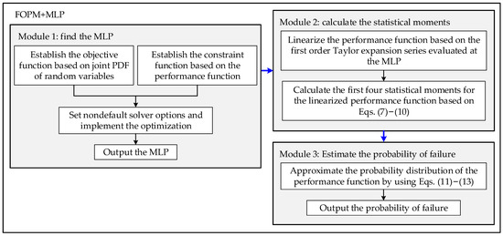
Figure 1.
Flowchart of the proposed approach 1.
The MLP of the original random space is restricted by two conditions: (1) the MLP maximizes the joint probability density function (PDF) of X; and (2) the MLP is subjected to the limit state equation g(X) = 0. Thus, the MLP is determined by the following model as:
where is the joint PDF of X evaluated at . The performance function g(X) is linearized based on the first-order Taylor expansion series evaluated at as follows:
where is the gradient vector of g(X) evaluated at . Equation (5) can also be rewritten as follows:
where and . According to the property of a linear combination of , the first four statistical moments of g(X) are formulated as:
where , , and are the mean, standard deviation, skewness and kurtosis of g(X), respectively; , , and are the first four central statistical moments of , respectively. According to Equation (3), the performance function g(X) can be reduced to a cubic function of Z as:
Based on the principle of isoprobabilistic transformation, the cumulative distribution function (CDF) of g(X) is given as:
where is the CDF of the standard normal random variable; is the solution nearest to the origin for the following equation as:
4. The Proposed Approach 2
Although the performance function is approximated based on the second-order Taylor expansion series evaluated at the MLP to further improve the precision, the formulae for the first four statistical moments for the performance function in quadratic form are very complicated. In order to facilitate the description, the proposed method 2 is called SOPM + MPL, and its flowchart is shown in Figure 2. Different from the second-order Taylor expansion series evaluated at the MPP, the skewness and kurtosis of the performance function for SOPM + MPL involve the higher fourth raw moments of random variables. The highlight of SOPM + MPL is that the higher fourth raw moments of random variables are approximated using a series of the first four central moments.
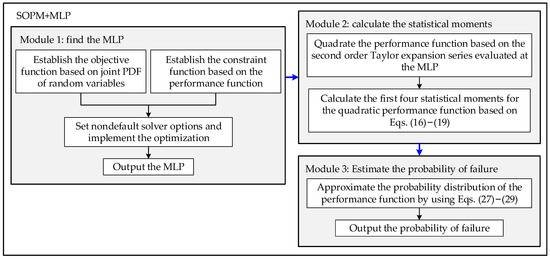
Figure 2.
Flowchart of the proposed approach 2.
Without loss of generality, the performance function g(X) is approximated based on the second-order Taylor expansion series evaluated at the MLP as follows:
where is the Jacobi matrix of evaluated at . Equation (14) can also be rewritten as follows:
where ; ; ; .
According to the definition of central moments, the first four statistical moments of g(X) are formulated as:
where are the kth raw moments and are respectively formulated as:
Since the higher-order moments of random variables are difficult to obtain, are all set to zero. Equations (23) and (24) are also approximated as:
Substituting Equations (20)–(22) and Equations (25) and (26) into Equations (16)–(19), the first four statistical moments of g(X) can be expressed as a function of , , and .
According to Equation (3), the performance function g(X) can be reduced to a cubic function of Z as:
Based on the principle of isoprobabilistic transformation, the cumulative distribution function (CDF) of g(X) is given as:
where is the CDF of the standard normal random variable; is the solution nearest to the origin for the following equation, as:
5. Illustrative Examples
In this section, three numerical examples are illustrated to demonstrate the efficiency and accuracy of the proposed method. The first numerical example considers the linear performance function with input variables following the standard exponential distribution. The nonlinear performance function of a reinforced concrete beam considering bending moment safety is discussed as the second example. Example 3 shows the reliability analysis of the implicit performance function.
5.1. Example 1: Linear Performance Function
The following performance function is given as:
where n = 2; a is a constant; and all obey the standard exponential distribution.
From Table 1 and Table 2, it can be seen that the first four statistical moments of the linear performance function with the different constants calculated by FOPM + MLP, SOPM + MLP and ME are the same in this example. Moreover, Figure 3 illustrates the tails of the recovered PDF of the linear performance function with the different constants approximated by cubic normal transformation and ME based on the first four statistical moments. It can be seen that the recovered PDF tails of the linear performance function approximated by cubic normal transformation are almost the same as those of the linear performance function approximated by Monte Carlo simulation (MCS), while the recovered PDF tails of the linear performance function approximated by ME are quite different from those of the linear performance function approximated by MCS.

Table 1.
MLP and the first four statistical moments calculated by the different methods for Example 1.

Table 2.
Relative errors of the first four statistical moments calculated by FOPM + MLP, SOPM + MLP and ME.
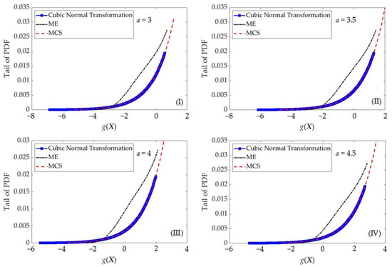
Figure 3.
Tails of PDFs approximated by the different methods in Example 1.
Figure 4 shows the failure probabilities of the linear performance function with the different constants calculated by the different methods. Compared with MCS, FOPM + MLP and SOPM + MLP have high accuracy. However, the failure probabilities estimated by ME do not match well those estimated by MCS. The reason for the higher precision of FOPM + MLP and SOPM + MLP compared with ME is that their accuracy in approximating the probability distribution based on cubic normal transformation is higher than that of ME, given the same first four moments of the performance function in this example.
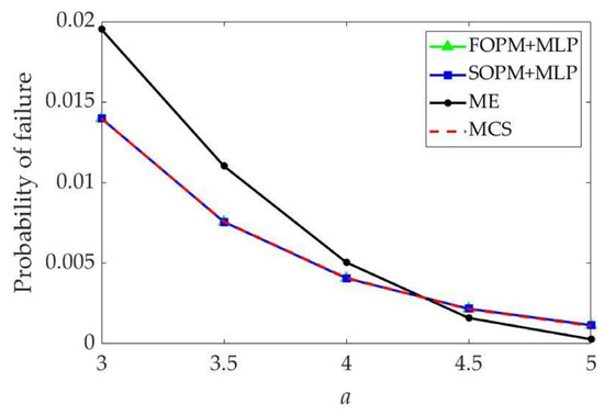
Figure 4.
Comparison of the failure probabilities estimated by the different methods for Example 1.
5.2. Example 2: Nonlinear Performance Function
The nonlinear performance function of a reinforced concrete beam considering bending moment safety is expressed as follows:
where D is the effective depth of the reinforcement; Ts is the yield stress of the reinforcement; As (= 2.5 × 10⁻⁴ m2) is the area of reinforcement; K (=0.5) is a coefficient related to the stress–strain relationship of concrete; Sb (=0.15 m) is the cross-sectional width; Tc is the concrete’s maximum compressive strength; Mb is the sectional bending moment. The statistical information for these random variables is provided in Table 3.

Table 3.
Statistical information for the random variables in Example 2.
From Table 4, it can be seen that the first four statistical moments of the nonlinear performance function calculated by FOPM + MLP are quite different from those of the nonlinear performance function calculated by MCS in this example. It can be seen from Table 5 that the mean and kurtosis of the nonlinear performance function calculated by SOPM + MLP are much closer to those of the nonlinear performance function calculated by MCS, while the standard deviation and skewness of the nonlinear performance function calculated by ME are much closer to those of the nonlinear performance function calculated by MCS.

Table 4.
MLP and the first four statistical moments calculated by the different methods for Example 2.

Table 5.
Relative errors of the first four statistical moments calculated by SOPM + MLP and ME for Example 2.
Figure 5 shows that the failure probabilities for the nonlinear performance function calculated by the different methods vary with the threshold. The probabilities of failure estimated by MCS with 106 samples are regarded as reference solutions. It is clear that the results estimated by FOPM + MLP and SOPM + MLP are closer to the reference solutions than those estimated by ME. Furthermore, SOPM + MLP has a higher accuracy than FOPM + MLP. The accuracy of SOPM + MLP is higher than that of FOPM + MLP for the nonlinear performance function, the accuracy of the second-order Taylor expansion series evaluated at the MLP being higher than that of the first-order Taylor expansion series evaluated at the MLP.
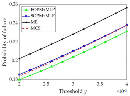
Figure 5.
Comparison of the failure probabilities estimated by the different methods in Example 2.
5.3. Example 3: Implicit Performance Function
Figure 6 represents the main shaft device of a multi-layer winding hoist subjected to various rope tensions which has seven dimensional variables and three loading variables. The statistical information for these random variables is provided in Table 6. The implicit performance function is given as:
where Q = 716 MPa is the structural strength of the main shaft device; S(X) is the maximum stress of the main shaft device, which is obtained by combining the finite element method and the Kriging surrogate model.
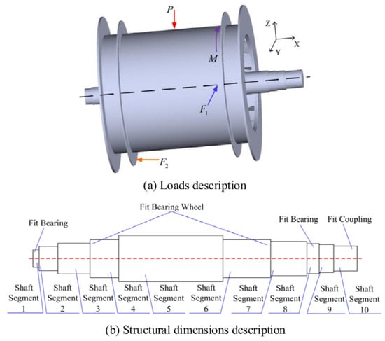
Figure 6.
Main shaft device of a multi-layer winding mine hoist for Example 3.

Table 6.
Statistical information for the random variables in Example 3.
Table 7 shows the probability of failure estimated by FOPM + MLP, SOPM + MLP, ME and MCS. The results indicate that the failure probability estimated by SOPM + MLP is the closest to that estimated by MCS, and the relative error between the failure probability estimated by SOPM + MLP and that estimated by MCS is merely −0.07%.

Table 7.
Comparison of the failure probabilities for Example 3.
6. Conclusions
This paper has presented efficient high-order-moment-based reliability methods by combining the MLP and cubic normal transformation, these being named FOPM + MLP and SOPM + MLP. The main conclusions drawn are as follows:
- (1)
- Compared with the traditional moment-based methods, the proposed methods employ the Taylor expansion series evaluated at the MLP to avoid the iteration of nonnormal-to-normal transformation and further improve the accuracy of high-order statistical moments. Moreover, based on the second-order Taylor expansion series evaluated at the MLP, the proposed new computing formulae for the first four statistical moments require only the first four central moments of random variables and are beneficial with respect to engineering applications.
- (2)
- Through two engineering examples—that of the reinforced concrete beam and that of the main shaft device of the mine hoist—the proposed SOPM + MLP is capable of effectively evaluating reliability in comparison with MCS. Furthermore, the proposed SOPM + MLP lays the foundation for the next reliability-based robust optimization design.
- (3)
- Although the accuracies of the proposed methods were improved given the known statistical moments of the random variables, the proposed methods still have some limitations. When encountering performance functions with complex forms, the proposed methods require multiple redesigns of the starting points to find the MLP and this greatly consumes computing time. When a few random samples of random variables can be obtained, the statistical moments of random variables are affected by the sample size and possess various uncertainties. Thus, the reliability calculated by the proposed methods will be inaccurate for engineering problems with only a few random samples.
Author Contributions
Conceptualization, S.C. and H.L.; methodology, S.C.; software, S.C.; validation, H.L.; formal analysis, H.L.; investigation, S.C.; resources, H.L.; data curation, H.L.; writing—original draft preparation, S.C.; writing—review and editing, H.L.; visualization, S.C.; supervision, H.L.; project administration, S.C.; funding acquisition, S.C. All authors have read and agreed to the published version of the manuscript.
Funding
This work was supported by the Future Scientists Program of China University of Mining and Technology (grant no. 2020WLKXJ024) and the Postgraduate Research & Practice Innovation Program of Jiangsu Province (grant no. KYCX20_1985)—a project funded by the Priority Academic Program Development of Jiangsu Higher Education Institutions (PAPD).
Data Availability Statement
Not applicable.
Conflicts of Interest
The authors declare no conflict of interest.
References
- Wang, C.; Zhang, H.; Li, Q.W. Moment-based evaluation of structural reliability. Reliab. Eng. Syst. Saf. 2019, 181, 38–45. [Google Scholar] [CrossRef]
- Huang, X.Z.; Li, Y.X.; Zhang, Y.M.; Zhang, X.F. A new direct second-order reliability analysis method. Appl. Math. Model. 2018, 55, 68–80. [Google Scholar] [CrossRef]
- Hu, Z.L.; Mansour, R.; Olsson, M.; Du, X.P. Second-order reliability methods: A review and comparative study. Struct. Multidiscip. Optim. 2021, 64, 3233–3263. [Google Scholar] [CrossRef]
- Lu, H.; Cao, S.; Zhu, Z.C.; Zhang, Y.M. An improved high order moment-based saddle point approximation method for reliability analysis. Appl. Math. Model. 2020, 82, 836–847. [Google Scholar] [CrossRef]
- Li, G.; He, W.X.; Zeng, Y. An improved maximum entropy method via fractional moments with Laplace transform for reliability analysis. Struct. Multidiscip. Optim. 2019, 59, 1301–1320. [Google Scholar] [CrossRef]
- Zhang, L.W. An improved fourth-order moment reliability method for strongly skewed distributions. Struct. Multidiscip. Optim. 2020, 62, 1213–1225. [Google Scholar] [CrossRef]
- Cao, S.; Chen, G.A.; Peng, Y.X.; Lu, H.; Ren, F.B. Uncertainty analysis and time-dependent reliability estimation for the main shaft device of a mine hoist. Mech. Based Des. Struct. Mech. 2022, 50, 2221–2236. [Google Scholar] [CrossRef]
- Zhang, Y.; Xu, J. Efficient reliability analysis with a CDA-based dimension-reduction model and polynomial chaos expansion. Comput. Meth. Appl. Mech. Eng. 2021, 373, 113467. [Google Scholar] [CrossRef]
- Rahman, S.; Xu, H. A univariate dimension-reduction method for multi-dimensional integration in stochastic mechanics. Probab. Eng. Eng. Mech. 2004, 19, 393–408. [Google Scholar] [CrossRef]
- Zhang, X.; Pandey, M.D. Structural reliability analysis based on the concepts of entropy, fractional moment and dimensional reduction method. Struct. Saf. 2013, 43, 28–40. [Google Scholar] [CrossRef]
- Xu, H.; Rahman, S. A generalized dimension-reduction method for multidimensional integration in stochastic mechanics. Int. J. Numer. Methods Eng. 2004, 61, 1992–2019. [Google Scholar] [CrossRef]
- Xu, J.; Zhou, L.J. An adaptive trivariate dimension-reduction method for statistical moments assessment and reliability analysis. Appl. Math. Model. 2020, 82, 748–765. [Google Scholar] [CrossRef]
- Hong, H.P. An efficient point estimate method for probabilistic analysis. Reliab. Eng. Syst. Saf. 1998, 59, 261–267. [Google Scholar] [CrossRef]
- Zhao, Y.G.; Ono, T. New point estimates for probability moments. J. Eng. Mech. 2000, 126, 433–436. [Google Scholar] [CrossRef]
- Zhou, C.C.; Lu, Z.Z.; Li, W. Sparse grid integration based solutions for moment-independent importance measures. Prob. Eng. Eng. Mech. 2015, 39, 46–55. [Google Scholar] [CrossRef]
- Zhang, Y.M. Principle of maximum entropy for reliability analysis in the design of machine components. Front. Mech. Eng. 2019, 14, 21–32. [Google Scholar] [CrossRef]
- Dai, H.Z.; Zhang, H.; Wang, W. A new maximum entropy-based importance sampling for reliability analysis. Struct. Saf. 2016, 63, 71–80. [Google Scholar] [CrossRef]
- Meng, Z.; Pu, Y.X.; Zhou, H.L. Adaptive stability transformation method of chaos control for first order reliability method. Eng. Comput. 2018, 34, 671–683. [Google Scholar] [CrossRef]
- Kang, B.; Mun, J.; Lim, J.; Choi, K.K.; Kim, D.H. Most probable failure point update method for accurate first-order reliability-based electromagnetic designs. J. Magn. 2019, 24, 408–412. [Google Scholar] [CrossRef]
- Peng, X.; Gao, Q.L.; Li, J.Q.; Liu, Z.Y.; Yi, B.; Jiang, S.F. Probabilistic representation approach for multiple types of epistemic uncertainties based on cubic normal transformation. Appl. Sci. 2020, 10, 4698. [Google Scholar] [CrossRef]
- Cao, S.; Lu, H.; Peng, Y.X.; Ren, F.B. A novel fourth-order L-moment reliability method for L-correlated variables. Appl. Math. Model. 2021, 95, 806–823. [Google Scholar] [CrossRef]
Publisher’s Note: MDPI stays neutral with regard to jurisdictional claims in published maps and institutional affiliations. |
© 2022 by the authors. Licensee MDPI, Basel, Switzerland. This article is an open access article distributed under the terms and conditions of the Creative Commons Attribution (CC BY) license (https://creativecommons.org/licenses/by/4.0/).