Estimation of Unmeasurable Vibration of a Rotating Machine Using Kalman Filter

Abstract

Rotating machines are typically equipped with vibration sensors at the bearing location and the information from these sensors is used for condition monitoring. Installing additional sensors may not be possible due to limitations of the installation and cost. Thus, the internal condition of machines might be difficult to evaluate. This study presents a numerical and experimental study on the case of a rotor supported by four rolling element bearings (REBs). As such, the study resembles a complex real-life industrial multi-fault scenario: a lack of information, uncertainties, and nonlinearities increase the overall complexity of the system. The study provides a methodology for modeling and analyzing complicated systems without prior information. First, the unknown model parameters of the system are approximated using measurement data and the linearized model. Thereafter, the Unscented Kalman Filter (UKF) is applied to the estimation of the vibration characteristics in unmeasured locations. As a result, the estimation of unmeasured vibration characteristics has a reasonable agreement with the rotor whirling, and the estimated results are within a 95% confidence interval. The proposed methodology can be considered as a transfer learning method that can be further used in other identification problems in the field of rotating machinery.

1. Introduction

With the recent advancements in the field of rotating machinery, the industry has become more interested in utilizing the physics-based simulation model [1]. The availability of model parameters provides numerous advantages for system identification, predictive maintenance, and reliability-centered maintenance, where in most cases this is not straightforward to find. The model updating methods based on parameter sensitivity analysis help to enhance the model adaptability for fault diagnosis [2]. The feedback from this feature can be used for the future design of the machine. The practical difficulties in the measurements and installation of the sensors are one of the key limitations for evaluating the internal condition of the machine. The Kalman filter is a mathematical algorithm that was developed based on control theory, in which the feedback from the output of the system is used for updating the input of system dynamics [3]. The Kalman filter can be used for state estimation in different fields including trajectory estimation, parameter estimation for control or diagnosis, data merging, signal processing, and economics [4].

Michalski and De Souza [5] applied the Kalman filter to estimate the unbalance in a rotor. Recently, Zou et al. [6] studied the application of the augmented Kalman filter in the unbalance identification. Their studies show that this method can be used to identify the unbalance parameters in a laboratory setup. In their study, displacement sensors were used to record the rotor vibrations. Shrivastava et al. [7] also applied the Kalman filter for the identification of unbalance of a rotor-bearing system. In their study, a rotor was modeled as a rigid rotor, and unbalance was the only excitation in the system. They showed that under constant speed, the amplitude of the unbalance can be estimated with good accuracy. They pointed out that when the speed varies, the estimated phase angle may not be accurate and requires further research.

The vibration measurements by the sensors installed at the bearing locations can be used as control signals in the Kalman filters. Using different types of sensors, such as acceleration, velocity, displacement, pressure, and temperature sensors, might require additional steps for forming the transition matrix in the Kalman filter. In a simple system, where the behavior of the studied case is linear, the general form of the Kalman filter can be used for state estimation. However, when there is a nonlinearity in the system, a nonlinear Kalman filter type, such as the Extended Kalman Filter (EKF), can be used. The EKF may have some limitations in convergence, as stated in the study by Agarwal and Bonvin [8]. In the study by Miller and Howard [9], the EKF is used for estimation of the bearing coefficients. By using the EKF, the system is linearized to estimate the stiffness and damping force coefficients for bearings. Kang et al. [10] also used the Kalman filter for estimating the bearing coefficients of the journal bearing.

The combination of the Kalman filter and H∞ filter for fault identification of the rolling bearing from the noisy signal is discussed in the paper by Khanam et al. [11]. The Kalman filter can also help to identify an abnormal change in the operation of the machine, and it can be used for damage detection [12]. The stability properties of the discrete-time EKF have been discussed in the study by Rapp et al. [13]. Having information on the machine’s history and experience in signal processing might help to create a more accurate model. However, in most cases, it is hard to find such information. There have also been other applications in which movement tracking is essential for machine-efficient operation. In a recent paper by Ding et al. [14], a multi-sensor fusion and a multi-step Kalman filter scheme are used for the estimation of the longitudinal and lateral vehicle velocity of electric vehicles. The vehicle sideslip angle estimation provides important information for the vehicle’s stability control.

When the covariance of noises cannot be obtained with reasonable accuracy, or in cases where the noises are time-varying signals, using a traditional EKF can result in poor estimation. The methods of improved adaptive EKF (AEKF), based on fading weight factors and prior estimations of limited window length, can be applied to update the covariance of measurement noise in real time, and the results will be improved [15]. Boada et al. [16] demonstrated that for the estimation of the sideslip angle, the ANFIS-UKF (Adaptive Neuro-Fuzzy Inference System) observer is more suitable than methods that apply the ANFIS-Linear Kalman Filter and EKF. Lai et al. [17] studied the co-estimation of the state of charge and state of power for lithium-ion batteries based on a fractional variable-order model. This method is effective and accurate for dynamic operating conditions.

In root cause analysis and fault identification of rotating machinery, having a model for the system’s dynamics is a great asset. The model does not need to be in full detail, but it should represent the main behavior of the machine. A lack of information concerning the model parameters is one of the main limitations in modeling system dynamics. When the machine is rather old, and it has experienced a fault or failure, the system condition may have been changed from the original condition. Therefore, modeling and analyzing the system dynamics becomes more difficult. In addition to difficulties in the modeling, the limitations in measurement and conducting the detailed experimental study are restrictions for validating the models. Therefore, it is important to find a simplified methodology to evaluate the system dynamics based on the existing measurement points.

The main novelty of this study is that it can provide a methodology for modeling and analyzing complicated systems when there is no information concerning the system. This study presents a numerical and experimental study on the case of a rotor supported by four rolling element bearings (REBs). This setup is mounted on a pedestal that has translational and rotational movement during the test. No documents concerning the machine pedestal exist. Thus, the accurate static properties of the pedestal were not known. The lack of information concerning the pedestal and the supports, as well as the combination of the pedestal movement and unbalance, resembles a typical real-life industrial system with complex responses where there is no exact information concerning the system. The nonlinearity caused by the bearings and rotor dynamics, as well as the complicated support structure, increase the overall complexity of the system. The system under investigation has a combination of pedestal movement and unbalance, which both influence the once per revolution excitation. There are also several unknown parameters in modeling the system, which are approximated by measurement data and the linearized model.

In the setup, the vibration at the bearing locations is measured by accelerometer sensors. In industrial applications, the installation of accelerometers is the easiest way to measure vibration motion. Installing additional displacement sensors might not be possible in many cases due to limitations of space, which is needed for the instrumentation. In addition, the accelerometer measures absolute vibration motion, whereas the displacement sensor measures relative displacement motion. The measurement data features a high nonlinearity in the system. Therefore, evaluating the internal condition of a machine based on limited sensor data is challenging. In this study, the Unscented Kalman Filter (UKF) is applied to the state estimation, as it is robust in handling the nonlinearity in the system, and it can provide more accurate results with respect to the general form of the Kalman filter. The unmeasurable responses can be estimated efficiently and accurately, and the proposed methodology and process can be considered as a transfer learning method, in which the physics-based simulation model-generated data can be further used in other identification problems in the field of rotating machinery, and more complex real-life systems.

2. Methods

This section starts by presenting the dynamic model for the system of the rotor-bearing system. Then, the process of utilizing the Kalman filter will be explained.

2.1. A Model of Rotor and Support

The system model includes descriptions of the rotor, bearings, and support. The equation of motion (EOM) of the system can be written as follows:

$$\mathbf{M}\ddot{\mathit{q}}+\left(\mathbf{C}+\omega \mathbf{G}\right)\dot{\mathit{q}}+K\mathit{q}={\mathit{F}}_{ext},$$

(1)

where M is the mass matrix, C is the damping matrix, G is the gyroscopic matrix, K is the stiffness matrix, and $\mathit{\omega }$ is the angular velocity of the rotor. The vector of physical coordinate is denoted as q (displacement). Here, $\dot{\mathit{q}}$, and $\ddot{\mathit{q}}$ represent the first and second time derivatives of the vector of physical coordinates (velocity and acceleration).

The system matrices can be written in partitioned form as follows:

$$\mathbf{M}=\left[\begin{array}{cc}{M}_R& M_{Rpede}\\ M_{Rpede}& M_{pede}\end{array}\right],$$

(2)

$$C=\left[\begin{array}{cc}{C}_R& C_{Rpede}\\ C_{Rpede}& C_{pede}\end{array}\right],$$

(3)

$$\mathbf{G}=\left[\begin{array}{cc}{\mathbf{G}}_R& \mathbf{0}\\ \mathbf{0}& \mathbf{0}\end{array}\right],$$

(4)

$$\mathbf{K}=\left[\begin{array}{cc}{\mathbf{K}}_R& {\mathbf{K}}_{\mathit{Rpede}}\\ {\mathbf{K}}_{\mathit{Rpede}}& {\mathbf{K}}_{\mathit{pede}}\end{array}\right],$$

(5)

where the subscript $pede$ denotes the dofs for the machine pedestal and the rotor dofs are shown by subscript $R$. The matrices M_R, C_R, G_R and K_R are the rotor mass, damping, gyroscopic, and stiffness matrices that can be formulated based on shear deformable Timoshenko beam element theory [18]. Bearings are included in the system matrices as linearized spring and damper coefficients. The forces resulting from the bearing and the pedestal are considered in the formation of global stiffness and damping matrix. In Equations (2)–(5), $M_{Rpede}$, $C_{Rpede}$, and $K_{Rpede}$ refer to the cross-coupling terms of the rotor and pedestal. In Equation (1), ${\mathit{F}}_{ext}$ is the vector of external forces that includes rotor unbalance.

$${\mathit{F}}_{ext}=\left[\begin{array}{c}{\mathit{F}}_{ub}\\ \mathbf{0}\end{array}\right],$$

(6)

where the vector of unbalance force ${\mathit{F}}_{ub}$ consists of unbalance forces at each node. For the rotor node i, the components of the unbalance force in radial directions ($F_y^i$ and $F_z^i$) are:

$$\left[\begin{array}{c}{F}_y^i\\ F_z^i\end{array}\right]=m_i{r}_i{\mathsf{\omega }}^2\left[\begin{array}{c}\cos \left(\omega t+{\psi }_i\right)\\ \sin \left(\omega t+{\psi }_i\right)\end{array}\right],$$

(7)

where the m_i is the unbalance mass and $r_i$ is the distance from the rotational axis where unbalance is located. The phase angle is denoted as ${\psi }_i$.

This study concentrates on the lateral movement of the rotor. The axial and torsional dofs are constrained in the FE model of the rotor. After applying constraints, each node has four dofs. The vector of the physical coordinate can be rewritten as:

$$\mathit{q}={\left[\begin{array}{cc}\underbrace{y^i\hspace{1em}{z}^i\hspace{1em}{\theta }_y^i\hspace{1em}{\theta }_z^i}& \underbrace{y^j\hspace{1em}{z}^j\hspace{1em}{\theta }_y^j\hspace{1em}{\theta }_z^j}\\ \underbrace{ \text{ node} i=1 to N }& \underbrace{ \text{ node} j=1 to w }\\ {\mathit{q}}_R \left(\text{rotor dofs}\right)& {\mathit{q}}_{\mathrm{pede}} \left(\text{support dofs}\right)\end{array}\right]}^T$$

(8)

The vector q contains the rotor dofs (${\mathit{q}}_R)$ and support dofs (${\mathit{q}}_{pede})$. Here, $y^i$, $z^i$, ${\theta }_y^i$ and ${\theta }_z^i$ show the translational and rotational dofs of the $i$ th node of rotor. Similarly, $y^j$, $z^j$, ${\theta }_y^j$ and ${\theta }_z^j$ are the dofs of support node j. The number of rotor nodes in the FE model is denoted as $N$, and the number of nodes in the support is denoted as w.

2.2. State-Space Form of Equation of Motion

The system of EOM given in Equation (1) in the state-space form can be written as:

$$\dot{\mathit{x}}\left(t\right)=\mathsf{\phi }\mathit{x}\left(t\right)+\mathit{F}\left(t\right),$$

(9)

where x is the state vector, $\mathit{x}=\left[\begin{array}{c}\mathit{q}\\ \dot{\mathit{q}}\end{array}\right]$, q is vector physical coordinates introduced in Equation (8), and $\phi$ is system matrix:

$$\mathsf{\phi }=\left[\begin{array}{cc}\mathbf{0}& I\\ -M^{-1}\mathrm{K}& -M^{-1}\left(C+\omega G\right)\end{array}\right]$$

(10)

and $\mathit{F}\left(\mathrm{t}\right)=\left[\begin{array}{c}\mathbf{0}\\ M^{-1}{\mathit{F}}_{ext}\end{array}\right].$

2.3. Kalman Filter Implementation for System Dynamics

The Kalman filter provides numerous advantages over other identification tools, for example, with the least-square optimization and neural network: (i) the measurement data can be noisy, but the error introduced due to the measurement data can be defined; (ii) the state estimation is computationally efficient, and it can be combined with the simulation of the rotor-bearing system; and (iii) the model will be updated based on the feedback between the measurement and simulation.

In the Kalman filter, the states in the system dynamics can be estimated using the measurement data. The Kalman filter calculates the propagation of the estimated states and their uncertainty in the form of an error covariance matrix over the progress of time. The Kalman filter is an effective method when the states are statistically independent [19]. In simple structures, the implementation of the Kalman filter is straightforward, and the statistical independence between the states is satisfied. When the FEM is used to model the flexibility of the rotor, for a given node in the FE model, the deformations in different directions might not be at the same level and tuning the covariance matrix needs to be conducted more carefully.

Figure 1 shows the flow chart of the simulation model. The system under investigation can behave in a nonlinear way. Using the linearized model for the bearing and simplification of the modeling helps to linearize the system model and reduce the complexity. The model for the system dynamics has a reasonable accuracy and enables the main behavior of the system to be captured. In this study, the UKF is used for the state estimation; this has been described in detail in the study of Wan and Merwe [20]. The UKF is suitable for the case with strong nonlinearity in the observation and model. Compared to the EKF, the implementation of the UKF does not require the calculation of the Jacobian and transition matrix, which is a great advantage. Using the UKF enables the posterior mean and covariance up to the third order of the Taylor expansion to be obtained. This helps to achieve more accurate results than general from the Kalman filter and the EKF (uses first order Taylor expansion). However, computational time can increase. The acceleration measured at the bearing locations is used as an observation. The states at unmeasurable locations of the rotor are estimated using the Kalman filter. The states vector given in Equation (9) needs to be modified and includes the acceleration terms:

$${\mathit{x}}_k=\left[\begin{array}{ccc}\mathit{q}& \dot{\mathit{q}}& \ddot{\mathit{q}}\end{array}\right]$$

(11)

The subscript $k$ shows the iteration number in current time step. The size of ${\mathit{x}}_k$ is n × 3, where n is the total number of dofs in the FE model.

In the Kalman filter, at every time step the states are calculated. Here, $\widehat{\mathit{x}}$ is the estimation of the state vector $\mathit{x}$. The initial state (${\widehat{\mathit{x}}}_0^{+})$, and initial error covariance (${\widehat{P}}_0^{+})$ for Kalman filter can be shown as:

$$\begin{gathered} {\widehat{\mathit{x}}}_0^{+}=E\left[x_0\right] \\ {\widehat{\mathit{P}}}_0^{+}=E\left[\left(x_0-{\widehat{x}}_0^{+}\right){\left(x_0-{\widehat{x}}_0^{+}\right)}^T\right] \end{gathered}$$

(12)

Here, ${\widehat{\mathit{x}}}_{}^{-}$ and ${\widehat{\mathit{x}}}_{}^{+}$, are the priori and posteriori estimation of state vector, respectively. In the UKF, a set of points known as sigma points are passed through the model. The sigma points ($\chi$) can be considered as sample points that result in the Gaussian distribution of the system. The Van der Merwe Scaled Sigma Point algorithm is used for creating sigma points. The sigma points can be calculated as follows [20:

$$\begin{gathered} {\mathsf{\chi }}_{k-1}\left(0\right)={\widehat{\mathit{x}}}_{k-1}^{+} \\ {\mathsf{\chi }}_{k-1}\left(i\right)={\widehat{\mathit{x}}}_{k-1}^{+}+{\left(\sqrt{\left(L+\mathsf{\lambda }\right){\mathbf{P}}_{k-1}^{+}}\right)}_i i=1,\dots , L \\ {\mathsf{\chi }}_{k-1}\left(i\right)={\widehat{\mathit{x}}}_{k-1}^{+}-{\left(\sqrt{\left(L+\mathsf{\lambda }\right){\mathbf{P}}_{k-1}^{+}}\right)}_{i-L} i=L+1,\mathrm{\dots },2L \end{gathered}$$

(13)

where the subscript k and k − 1 refer to the current and previous time step, respectively. Here, $L$ is dimension of system, and $\mathsf{\lambda }$ is a scaling parameter ($\mathsf{\lambda }={\alpha }^2\left(L+\kappa \right)-L)$ [21,22].

The sigma points are scaled with the weights as follows:

$$\begin{gathered} w_0^m=\raisebox{1ex}{$\mathsf{\lambda }$}\!\left/ \!\raisebox{-1ex}{$\left(L+\mathsf{\lambda }\right)$}\right. \\ {w}_0^c=\raisebox{1ex}{$\mathsf{\lambda }$}\!\left/ \!\raisebox{-1ex}{$\left(L+\mathsf{\lambda }\right)+\left(1-{\alpha }^2+\beta \right)$}\right. \\ {w}_i^m=w_i^c=\raisebox{1ex}{$1$}\!\left/ \!\raisebox{-1ex}{$2\left(L+\mathsf{\lambda }\right)\hspace{1em}\hspace{1em}\hspace{1em}i=1,\mathrm{\dots },2L$}\right. \end{gathered}$$

(14)

where $w_i^m$ is the weight of the mean, and $w_i^c$ represents the weight of the covariance $P$, and $\beta$ is a scaling parameter including prior knowledge concerning the distribution of $\mathit{x}$.

The parameters, $\alpha$, $\beta$, and $\kappa$ control the spread of the sigma points. The parameter $\alpha$ determines the spread of the sigma points around the mean. Generally, $\alpha$ is set to a small positive value ($0\le \alpha \le 1$). Typical value is $\alpha =0.0001$ [23]. With a small value of $\alpha$, the sigma points are closer to the mean. The larger value of $\alpha$ spreads the sigma points out from the mean. The parameter $\kappa \ge 0$ ensure the positive definiteness of the covariance matrix, by default $\kappa =0$. Here, $\beta$ is a nonnegative weight used to include the higher-order behavior of system, $\beta =2$ is suitable choice for Gaussian problems [21,23].

In this study, it has been found that the smaller value of $\alpha$is suitable for the case where the measurement data has less variation in time. In addition to tuning the parameters $\alpha$, $\beta$, and $\kappa$, the covariance matrix for plant and noise also affect the estimation. Using the higher value for the parameter $\alpha$ fits our intuition to consider the higher fluctuation of the measurement data. With larger $\alpha$ it was possible to use the raw measurement data, even without applying signal processing tools. The prior state and the covariance is as follows:

$${\widehat{x}}_{\mathrm{k}}^{-}={\displaystyle \sum }_{\mathrm{i}=0}^{2\mathrm{L}}{\mathrm{w}}_{\mathrm{i}}^{\mathrm{m}}{\chi }_{\mathrm{k}}\left(\mathrm{i}\right)$$

(15)

$$P_k^{-}={\displaystyle \sum }_{i=0}^{2L}{w}_i^c\left({\mathsf{\chi }}_k\left(i\right)-{\widehat{\mathit{x}}}_k^{-}\right){\left({\mathsf{\chi }}_k\left(i\right)-{\widehat{\mathit{x}}}_k^{-}\right)}^T+Q$$

(16)

The measurement function$h$ transforms sigma points into the measurement space to update the filter $\left(𝔂=h\left(\mathsf{\chi }\right)\right)$. The state and the covariance in the measurement space are:

$${\widehat{y}}_{\mathrm{k}}^{-}={\displaystyle \sum }_{\mathrm{i}=0}^{2\mathrm{L}}{\mathrm{w}}_{\mathrm{i}}^{\mathrm{m}}{\mathsf{𝔂}}_{\mathrm{k}}\left(\mathrm{i}\right)$$

(17)

$$P_{\mathrm{yy}}={\displaystyle \sum }_{\mathrm{i}=0}^{2\mathrm{L}}{\mathrm{w}}_{\mathrm{i}}^{\mathrm{c}}\left({\mathsf{𝔂}}_{\mathrm{k}}\left(\mathrm{i}\right)-{\widehat{y}}_{\mathrm{k}}^{-}\right){\left({\mathsf{𝔂}}_{\mathrm{k}}\left(\mathrm{i}\right)-{\widehat{y}}_{\mathrm{k}}^{-}\right)}^{\mathrm{T}}+R_{\mathrm{k}}$$

(18)

where $Q$ and $R_k$ are covariance matrix of plant noise and measurement noise, respectively. The cross-covariance between the state and measurement is expressed as follows:

$$P_{\mathrm{Xy}}={\displaystyle \sum }_{\mathrm{i}=0}^{2\mathrm{L}+1}{\mathrm{w}}_{\mathrm{i}}^{\mathrm{c}}\left({\chi }_{\mathrm{k}}\left(\mathrm{i}\right)-{\widehat{x}}_{\mathrm{k}}^{-}\right){\left({\mathsf{𝔂}}_{\mathrm{k}}\left(\mathrm{i}\right)-{\widehat{y}}_{\mathrm{k}}^{-}\right)}^{\mathrm{T}}+R_{\mathrm{k}}$$

(19)

Then, the Kalman gain $\left({\mathbf{K}}_{{\mathrm{g}}_k}\right)$ is given by:

$${\mathbf{K}}_{{\mathrm{g}}_k}=P_{Xy}{P}_{yy}{}^{-1}$$

(20)

Subsequently, the posterior can be calculated as follows:

$${\widehat{\mathit{x}}}_k^{+}={\widehat{\mathit{x}}}_k^{-}+{\mathbf{K}}_{{\mathrm{g}}_k}\left({\mathit{y}}_k-{\widehat{\mathit{y}}}_k^{-}\right){\mathit{y}}_k$$

(21)

$$P_k^{+}=P_k^{-}-{\mathbf{K}}_{{\mathrm{g}}_k}{P}_{yy}{{\mathbf{K}}_{{\mathrm{g}}_k}}^T$$

(22)

3. Experimental Setup Description

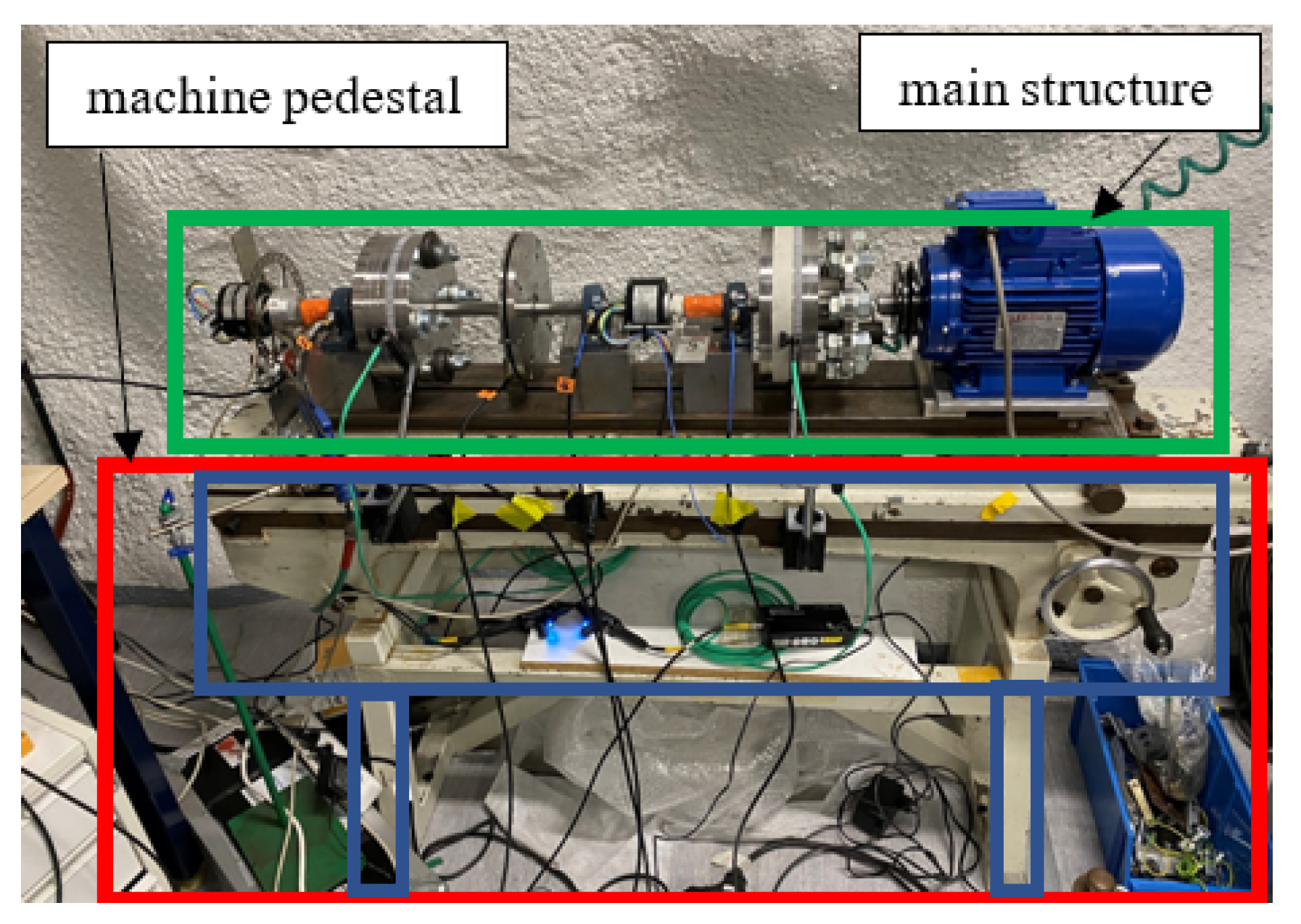
The schematic of the system is presented in Figure 2. The main structure consists of a rotor supported by four bearings. The structure is mounted on a pedestal that has a heavy mass compared to the main structure (Figure 3). This will cause the whole system to behave as a rigid body, mounted on flexible supports. The lack of information concerning the mass and stiffness properties of the machine pedestal, as well as the stiffness and damping properties of the bearings, increases the number of unknowns in the system model. The support properties and identification of $C_{Rpede}$ and $K_{Rpede}$ will be described in Section 3.3. The electric motor (Model: Kleedrive T3A 90L-6 (1.1 kW)) drives the rotor. The FE model of the rotor is built based on the CAD model of the rotor. The initial investigation and the sensitivity analysis show that, due to the high flexibility of the rubber coupling between the rotor and electric motor (Figure 4a), the motor has a low contribution to the vibration characteristic of the main rotor. Therefore, in the rotor dynamics analysis, the system is modeled as a single rotor (main rotor). However, in the equivalent model for the support, the effect of motor mass is considered. The system is supported by four ball bearings. Ball bearings 1, 3, and 4 are type UC204, and they are connected to the machine pedestal with the cubic steel blocks (Figure 4b). In the structure, disc number 2 is not a rotating part. Disc number 2 is part of the support structure, and it is attached to the machine pedestal via a plate and bolt (Figure 4c) and causes the equivalent stiffness of support 2 to be lower than other supports. Bearing 2 is a ball bearing model FAG 16004. The main dimension and material properties of the rotor are shown in

Table 1. The main dimensions and material properties of the rotor system.

Item	Value	Item	Value
Rotor diameter	20 mm	Mass of disc 1	17.22 kg
Rotor length	770 mm	Mass of disc 3	16.11 kg
Modulus of elasticity	2.05 × 1011 Pa	Mass of disc 4	3.88 kg
Poisson’s ratio	0.285	Mass of supports 1, 3, 4	8.9 kg
Density of rotor and pedestal	7850 kg/m3	Mass of support 2 (disc2)	3.54 kg

. The coupling properties are not known.

3.1. Sensor Setup

The sensor setup and instrumentation are shown in Figure 5. A total of five triaxial IEPE-type piezoelectric accelerometers were attached to the structure (Kistler 8766A050, 100 mV/g). To measure the lateral vibrations of the shaft, two (additional) accelerometers were installed into disk 2, MP7, and MP22 (Figure 6a). The angular vibration was measured by two optical tachometers from disks 1 and 3. Multi-channel signal acquisition hardware (Siemens Scadas Mobile SCM209) was used for data acquisition and signal preprocessing. A sampling frequency of 2048Hz was used for the data acquisition, which was selected to ensure that all relevant vibration components are captured during acquisition. During the analysis phase, the raw data was low-pass filtered to appropriate the frequency range. Simcenter Testlab software (formerly LMS Test.Lab) was used for measurement data post-processing, spectral analysis, order tracking, and experimental modal analysis. Simcenter Testlab is a data acquisition and analysis software for noise, vibration, and durability testing. Matlab software was used for post-processing the measured data.

In the experiments, two tests (tests-a and test-b) were performed. In these two tests, the break was physically removed from the setup. In the experiment, the initial unbalance mass and phase are not known. In test-a, the machine is running with a sweep cycle speed from 100 to 700 rpm, without additional excitation. In test-b, 99 g unbalance is added to disc 1 (by attaching a nut and bolt, Figure 6b), and the machine is accelerating with a sweep cycle speed from 200 to 700 rpm. In the calculation of the unbalance force, the speed profile ($\omega )$ is recalled from the tachometer data. The term $\mathsf{\omega }t$in Equation (7) is sensitive to the cumulative error in the measured rotating speed signal. Here, the angle $\omega t$ is updated from the collected measurement of tacho3.

3.2. Measurement Data

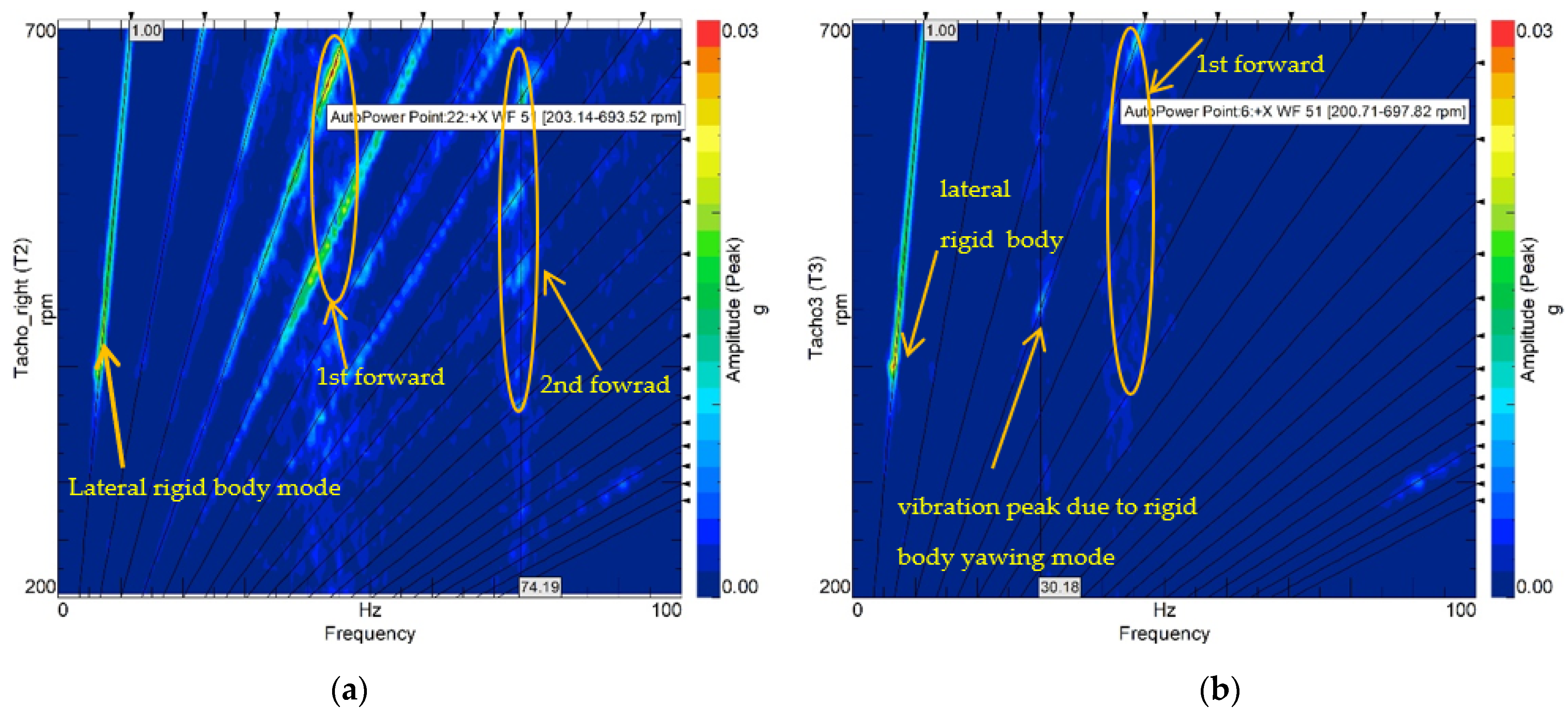
Figure 7 shows the auto-power spectral map of test-b. It can be seen in Figure 7a that for sensor MP22, in addition to the peaks at rotation speed, there are additional peaks showing the higher-order harmonic frequencies. The sensor MP22 is installed in the upper half of disc 2. This disc is connected to the machine pedestal with only one bolt, and has significantly less stiffness in comparison to the other supports, and features some directional movement. This can be a reason for the presence of higher-order harmonics. For bearings 1, 3 and 4, the higher-order frequencies are visible in the signal, but with a very low amplitude. Bearing 4 is mounted on the cubic block with a weight of 8.9 kg, and the support is stiffer compared to bearing 2. Later, the measurement data is filtered for a low-frequency range and the higher-order harmonics become insignificant, and they are beyond the scope of the simulation model.

A vibration resonance peak at 7 Hz has been observed in the measurement data for all bearings. The amplitude of vibration at this frequency in the vertical direction is significantly less than in the horizontal direction. Experimental modal analysis with impact hammer excitation was carried out to identify this frequency for the standstill rotor. The impact excitation (with hammer Endevco E2302-5) was applied to disk 4 in lateral and vertical directions (Figure 8a). The measured natural modes and natural frequencies were verified by this separate impact testing (Figure 8b). The measurement points 51–54 were located at the outer corners of the pedestal. The sensor MP33 was located on the top of the motor to identify possible motor deflection with respect to the pedestal (at higher frequencies). This sensor indicated that the motor can be considered to have a rigid connection with the pedestal. Other measuring points were located on discs 1, 2, and 3. The frequency of 7 Hz corresponds to the lateral rigid body movement of the machine pedestal. Figure 7b presents the spectral map fore sensor MP6 (at bearing 1). The resonance at 30 Hz corresponds to the rigid body yawing mode of the machine pedestal. However, this resonance cannot be seen significantly at other measuring points. The resonance at 74 Hz corresponds 2nd forward whirling mode of the rotor.

3.3. Support Identification

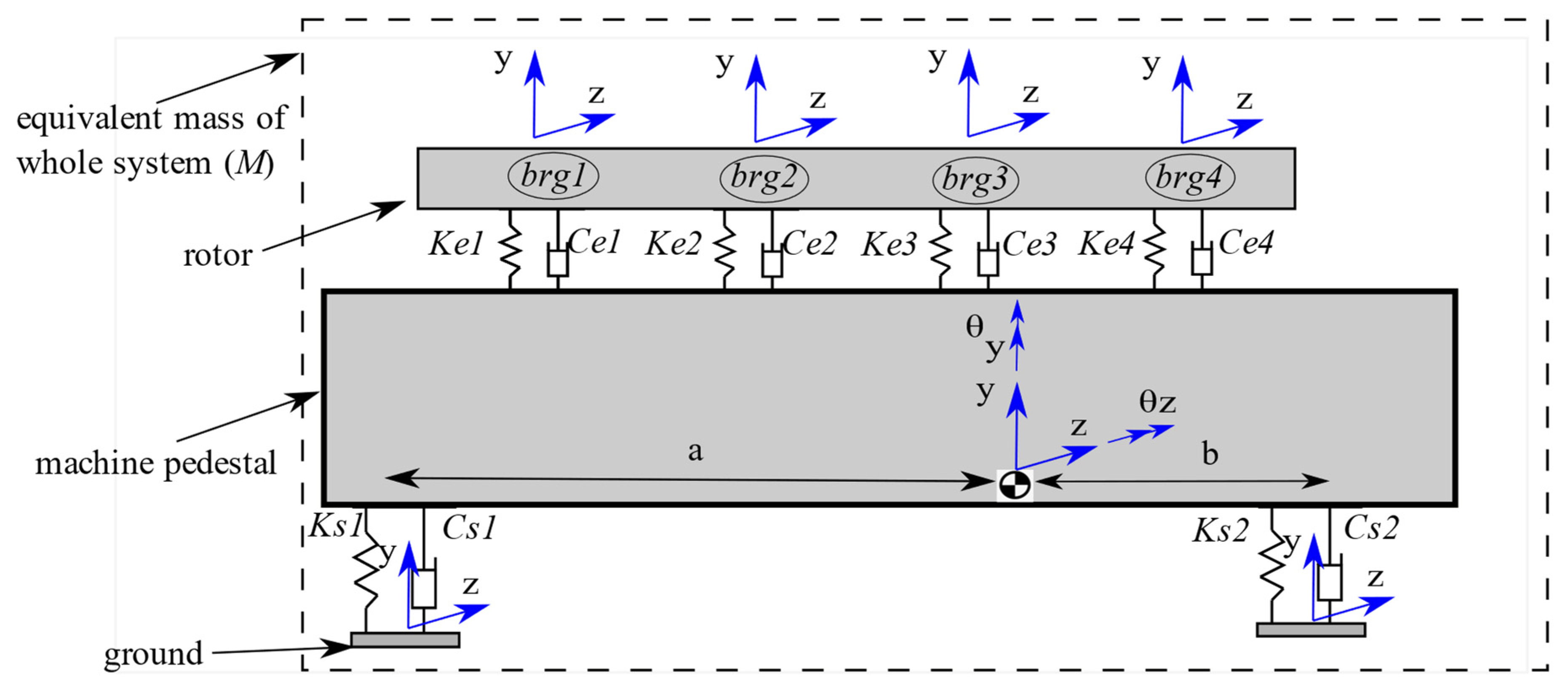
To estimate the stiffness properties of the pedestal, the support model is simplified, as shown in Figure 9, where $M$ shows the equivalent mass of the combination of the rotor, bearing blocks, electric motor, and machine pedestal. In the equivalent system, the translational and rotational motion should be included. Here, $K{s}_{1-2}$, and $C{s}_{1-2}$ show the stiffness and damping of the pedestal, respectively. The distance of the machine pedestal legs with respect to the center of the mass of the whole structure is denoted as $a$ and $b$.

Applying the simplified model, the structure movement at the center of the mass can be modeled with a single mass having four dofs. By using this model and performing the eigenvalue analysis on the equivalent mass for the whole structure and comparing the natural frequencies with the rigid body frequencies obtained from the measurement, the unknown mass properties ($M_{pede}$), and the stiffness of the machine pedestal ($K_{pede}$) can be estimated. The matrix $K_{pede}$ includes the translation and rotational stiffness and damping of the pedestal (shown by $K{s}_{1-2}$). Then, by using the proportional damping, the damping of the machine pedestal ($C_{pede}$) can be calculated.

The stiffness matrix for the machine pedestal, $K_{pede}$, has translational $(y, \mathrm{z}$) and rotational $({\theta }_y$, ${\theta }_z$) dofs and cross-coupling terms, due to the moment applied on the system (due to the unsymmetric location of the mass center). Taking into consideration the heavy mass of the pedestal and the high vertical stiffness, in Equation (8), the terms $y$ and ${\theta }_z$ for ${\mathit{q}}_{pede}$can be ignored. The combination of the ball bearing stiffness and the cubic steel blocks/disc2 forms a series spring connection, with equivalent stiffnesses denoted as $K{e}_{1-4}$. In the formation of the matrix $K_R$ and $C_R$, the stiffness and damping of the rotor, and the equivalent stiffnesses $K{e}_{1-4}$, are taken into account. The stiffness of the cubic steel is the equivalent stiffness of the bearing cap and bolt joints. It should be noted that the acceleration is measured from the bearing housing, and not directly from the shaft.

4. Results

Figure 10 shows the FE model of the rotor. The model consists of 11 elements. The bearings are modeled as spring- dampers. The bearings are located at nodes 2, 6, 7, and 8. Discs 1, 3, and 4 are modeled as a mass point at nodes 5, 9, and 12 (disc 2 does not rotate and it is part of the support). The pedestal is considered a mass point at node 13 (its location is approximated based on the center of mass of the whole structure). The free-free modes of the rotor are close to the frequencies obtained from SolidWorks model (

Table 2. Free-free modes.

Item	Simulation (Hz)	Solidworks (Hz)
Torsional	36.14	36.57
Lateral	44.61	45.15
Lateral	45.58	45.56
Lateral	84.95	88.83
Lateral	86.80	89.34

). The stiffness of the ball bearings is 1.4×10⁸ N/m and is selected based on literature [24].

The stiffness of the cubic blocks under the bearings, the connection of disc number 2 to the pedestal, and the pedestal itself are tuned based on the measurement data, as explained in Section 3.3. The system dynamics are verified using the modal analysis results. The identified support properties are shown in

Table 3. Estimated support properties.

Location	Value
stiffness $K{e}_1$ (nodes 2 to 13), (Figure 9)	1 × 108 N/m
stiffness $K{e}_2$ (nodes 6 to13)	9 × 105 N/m
stiffness $K{e}_3$ (nodes 7 to13)	1 × 108 N/m
stiffness $K{e}_4$ (nodes 8 to13)	1.1 × 108 N/m
machine pedestal stiffness-z direction (node 13 to ground)	4.6 × 105 N/m
whole mass of the structure	366 kg
inertia of the whole system	Iy = 62.12 kg m2, Iz = 8.84 kg m2

and are based on the simplified model presented earlier. Due to the connection type of support 2 (see Figure 4c), the stiffness is lower compared to supports 1, 3, and 4. The proportional damping 2 × 10⁻⁵ × bearing stiffness is used for estimating the damping of bearings 1–4 [25].

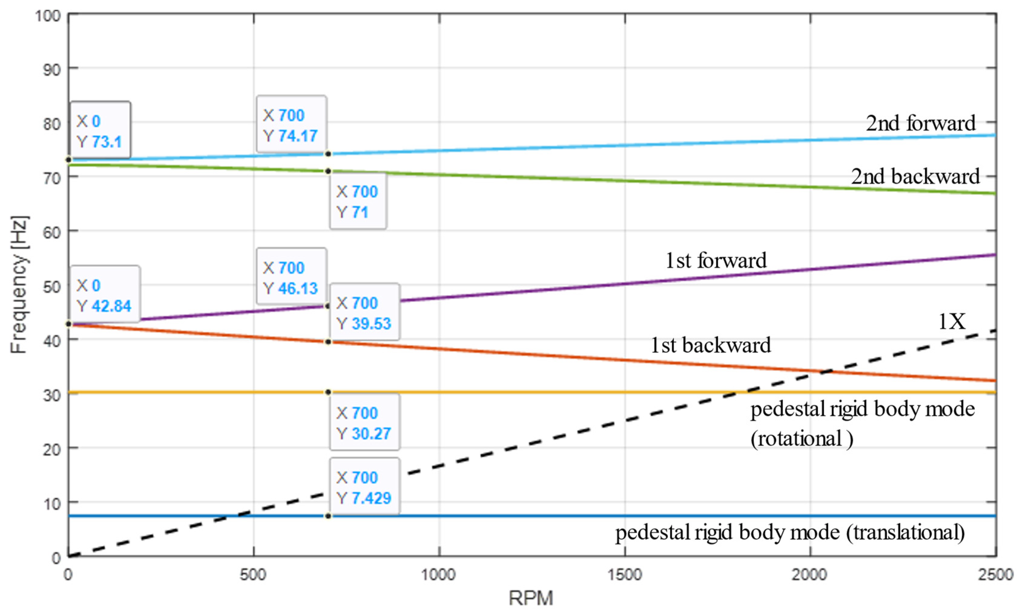
The natural frequencies obtained from the Campbell diagram (Figure 11) at 700 rpm are compared with the natural frequencies obtained from the FE model by Nastran software and the measurement data (

Table 4. Rotor and support model verification with the fem and measurement data.

	Campbell Diagram at 0 rpm	Nastran FEM at 0 rpm	Campbell Diagram at 700 rpm	Measurement at 700 rpm
torsional	36.10 (Hz)	35.15 (Hz)	36.10 (Hz)	-
1st forward	43.92 (Hz)	43.17 (Hz)	46.87 (Hz)	45.45 (Hz) at Disc344.36 (Hz) at Disc2
2nd forward	73.52 (Hz)	70.22 (Hz)	74.83 (Hz)	74.35 (Hz) at Disc2

). In the Campbell diagram, the rigid body modes, due to the machine pedestal, can be seen at 7.15 Hz and 29.92 Hz; this has good agreement with the lateral and rotational rigid body frequencies obtained from measurement (7 Hz for translational, 30 Hz for yaw movement around the y-axis). The calculated natural frequencies and mode shapes were verified by separate impact testing for the standstill rotor, as explained earlier. For the lateral rigid body mode, a damping ratio of 3.2% is obtained from the measurement.

4.1. Unbalance Response

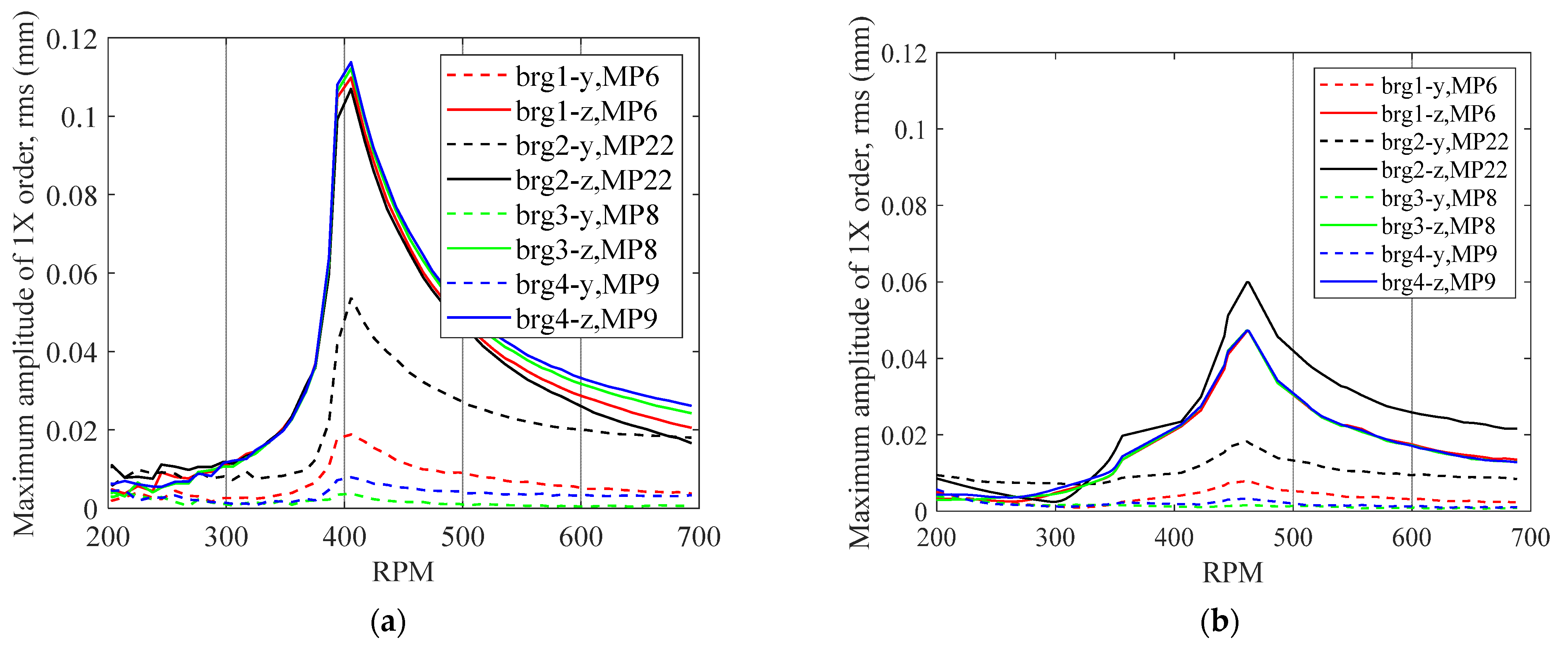
The unbalance can be recognized by a vibration peak at 1X vibration (once per revolution). In the experiment, the contribution of the pedestal movement, higher-order frequencies, and support types influence the recorded vibration measurement. Therefore, using the raw measurement data to study the unbalance response might not provide clear information concerning the system behavior. The order tracking is applied, and the first order component of the acceleration sensor data is extracted. Figure 12 shows the 1X component of the measurement data. The first order component of the measurement data is converted to mm units in order to compare it with the corresponding results from the simulation model.

Figure 12b shows the peak of the vibration at the first order, the 1X component of test-b appears at 400 rpm. The rotating speed in the case of test-a has been changed very quickly and has large fluctuation; the peak is visible at a slightly higher speed of 450 rpm (Figure 12a). The peak of frequency at the 1X component of the signal is close to the pedestal movement mode (7 Hz). The unbalance response is dominated by pedestal translational mode. The vibration peak appears primarily in the horizontal, and slightly in the vertical, direction. The vertical response of sensor MP22 is rather high. This sensor is located in the upper half of disc2 (Figure 4c) and does not capture the movement of the pedestal. Sensors MP6, MP8, and MP9 record the vibration of bearings 1, 3, and 4, respectively. The pedestal has high vertical stiffness; therefore, it cannot move significantly in this direction.

Figure 12 shows that at the end of the measurement at 700 rpm there is a small difference between the amplitude of the 1X component at test-a (without additional unbalance) and test-b (99 g unbalance was added to disc1). This shows that the residual unbalance in test-a is significant compared to test-b. Equation (7) shows that for a specific speed and a certain phase, the unbalance force is proportional to the unbalance mass. The ratio of the amplitude between the two tests shows that the unbalance phase is not the same in the two tests, and the initial unbalance on test-a is high. The exact value of unbalance remains unknown.

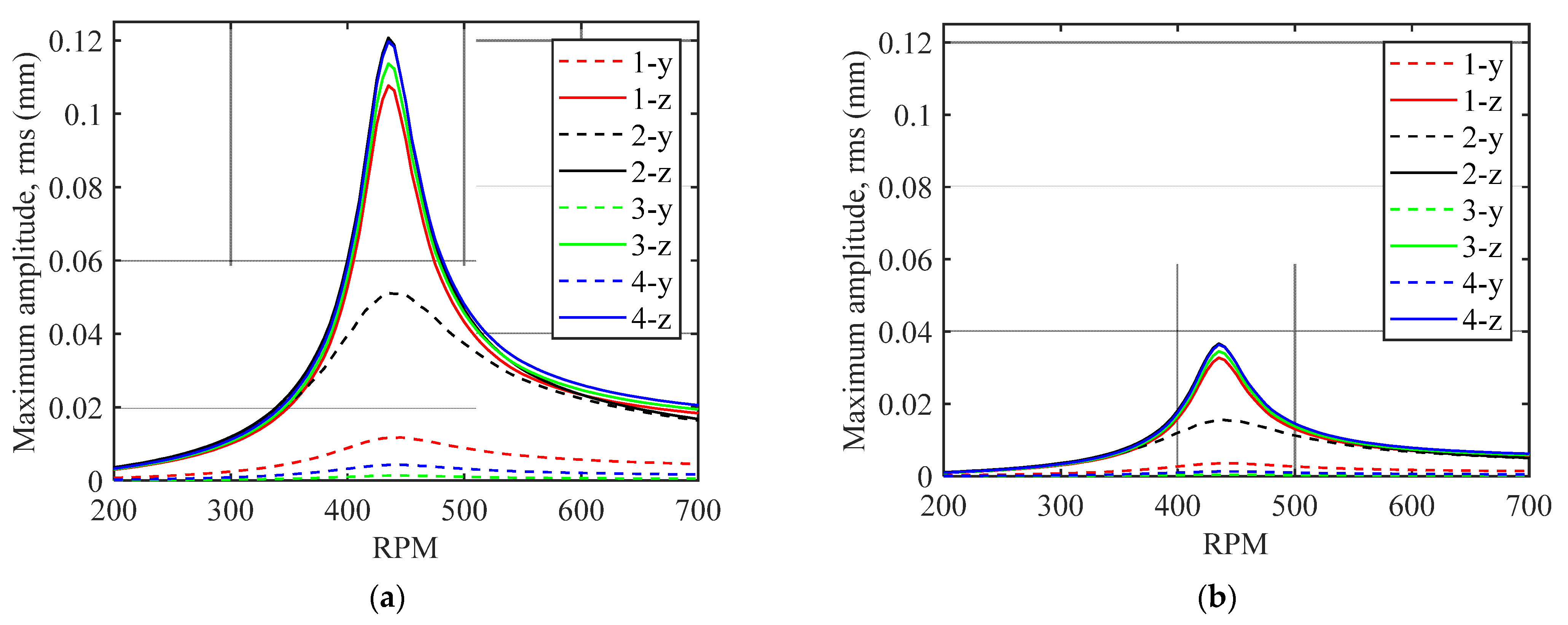
Figure 13 shows the unbalance response obtained from the simulation model. The initial unbalance and phase at test-a are not known. Therefore, it might be possible that in the setup the unbalance also exists on the other planes. In the simulation, 40 g unbalance mass is added to disc1 to provide a similar amplitude to the measurement.

4.2. State Estimation Using Kalman Filter

The Matlab ode15s integrator is used for the transient simulation of system dynamics, and it is based on the 4th order Runge-Kutta integration method for solving stiff problems. In the model, the speed profile and the sampling frequency were chosen according to the measurement data (sampling frequency 2048 Hz). The time step is 1/2048 s, the maximum integration step is 5 × 10⁻⁴ s, and the maximum allowable integration error is 1 × 10⁻⁴.

In the model, there are 150 states (3 × 50 dofs, 50 displacements, 50 velocities, and 50 acceleration). The observation is vibration recorded by the eight acceleration sensors (horizontal and vertical vibration at bearing locations). Inside the simulation model, the assumed modal reduction is used to reduce the computational time (see Appendix A). The measurement data needs to be processed before being utilized in the Kalman filter.

4.2.1. Preprocessing Measurement Data

As can be seen in Figure 14, test-a begins at 100 rpm and test-b at 200 rpm. The acceleration rates for these tests are different. At the end of the tests, the machine is running at a constant speed of 700 rpm. Figure 15a shows the raw measurement data for bearing 1, recorded in the test-b. The raw measurement data have a large variation in amplitude; it includes the higher order components, and many aspects of the model were not fully known. The low-pass filter 20 Hz was applied to the measurement data (using Simcenter Testlab software) to see a clearer image from the system behavior. This frequency range enables us to observe the main behavior of the system and remove the higher order frequencies. Figure 15b show the synchronized tachometer and acceleration for test-b. The start of the measurement data for test-a and test-b are matched in such a way that they both have the same reference point, based on the pulse recorded by tachometer. In the next section, the state estimation is carried out for the steady state part of the data.

4.2.2. Estimation of Acceleration

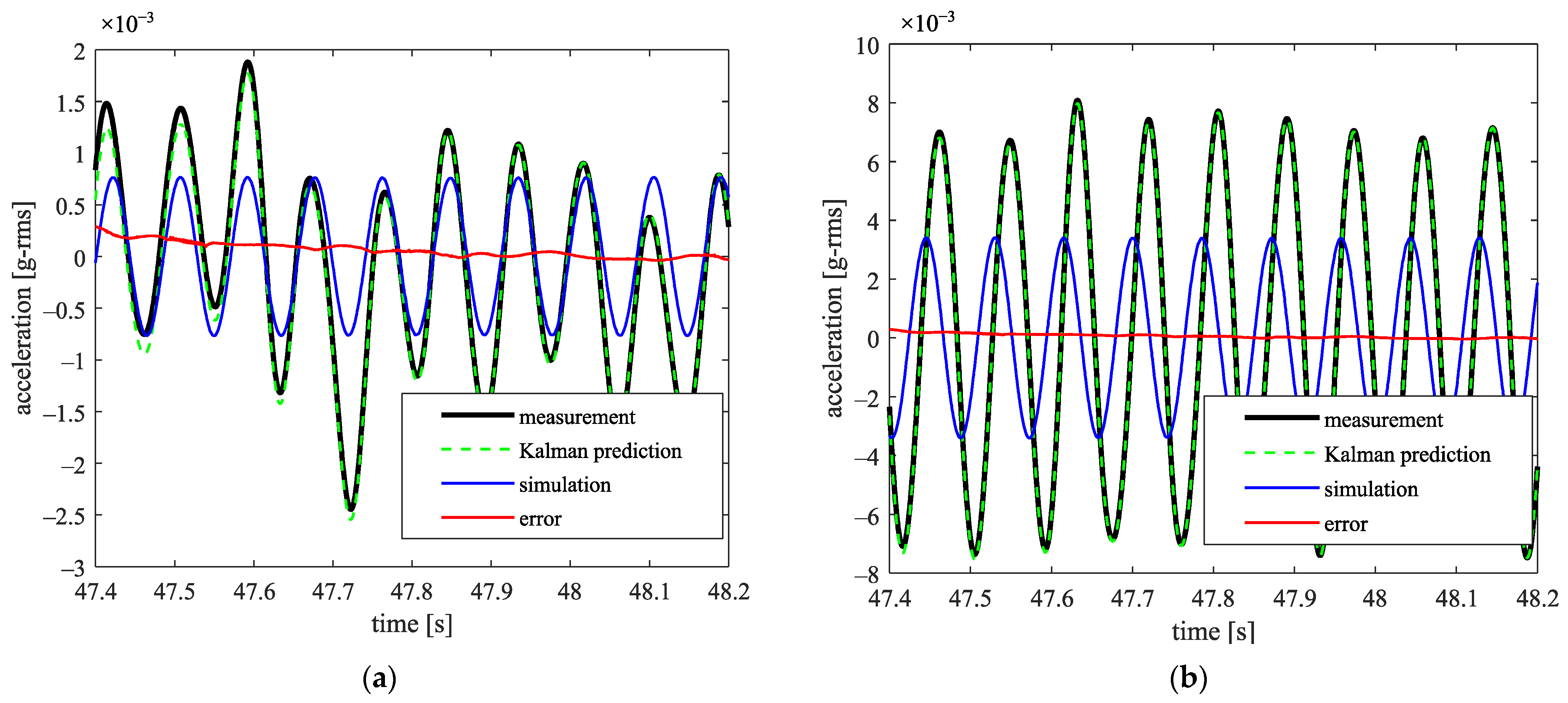
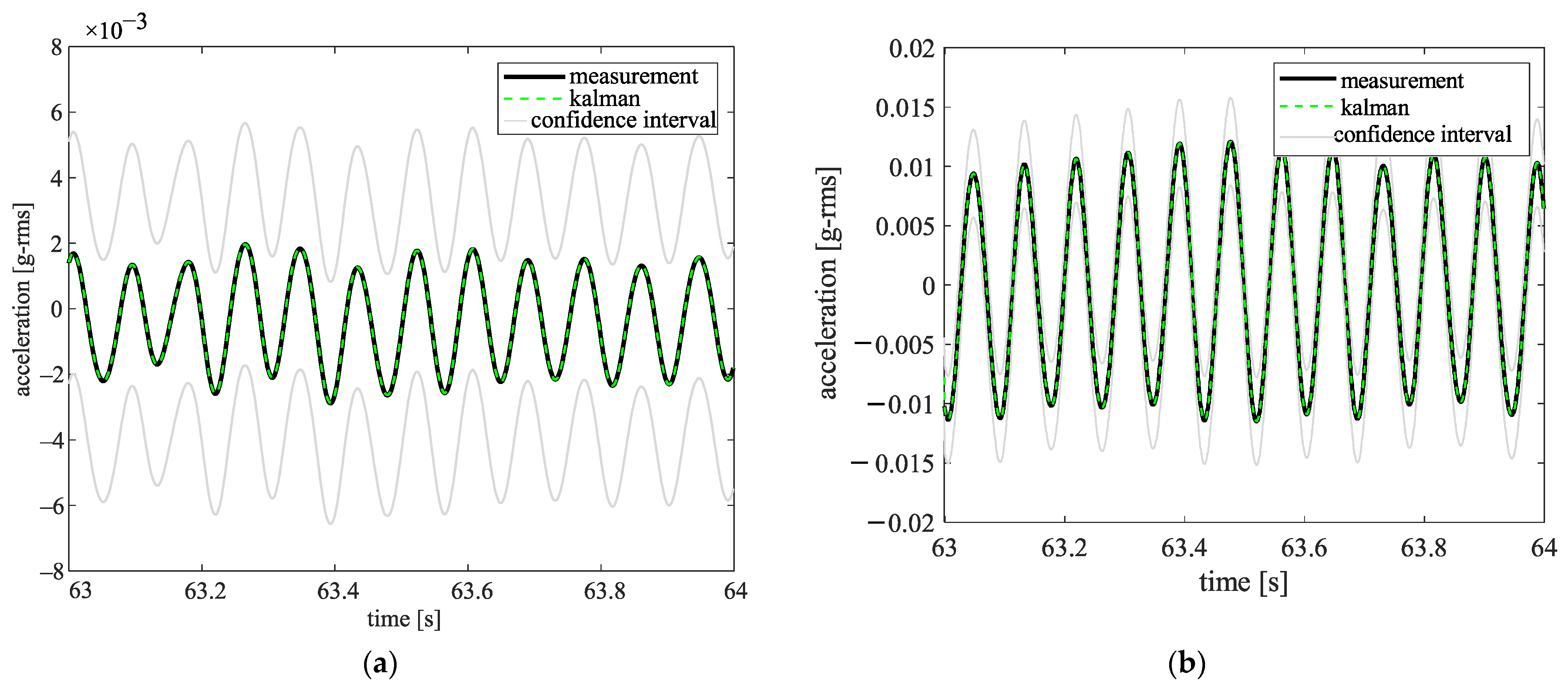
Figure 16 shows that, whilst there is a considerable difference between the simulation model and the measurement data, and all dofs are used in the model, the Kalman filter can estimate the acceleration at the bearing locations with high accuracy. The estimated value for the acceleration is within the 95% confidence interval, which has been described in detail in the study by Howard et al. [26]. The Kalman filter parameters are shown in

Table 5. Final parameter used in Kalman filter.

Item	Value
Initial covariance for simulation displacement, velocity, and acceleration	1 × 10−8, 5 × 10−8, 1 × 10−8
Process noise displacement, velocity and acceleration	1 × 10−7, 5 × 10−7, 1 × 10−7
Measurement noise level	3 × 10−6
Unscented Kalman Filter parameters ($\alpha , \beta ,\kappa )$	0.01, 2, 0
Number of states	150
Number of observations	8
Number of iterations in Kalman filter	8192
Initial states for displacement, velocity and acceleration	0

. Tuning the covariance matrix is dependent on the model and measurement data. Applying the UKF with 150 states demands a high computation burden, and it took more than eight hours to study the steady state part of the measurement data at 700 rpm. We focused on the last 4 s of measurement data (a zoom view is shown in the results). Here, the UKF is used for state estimation as it helps to consider high fluctuation in the experimental, and it was robust for this measurement.

The selection of the Kalman filter can affect computational time. The EKF uses linearization for the propagation of the error covariance matrix and Kalman gain, and it seems to be a faster solution. When the initial estimate of the state is wrong, or an accurate model is not possible to develop, the state estimation using the EKF might not converge. For problems where nonlinearity is not high, the EKF offers an acceptable performance. The UKF is more robust than the EKF and can handle high nonlinearity [27]. However, the computational effort increases due to the larger matrixes and the calculation of sigma points. In this study, after testing, it was found that the UKF is robust and can handle the raw measurement data well, while the EKF did not converge.

4.2.3. Effect of Number of Observations of the Estimation

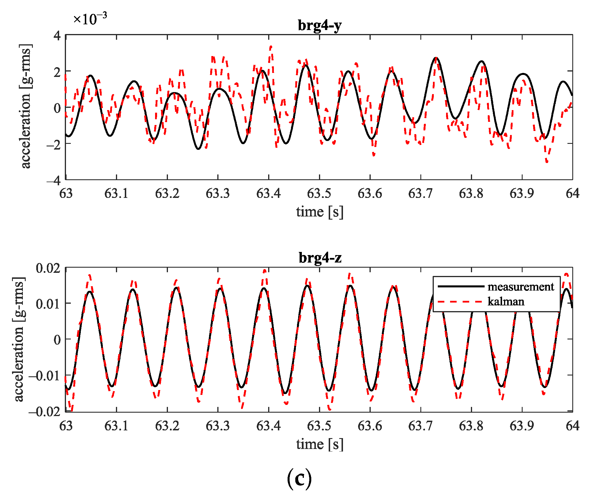
In this section, rather than presenting all eight measurement points, the measurements of three bearing locations are selected as observations, and the capability of the Kalman filter in the estimation of the response at the fourth bearing location (for validation purposes) is tested.

Table 6. Configuration used for section of observation and prediction.

Measurement	(a)	(b)	(c)
observation	brg2-y	brg1-y	brg1-y
	brg2-z	brg1-z	brg1-z
	brg3-y	brg2-y	brg2-y
	brg3-z	brg2-z	brg2-z
	brg4-y	brg4-y	brg3-y
	brg4-z	brg4-z	brg3-z
prediction	brg1-y	brg3-y	brg4-y
	brg1-z	brg3-z	brg4-z

shows the configuration for the selection of the observation and prediction points.

In Figure 17a, the measurement data at bearings 2, 3, and 4 are selected as observations and the Kalman filter is used to predict the response at bearing 1. The results are compared with the corresponding recorded measurement data. Similarly, the Kalman filter is tested for the estimation of the response at bearings 3 and 4 (Figure 17b,c). Here, bearing 2 was not chosen as a validation point because it has a different installation point for the sensor. Bearings 1, 3, and 4 have similar conditions and are more suitable for the validation. Figure 17a shows that the Kalman filter can track the measurement data at bearing 1. The estimated amplitude is close to the measurement data. There is a phase shift between the prediction response in the y-direction, which may be due to the uncertainty in the unbalance at disc 1. Figure 17b,c shows that, using the six measurement points as an observation, the Kalman filter can predict the responses at bearings 3 and 4 with reasonable accuracy. The response in the z-direction has a higher vibration due to the horizontal movement of the pedestal. The amplitude of the vibration in y-direction is relatively low.

Figure 18 shows the case in which six measurement points are used in the model (response at bearing 1, 2, and 4) and bearing 3 is used for prediction. Here, the confidence interval for the calculated response by the Kalman filter for bearing 1 is presented, showing high accuracy with respect to the measurement data, and the estimated results by the Kalman filter for the states are located within the 95% confidence interval.

4.2.4. Deflection along the Rotor

This section uses the eight measurement points of the bearing locations (nodes 2, 6, 7, and 8 of the FEM model) as an observation, and the rotor movement in all nodes are plotted in Figure 19. It can be seen from Figure 19a that the highest movement appears near discs 3 and 4 (nodes 9–12). There is a clear movement near disc 1. Discs 1, 3, and 4 are quite heavy (17.22 kg, 16.11 kg, and 3.88 kg, respectively). This caused the amplitude of the predicted acceleration at these locations to become high. In the middle of the rotor and near the bearing location, the amplitude is relatively small, as the movement is restricted.

The estimated pattern by the Kalman filter agrees reasonably well with the first forward whirling mode shape of the rotor at 700 rpm (Figure 19b), which has a significant contribution to the rotor deflection shape. It should be noted that, according to the Campbell diagram, the frequency of the first forward at 700 rpm is 46 Hz, while the 1X excitation appears at 7 Hz. The first forward mode is not the only mode contributing to the deflection at 700 rpm. In fact, the rotor deflection shape at 700 rpm is a combination of several mode shapes. The shape and magnitude of deflection is highly dependent on the amount of unbalance and its distribution, as well as the contributions of individual modes, where due to the unclear unbalance condition it cannot be investigated in detail. In the future, a detailed study into the initial unbalance, and measuring the runout in the experiment, can help to provide a clear picture of the rotor deflection. The UKF helps to deal with high uncertainty in the model, along with measurement. The main drawback of the UKF was that the computational burden took several hours, due to the large size of the matrix for the generation of sigma points. However, the UKF is not the end point for Kalman filter modeling. There are also other types of Kalman filter models. The optimum selection is dependent on the system under investigation and needs to be evaluated case by case. When the parabolic distribution has a Gaussian from, using the state-space form and the Kalman filter is suitable. During the present study, we noticed that if the parameters of the UKF, the noise covariance of the plant (Q), and measurement (R) are not selected correctly, the outlier can exist in the estimated states. In other words, there are no standard solutions or guarantees from the Kalman filter model. The nonlinear Kalman filter types also require careful tuning of the covariance and parameter selection. The stability and convergence can also be affected by the signal processing step carried out in the model. Using the proper signal processing tools, filtering the desired frequency range in advance helps to provide a more suitable data for the model. The Kalman filter is capable of considering the possible error and noise covariance in the measurement, however, we believe that, for the simple system, the UKF helps to provide a state estimation with good accuracy and predictability. The dual estimation of the UKF and EKF, the particle filter, and Kreisselmeier K-filters [28] can be also tested in the future.

5. Conclusions

This paper presents an experimental and numerical study of a rotor system with four bearings. The system under investigation resembles the typical industrial cases in which multiple unknowns exist in the system. The FE model was used for modeling the rotor. The stiffness and damping of the bearings, the support, and the pedestal were unknown, and they were approximated with the measurement data. The measurement data showed the presence of higher order harmonics and the rigid body movement of the pedestal. The impact hammer and the modal analysis of the experimental setup were carried out to find the translation and rotational rigid body movement of the frame.

In the experiments, two cases were studied: first, a system with no added unbalance; then, the single unbalance mass was added to a disc, and the vibration at the bearing locations during the sweep was measured using acceleration sensors. The initial unbalance mass and phase were not known. The first order tracking of the measurement data shows a significant initial unbalance in the system. The comparison of the unbalance response with the first-order tracking of the measurement data was used for verifying the model. The model can capture the measurement response with reasonable accuracy.

This paper also demonstrated the application of the Kalman filter for the estimation of unmeasurable parts of the machine. The UKF was used to estimate the state of the system, i.e., the displacement, velocity, and acceleration at all degrees of freedom of the FE model. To verify the results, the acceleration estimated by the Kalman filter was compared with the corresponding measurement data. The UKF algorithm can estimate the acceleration at the bearing locations with high accuracy using either eight or six measured accelerations as observations. The estimated value for the acceleration is within the 95% confidence interval.

The optimum selection of the Kalman filter model is highly dependent on the system under investigation and the measurement data, and these need to be evaluated case by case. In addition, the importance of the signal processing for identifying the main frequency and behavior of the system cannot be neglected. As the raw measurement signal might contain noise, higher order frequencies may not be of interest. The higher order frequencies can be the result of several factors, e.g., looseness, misalignment, bearing problems, etc. In the future, by modifying the support structure, improving the connection to the ground, and performing a misalignment check, the problem of possible looseness in the support can be improved, and this can help to overcome the higher order frequencies that appeared in the measurement. The present study can provide an insight into simplifying most of the real-life industrial problems in rotating machines. In addition, future research scope would aim for the optimization of the data acquisition system with open-source, cost-effective, and robust systems as, with the Kalman filter, the data quality can be compromised. Despite the limited measurement data, the system dynamics and states can be estimated.

Then, Equation (1) can be rewritten as follows:

$$M_r\ddot{\mathrm{P}}+\left(C_r+\omega G_r\right)\dot{\mathrm{P}}+K_r\mathit{P}={\mathit{F}}_{extr}$$

(23)

where P is a vector of the modal coordinate. By using the following transformation, the physical coordinates can be converted to the modal coordinate.

$$𝐪={\mathrm{S}}_{\mathrm{r}}𝐏$$

(24)

Rather than solving the system of equation with 150 dofs in physical coordinates, the transient analysis will be solved for eight modal coordinates and after solving the system of equation, the results will be converted back to the physical coordinates.