Uncertainty Analysis of Suspension System Caused by Horizontal Misalignment and Its Suppression Method

Abstract

The suspension system of the maglev train is a complex system, which is difficult to model accurately. The horizontal misalignment between the suspension magnet and the rail is one of the common uncertainty factors in the suspension system, which will affect the suspension performance. This article focuses on this problem. Firstly, the formula of suspension force considering horizontal misalignment is derived and the results of the formula and the FEA (Finite Element Analysis) simulation is consistent. Secondly, a suspension system model considering the horizontal misalignment is established for the first time, which can effectively describe the impact of the horizontal misalignment on the suspension system. Thirdly, a controller for the suspension system is designed by using the GIMC (Generalized Internal Model Control) paradigm and how the controller can effectively suppress the uncertainty caused by the horizontal misalignment is proved theoretically for the first time. Finally, the simulation and physical experiment verify that the proposed algorithm shows excellent performance and robustness in the system.

1. Introduction

Since Herman Kemper applied for the patent of the maglev train in 1937, the development of the theory and engineering of the maglev train technology has made great progress [1,2,3]. EMS (electro-magnetic suspension) system is one of the most common suspension methods in the maglev train. In China, EMS medium-and-low-speed maglev trains have been in commercial operation [4], for example, the Beijing Line S1, the Changsha Maglev Express and the Fenghuang line. Due to the demonstrated effectiveness of these two mature commercial lines, China is building more EMS medium-and-low-speed maglev train commercial lines, such as the Qingyuan line [5]. In the development of the EMS medium-and-low-speed maglev train, the stability of the suspension system is the most concerning problem. The horizontal misalignment between the rail and the suspension magnet is one of the factors that affect the stability of the suspension system, which may occur in many cases, such as when the train runs on a curved rail, the train encounters a strong wind from its horizontal direction, and so on.

Some scholars have focused on the problem caused by the horizontal misalignment. Regarding EMS medium-and-low speed maglev train as the research object, Lu [6] deduced the suspension force formula with the influence of horizontal misalignment but did not consider the whole suspension system. Yim et al. [7] paid attention to the performance when the maglev train passes through the curve and tried to minimize the variation in the lateral gap. To this end, Yim et al. established a full vehicle, multi-body dynamic model, so that the curving performance of the maglev train with U-shaped electromagnetic suspension, which provides suspension force and guiding force, could be simulated more accurately. Han et al. [8] pointed out that when the horizontal misalignment between the suspension magnet and the rail exceeds the allowable range, the maglev train cannot maintain suspension and may even be unsafe. In order to secure the system stability and improve the curving performance of the train, Han et al. proposed to install a lateral damper between the cabin and the bogie and analyzed the influence of a crosswind as the train runs along a curve and the function of the lateral damper.

To sum up, the problem caused by horizontal misalignment has attracted the attention of scholars. However, almost all relevant studies are about the impact of horizontal misalignment on the guidance system. There is a lack of research on modeling of the suspension system with uncertainty caused by horizontal misalignment and on the proposal of the corresponding suspension control strategy. Modeling the disturbance of horizontal misalignment on the suspension system can not only increase the understanding of the suspension system, but also be helpful to design an effective control algorithm to eliminate this impact.

At present, there is no suspension control algorithm that suppresses the influence of horizontal misalignment specifically. Most of the research studies build the model of uncertainty that might exist in the suspension system in two categories: structural uncertainty and non-structural uncertainty, and adopt suitable robust control algorithms to deal with them according to the category of uncertainty [9,10,11,12,13,14]. Yu et al. [10] designed a robust controller for the permanent magnet electromagnetic hybrid suspension system based on the µ synthesis, and showed that the system has good stability and anti-interference ability through simulations and experiments. Sun et al. [13] designed an adaptive robust controller based on the Riccati method and sliding mode technology, taking into account the effects of time delay and disturbance. Simulation and experiments show that the modified controller can deal with time delay and disturbance well. Fei et al. [14] propose a robust controller based on an improved suspension force model, which ensures superior system performances despite suspension force ripple, disturbances, and uncertainties while sustaining stable suspension despite system nonlinearity.

However, for most robust controllers it is difficult to achieve the best performance in the engineering of suspension systems. This is mainly because most robust control design techniques are based on the worst case: the design of a robust controller is usually at the cost of performance. Therefore, the ideal situation is that the designed robust controller will not affect the performance of the system in the nominal case, and at the same time can enhance its robustness when the system has uncertainties. In order to overcome the conflict between system performance and robustness, Zhou et al. proposed GIMC algorithm [15]. GIMC algorithm can improve the robustness of the system on the basis of the nominal controller, which has been applied in many fields and has good performance [16,17,18,19,20,21,22]. For example, Kazuhiro Yubai et al. [16] used GIMC structure in the application of the fault of strain gauge sensor of flexible arm robot, and verified the effectiveness of the algorithm through experiments. Raisemche A et al. [18] applied the GIMC method to the induction motor speed drive of the electric vehicle powertrain with faulty speed sensors, and proved the effectiveness of this structure in the case of additive and multiplicative uncertainties through experiments. Guo Wei jie et al. [19] applied a high-performance active fault-tolerant control (AFTC) method based on GIMC and feedforward compensation to HVAC systems and achieved good control results. Mingchen Xue et al. [20] apply GIMC to the electric power steering system, which has problems in relation to the modelling of uncertain and external interference, and they make it difficult for the controller to maintain the performance of the system. Through the simulation and the hardware-in-the-loop experiment, GIMC was proved to be an effective algorithm. Wu J. [21] uses the GIMC to overcome the contradiction between performance and stability in the AFS (Active Front Steering System) control. GIMC can both ensure the stability of the AFS controller and guarantee the high performance of the AFS controller. Xie W. [22] proposed a new feedback controller architecture for linear systems with a single I/O delay in the GIMC framework. The distinguishing features of the control system architecture are high tracking performance and good external disturbance rejection, which could be done separately by a nominal Smith predictor part and a finite dimensional conditional controller. A simple experiment is illustrated and proves the effectiveness of the method. At present, there is no application of the GIMC algorithm in the suspension system of the maglev train in the available literature.

The remainder of this article is organized as follows: in Section 2, the suspension force formula considering the horizontal misalignment between the suspension magnet and the rail is derived through analytical calculation and simulated in the FEA software (ANSYS Maxwell, ©2022 Copyright ANSYS, Inc., Southpointe 2600 Ansys Drive, Canonsburg, PA 15317, USA, ANSYS, Inc.). In Section 3, the horizontal misalignment is analyzed as a certain sort of model uncertainty and the suspension system model with this uncertainty is built for the first time. In Section 4, the proposed controller is designed combined with the GIMC algorithm and original algorithm. Then the nominal stability and robust stability of the closed-loop system are proved by theoretical analysis. In Section 5, the simulation and the experiment are carried out, whose results show the effectiveness of the proposed control algorithm. Section 6 is the conclusion and prospects.

2. The Suspension Force Considering Horizontal Misalignment

In this section, the suspension force of EMS maglev train is modeled, and the influence of the horizontal misalignment between the rail and the suspension magnet on the suspension force is mainly studied and analyzed. Not only is the mathematical formula of the suspension force calculated in detail, but also the FEA simulation of the influence of the horizontal misalignment is carried out for the first time.

2.1. Theoretical Analysis

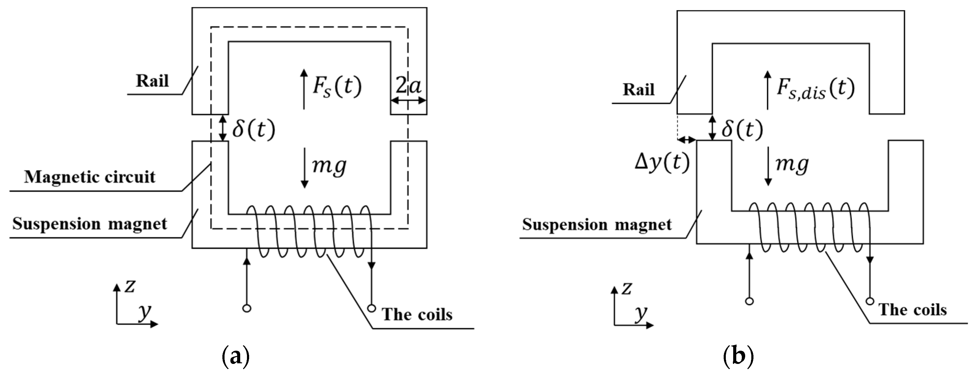
The single suspension magnet model can be regarded as the smallest model unit of the suspension system, and its basic structure is shown in Figure 1, in which, $2a$ means the width of suspension magnet, $m$ represents total mass of suspension magnet and its load, $g=9.8 \mathrm{m}·{\mathrm{s}}^{-2}$ represents the accelerate of gravity, $\delta \left(t\right)$ means the suspension gap, $∆y\left(t\right)$ means the distance of horizontal misalignment, $F_s\left(t\right)$ means the nominal suspension force, and $F_{s,dis}\left(t\right)$ means the suspension force considering the horizontal misalignment.

The nominal state of the suspension system defined in this article is shown in Figure 1a. In the nominal state, the suspension magnet and the rail do not reach magnetic saturation and there is no horizontal misalignment between them; meanwhile, the magnetic induction lines form a closed loop without leakage. According to the basic law of electromagnetic field, the expression of $F_s\left(t\right)$ is

$$F_s\left(t\right)=\frac{{\mu }_{0}S{N}_{turns}^2{I}^2\left(t\right)}{4{\delta }^2\left(t\right)}$$

(1)

where ${\mu }_0=4\pi \times {10}^{-7} \mathrm{H}/\mathrm{m}$ means permeability in vacuum, $S=2a\times L$ means the relative polar area, $L$ means the length of suspension magnet, $N_{turns}$ means turns of suspension magnet coil, and $I\left(t\right)$ means the current of the coils.

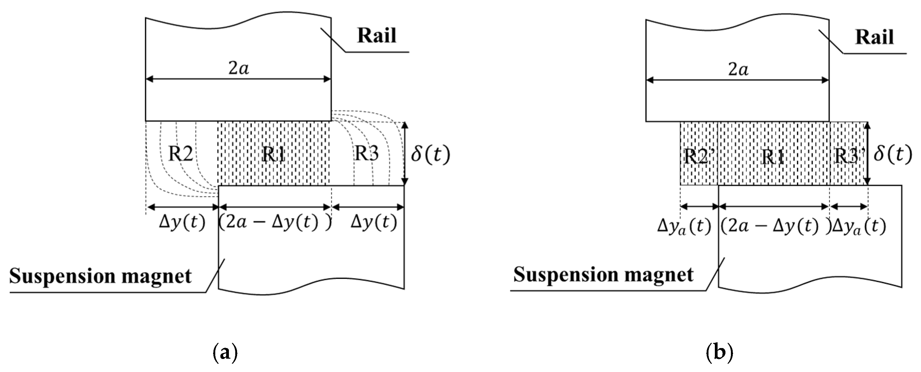
Figure 1b shows the state when the horizontal misalignment exists between the rail and the suspension magnet. When there is a horizontal misalignment, the actual distribution of magnetic induction line in the suspension gap is shown in Figure 2a. The region in the suspension gap can be divided into three parts: R1, R2, and R3.

In the region R1, the magnetic flux is considered to distribute uniformly in the suspension gap. $F_{s,R1}\left(t\right)$ means the suspension force in R1 and its expression is

$$F_{s,R1}\left(t\right)=f_{unit}\left(t\right)\cdot \left[2a-\Delta y\left(t\right)\right]$$

(2)

where $f_{unit}\left(t\right)$ means the suspension force per unit width and its expression is

$$f_{unit}\left(t\right)=\frac{{\mu }_0{N}_{turn}^2{I}^2\left(t\right)}{4{\delta }^2\left(t\right)}\frac{S}{2a}$$

(3)

In the regions R2 and R3, the distribution of magnetic flux Figure 2a can be equivalent to that shown in Figure 2b according to the literature [23]. That means the non-uniformly distributed magnetic flux in the regions R2 and R3 is equivalent to the uniformly distributed magnetic flux in the region R2′ and R3′. If $∆y_a\left(t\right)$ means the equivalent distance of horizontal misalignment, then

$$\Delta y_a\left(t\right)=\frac{\delta \left(t\right)}{\pi }+\frac{\Delta y\left(t\right)}{\pi }\arctan \left[\frac{\delta \left(t\right)}{\Delta y\left(t\right)}\right]$$

(4)

Then the expression of $F_{s,dis}\left(t\right)$ is

$$F_{s,dis}\left(t\right)=f_{unit}\left(t\right)\cdot \left[2a-\Delta y\left(t\right)+2\Delta y_a\left(t\right)\right]$$

(5)

Combine Formulas (1)–(5), then obtain

$$F_{s,dis}\left(t\right)=F_s\left(t\right)\cdot \Gamma$$

(6)

where $\Gamma$ is a variable coefficient and its expression is

$$\Gamma =1-\frac{\Delta y\left(t\right)}{2a}+\frac{\delta \left(t\right)}{a\pi }+\frac{\Delta y\left(t\right)}{a\pi }\arctan \left[\frac{\delta \left(t\right)}{\Delta y\left(t\right)}\right]$$

(7)

Let $F_{s,dis,∆y=0}$ be the suspension force amplitude when $∆y\left(t\right)=0$; then, you can obtain

$$F_{s,dis,\Delta y=0}=F_s\left(t\right)\cdot \left[1+\frac{\delta \left(t\right)}{a\pi }\right]$$

(8)

2.2. Simulation Verification

In this section, the FEA software ANSYS Maxwell (©2022 Copyright ANSYS, Inc, Southpointe 2600 Ansys Drive, Canonsburg, PA 15317 USA, ANSYS, Inc.) is used to analyze the electromagnetic field distribution and the suspension force of suspension system [24,25,26]; the detailed operation process is as follows:

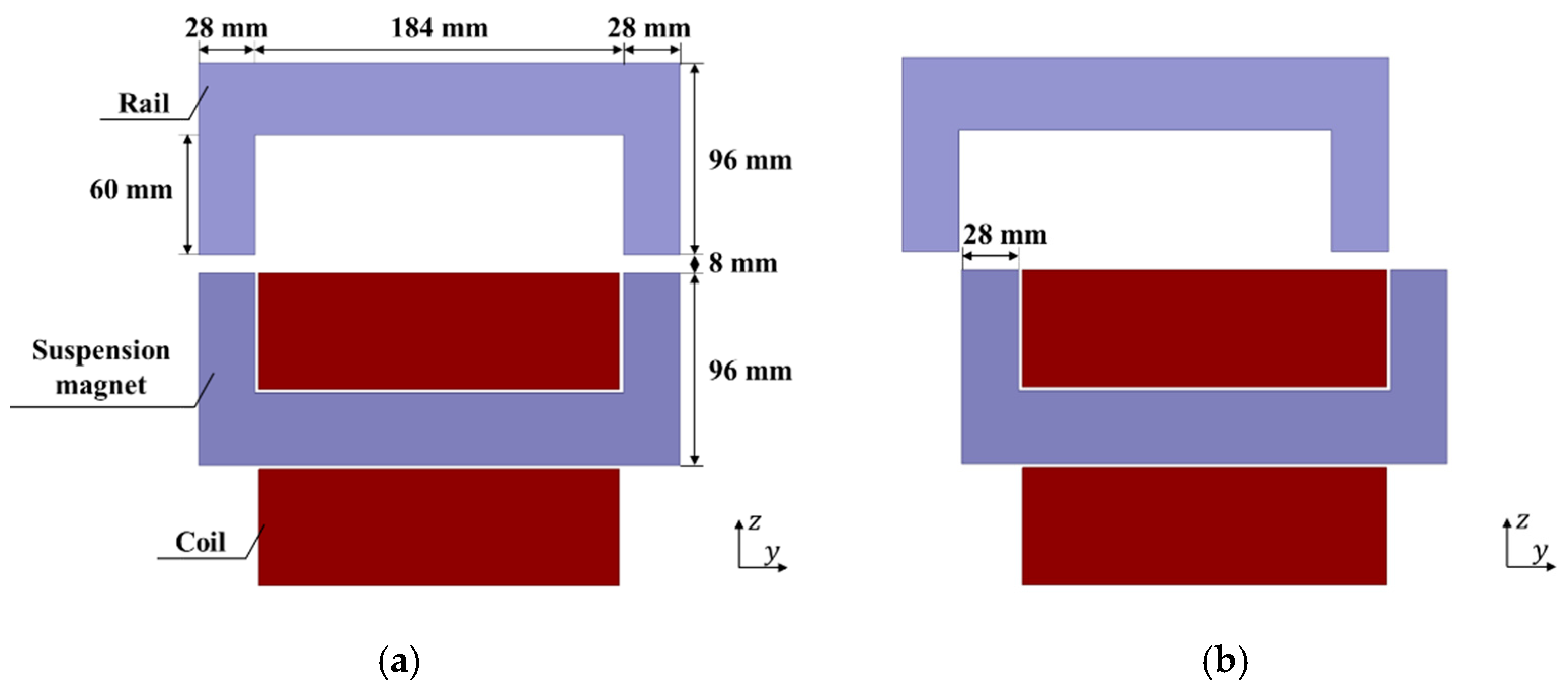
First, build a two-dimensional model as shown in Figure 3 in MAXWELL, and set the parameters according to physical size of the single bogie model. The number of coil turns of the suspension magnet is $N_{turns}=$ 360, and assume that the suspension gap and suspension current are constants, and set $\delta \left(t\right)={\delta }_0 =$ 0.008 m, $I\left(t\right) = I_0 =$ 35 A.

Then, keep the rail fixed and move the suspension magnet along the positive direction of the y axis. The simulation is carried out every 1 mm of translation until the offset is 28 mm. A total of 29 times of simulations are carried out. Figure 3a is the model diagram of the first time simulation, and $∆y\left(t\right)=0$; Figure 3b is the model diagram of the 29th time simulation, and $∆y\left(t\right)=2a=$ 28 mm.

Finally, the magnetic field distribution and the suspension force can be observed through the options of “fields” and “results → solution data” in MAXWELL.

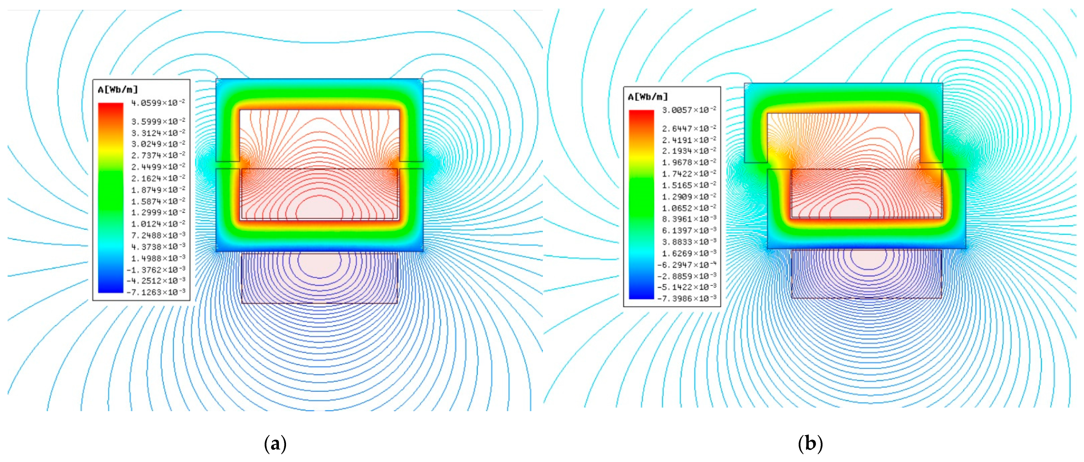
Figure 4 shows the distribution of magnetic induction lines in the conditions of $∆y\left(t\right)=0$ and $∆y\left(t\right)=2a$. The results show that when $∆y\left(t\right)=0$, the magnetic flux is basically distributed in the iron core, the rail, and the air gap between iron core and the rail, the surrounding magnetic leakage is little; when $∆y\left(t\right)=2a$, the horizontal misalignment between the suspension magnet and the rail leads to the increase of magnetic leakage and the weakening of the magnetic lines distributed in the rail.

Table 1. The simulation results of the suspension force amplitude.

$\mathbf{∆}\mathit{y}\left(\mathit{t}\right) \left[\mathbf{mm}\right]$	${\mathit{F}}_{\mathit{s},\mathit{d}\mathit{i}\mathit{s}} \left[\mathbf{N}\right]$	$\mathbf{∆}\mathit{y}\left(\mathit{t}\right) \left[\mathbf{mm}\right]$	${\mathit{F}}_{\mathit{s},\mathit{d}\mathit{i}\mathit{s}} \left[\mathbf{N}\right]$
1	16,805	15	12,415
2	16,707	16	11,969
3	16,552	17	11,509
4	16,349	18	11,036
5	16,102	19	10,557
6	15,825	20	10,062
7	15,516	21	9558.2
8	15,183	22	9042.4
9	14,831	23	8517.2
10	14,466	24	7988.5
11	14,081	25	7456.3
12	13,683	26	6925.6
13	13,275	27	6402.4
14	12,848	28	5897.2

shows the results of the suspension force amplitude in the 2nd–29th simulations. The results show that the amplitude of $F_{s,dis}$ gradually decreases with the increase of $∆y\left(t\right)$. In particular, in the first simulation, the amplitude of suspension force was $F_{s,dis,∆y=0}=$ 16,838 N.

2.3. Comparison between Formula and Simulation

Let $∆F_{s,dis,rate}$ mean the variation proportion of suspension force when horizontal misalignment exists. Its expression is

$$\Delta F_{s,dis,rate}\left(t\right)=\frac{F_{s,dis}\left(t\right)-F_{s,h,\Delta y=0}}{F_{s,dis,\Delta y=0}}\times 100$$

(9)

Combine Formulas (6), (8) and (9), when $\delta \left(t\right)={\delta }_0$, $∆F_{s,dis,rate}$ can be written as

$$\Delta F_{s,dis,rate}\left(t\right)=\frac{\left\{1-\frac{\Delta y\left(t\right)}{2a}+\frac{\delta \left(t\right)}{\pi a}+\frac{\Delta y\left(t\right)}{\pi a}\arctan \left[\frac{\delta \left(t\right)}{\Delta y\left(t\right)}\right]\right\}-\left[1+\frac{\delta \left(t\right)}{\pi a}\right]}{\left[1+\frac{\delta \left(t\right)}{\pi a}\right]}\times 100$$

(10)

In particular, $∆F_{s,dis,rate}\left(t\right)<0$ means that the suspension force is decreasing and $∆F_{s,dis,rate}\left(t\right)>0$ means that the suspension force is increasing.

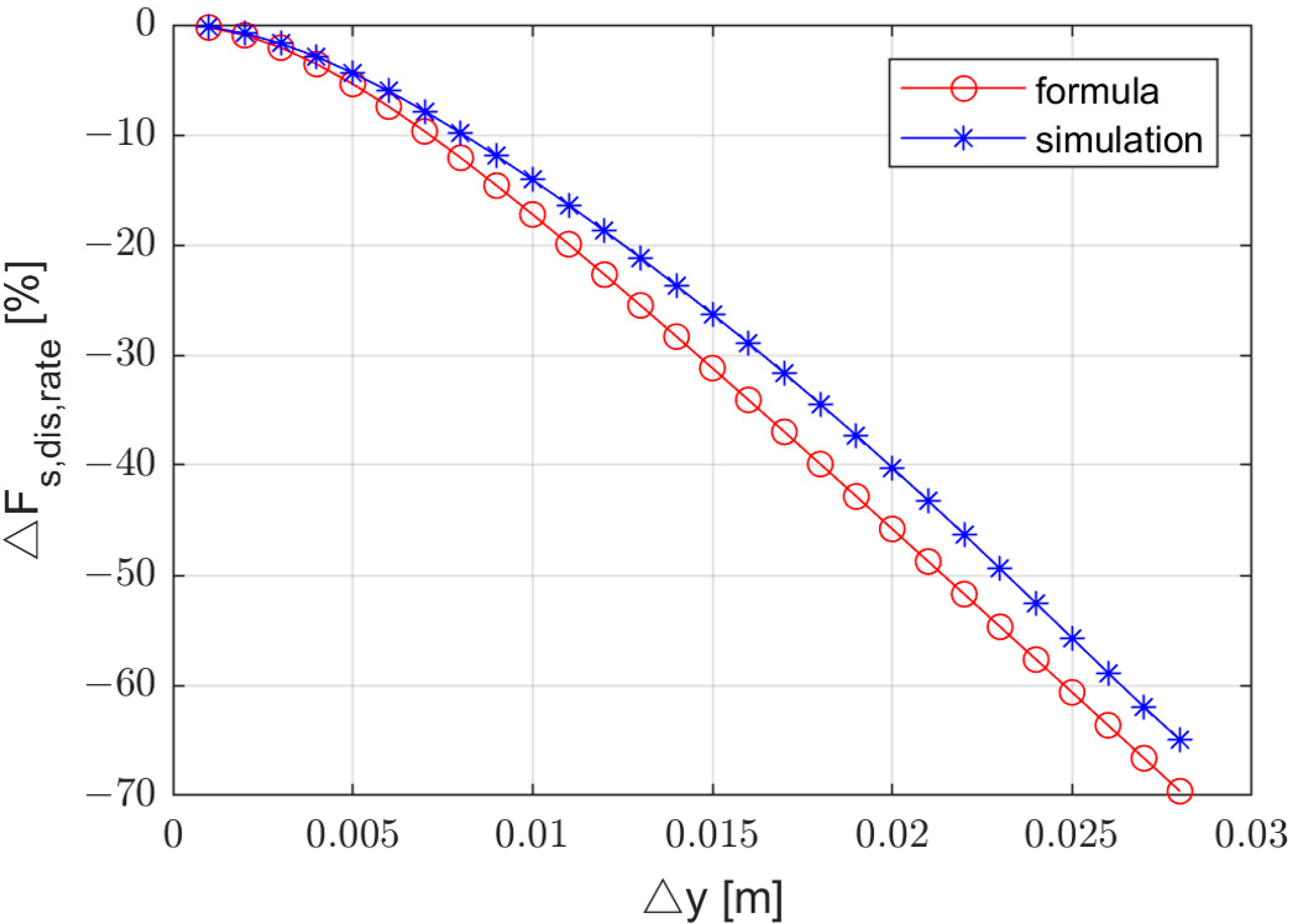
The parameters used in the simulation are substituted into Formula (10), which means $2a=$ 0.028 m, $\delta \left(t\right)={\delta }_0=$ 0.008 m, and $∆y\in$ [0, 0.028] m. Then Figure 5 can be obtained. It can be seen that, with the increase of horizontal misalignment $∆y\left(t\right),$ the amplitude of suspension force decreases. The theory and simulation results are in good agreement.

To sum up, this section deduces the suspension force formula when the horizontal misalignment exists, and analyzes the influence of the horizontal misalignment on the magnetic flux distribution and suspension force through FEA simulation for the first time, and the result of formula is in good agreement with the result of FEA simulation. The research in this section lays a foundation for modeling the suspension system.

3. System Modeling

In this section, the influence of the horizontal misalignment on the suspension system will be treated as an uncertainty for the first time, and the transfer function of the suspension system with this uncertainty is established.

3.1. The Nominal Model

To calculate the transfer function, the Taylor Formula is used to linearize Formula (1). When omitting the higher-order term, the linear nominal suspension force $F_{s,t}\left(t\right)$ is

$$F_{s,t}\left(t\right)=mg+k_I\Delta I\left(t\right)-k_{\delta }\Delta \delta \left(t\right)$$

(11)

where $∆I\left(t\right)=I\left(t\right)-I_0$ is the suspension current variation, $∆\delta \left(t\right)=\delta \left(t\right)-{\delta }_0$ is the suspension gap variation, $I_0$ and ${\delta }_0$ are the suspension current and suspension gap at the equilibrium point respectively, $k_I$ and $k_{\delta }$ are the constants and

$$k_I=\frac{{\mu }_{0}S{N}_{turn}^2{I}_0}{2{\delta }_0^2}, k_{\delta }=\frac{{\mu }_{0}S{N}_{turn}^2{I}_0^2}{2{\delta }_0^3}$$

(12)

Let $∆F_{s,dis}\left(t\right)$ mean the variation of $F_{s,t}\left(t\right)$; then,

$$\Delta F_{s,t}\left(t\right)=mg-F_{s,t}\left(t\right)=-\left[k_I\Delta I\left(t\right)-k_{\delta }\Delta \delta \left(t\right)\right]$$

(13)

According to the Newton’s second law you can obtain

$$\Delta F_{s,t}\left(t\right)=m\Delta a\left(t\right)=m\Delta \ddot{\delta }\left(t\right)$$

(14)

where $a\left(t\right)$ means the vertical acceleration of the suspension magnet and $\ddot{\delta }\left(t\right)$ means the second derivative of the suspension gap. Combine Formulas (13) and (14) and omit the incremental symbol $∆$, then you can obtain

$$m\ddot{\delta }\left(t\right)=-k_{I}I\left(t\right)+k_{\delta }\delta \left(t\right)$$

(15)

According to the relationship between current and voltage and the current loop control [27], you can obtain

$$\left[u\left(t\right)-k_{r}I\left(t\right)\right]k_0=RI\left(t\right)+L_0\dot{I}\left(t\right)-k_I\dot{\delta }\left(t\right)$$

(16)

where $\dot{\delta }\left(t\right)$ means the first derivative of the suspension gap and $\dot{I}\left(t\right)$ means the first derivative of the suspension current. In particular, $u\left(t\right)$ is the output of the controller and the input of the plant, which means it is the expected suspension current. $R$ means the resistance of the coils, $k_r$ means the feedforward coefficient of the current loop, $k_0$ means the feedback coefficient of the current loop, $L_0$ is the constant, and

$$L_0=\frac{{\mu }_{0}S{N}_{turn}^2}{2{\delta }_0}$$

(17)

Then the time-domain equations used to describe the nominal suspension system model can be written as

$$\{\begin{array}{l}m\ddot{\delta }\left(t\right)=-k_{I}I\left(t\right)+k_{\delta }\delta \left(t\right)\\ \left[u\left(t\right)-k_{r}I\left(t\right)\right]k_0=RI\left(t\right)+L_0\dot{I}\left(t\right)-k_I\dot{\delta }\left(t\right)\end{array}$$

(18)

After Laplace transformation, the frequency-domain equations used to describe the nominal suspension system model can be written as

$$\{\begin{array}{l}m\delta \left(s\right)s^2=-k_{I}I\left(s\right)+k_{\delta }\delta \left(s\right)\\ \left[u\left(s\right)-k_{r}I\left(s\right)\right]k_0=RI\left(s\right)+L_{0}I\left(s\right)s-k_I\delta \left(s\right)s\end{array}$$

(19)

Then, the transfer function from $u\left(s\right)$ to $\delta \left(s\right)$ to describe the nominal suspension system model can be obtained as

$$P_0\left(s\right)=\frac{\delta \left(s\right)}{u\left(s\right)}=-\frac{k_I{k}_0}{m{L}_0{s}^3+m\left(R+k_0{k}_r\right)s^2-k_{\delta }\left(R+k_0{k}_r\right)}$$

(20)

3.2. The Model with Uncertainty

Similarly to Section 3.1, the linear suspension force with uncertainty $F_{s,dis,t}\left(t\right)$ is

$$F_{s,dis,t}\left(t\right)=mg+k_I\Gamma \Delta I\left(t\right)-k_{\delta }\Gamma \Delta \delta \left(t\right)$$

(21)

Combine Newton’s second law when there is uncertainty:

$$m\ddot{\delta }\left(t\right)=-k_I\Gamma I\left(t\right)+k_{\delta }\Gamma \delta \left(t\right)$$

(22)

Then the time-domain equations used to describe the suspension system model with uncertainty can be written as

$$\{\begin{array}{l}m\ddot{\delta }\left(t\right)=-k_I\Gamma I\left(t\right)+k_{\delta }\Gamma \delta \left(t\right)\\ \left[u\left(t\right)-k_{r}I\left(t\right)\right]k_0=RI\left(t\right)+L_0\dot{I}\left(t\right)-k_I\dot{\delta }\left(t\right)\end{array}$$

(23)

After Laplace transforming, the frequency-domain equations used to describe the suspension system model with uncertainty can be written as

$$\{\begin{array}{l}m\delta \left(s\right)s^2=-k_I\Gamma I\left(s\right)+k_{\delta }\Gamma \delta \left(s\right)\\ \left[u\left(s\right)-k_{r}I\left(s\right)\right]k_0=RI\left(s\right)+L_{0}I\left(s\right)s-k_I\delta \left(s\right)\end{array}$$

(24)

Then, the transfer function from $u\left(s\right)$ to $\delta \left(s\right)$ to describe the suspension system model with uncertainty can be obtained as

$$P\left(s\right)=\frac{\delta \left(s\right)}{u\left(s\right)}=-\frac{\Gamma k_I{k}_0}{m{L}_0{s}^3+m\left(R+k_0{k}_r\right)s^2-\Gamma k_{\delta }\left(R+k_0{k}_r\right)}$$

(25)

It is worth noting that the uncertainty $\Gamma \in \left[{\Gamma }_{\min },{\Gamma }_{\max }\right]$ is affected by the horizontal misalignment between the suspension magnet and the rail. During the operation of the maglev train, it is difficult to obtain the value of $\Gamma$ in real time, but the range of $\Gamma$ can be calculated according to the parameters of the suspension system; that is, the value of ${\Gamma }_{\min }$ and ${\Gamma }_{\max }$.

In order to deal with this uncertainty better, let

$$\Gamma ={\Gamma }_0+{\Gamma }_w\Delta \Gamma$$

(26)

where ${\Gamma }_{\max }$ means the maximum value of $\Gamma$, ${\Gamma }_{\min }$ means the minimum value of $\Gamma$, $∆\Gamma \in \left[-1,1\right]$ is a variable coefficient, and

$${\Gamma }_0=\frac{{\Gamma }_{\max }+{\Gamma }_{\min }}{2}, {\Gamma }_w=\frac{{\Gamma }_{\max }-{\Gamma }_{\min }}{2}, \Delta \Gamma \in [-1,1]$$

(27)

Combining Formulas (25) and (26) will obtain

$$P\left(s\right)=-\frac{k_0{k}_I{\Gamma }_0+k_0{k}_I{\Gamma }_w\Delta \Gamma }{m{L}_0{s}^3+m\left(R+k_0{k}_r\right)s^2-k_{\delta }\left(R+k_0{k}_r\right){\Gamma }_0-k_{\delta }\left(R+k_0{k}_r\right){\Gamma }_w\Delta \Gamma }$$

(28)

when $∆\Gamma =1$, $\Gamma ={\Gamma }_0+{\Gamma }_{\mathrm{w}}={\Gamma }_{\max }$, it means that the horizontal misalignment is the maximum; when $∆\Gamma =-1$, $\Gamma ={\Gamma }_0-{\Gamma }_{\mathrm{w}}={\Gamma }_{\min }$, it means that the horizontal misalignment is the minimum.

4. Controller Design

The transfer function of the plant with uncertainty is built in Section 3. In this section, the controller is designed including nominal controller and robust controller, and it improves the structure of the GIMC so that it can be better applied in engineering.

4.1. The Nominal Controller

In this paper, the nominal controller is represented as $K_0\left(s\right)$, which is designed for the nominal control system. When there is no uncertainty in the plant, it is a nominal plant, and the performance of the closed-loop system with the nominal controller is called the nominal performance. The nominal performance is the ideal performance that the designer hopes the system can achieve.

The nominal controller can be designed in many ways, but the most desirable effect is that it can make the system have good nominal performance in a very simple form. As a widely used controller in engineering, PID controller is one of the most suitable choices. Therefore, this paper selects PID controller as the nominal controller.

For the plant shown in Formula (20), the nominal controller $K_0\left(s\right)$ is:

$$K_0\left(s\right)=k_P+\frac{k_i}{s}+k_{d}s$$

(29)

In which $k_p, k_i$, and $k_d$ are the proportional, integration, and differential gains, respectively. In order to $K_0\left(s\right)\in R{H}_{\infty }$, let

$$K_0\left(s\right)=\frac{k_d{s}^2+k_{p}s+k_i}{s\left(T_{d0}s+1\right)}$$

(30)

where $T_{d0}$ is a constant and $T_{d0}\ll 1$.

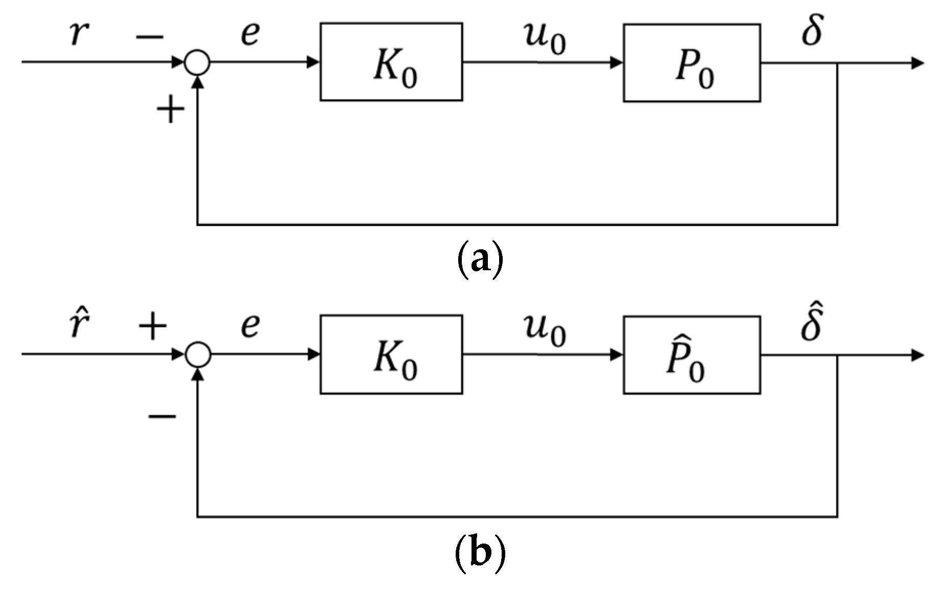
The error of the suspension system is $e=\delta -r$, so the feedback control loop composed of $K_0\left(s\right)$ and $P_0\left(s\right)$ is shown in Figure 6a, where $r$ means the desired suspension gap, $\delta$ means the actual suspension gap, and $u_0$ means the output of the controller. In order to facilitate the analysis in, the following parameters are introduced:

$$\widehat{\delta }=-\delta \begin{array}{cc},& \end{array}\stackrel{⌢}{r}=-r\begin{array}{cc},& \end{array}{\widehat{P}}_0\left(s\right)=-P_0\left(s\right)$$

(31)

It is worth noting that the closed loop transfer functions in Figure 6a,b are exactly the same, and

$$e=\delta -r=\stackrel{⌢}{r}-\widehat{\delta }$$

(32)

Therefore, in Figure 6a,b, the input and output of the nominal controller $K_0\left(s\right)$ are identical. When $K_0\left(s\right)$ is a PID controller, the gain of $k_p,k_d,k_i$ can be determined by Routh Criterion. In practical engineering, a group of appropriate gains can be selected within the range of stability conditions with the help of manual parameter tuning. Generally, the selected gain can make the system have good nominal performance. It means that under the control of the selected gain, the overshoot of the system is small, the response time is fast, and the stiffness is moderate.

4.2. The Robust Controller

When there exists uncertainties in the plant, the system can make it difficult to achieve good nominal performance under the control of the nominal controller. Under these circumstances, GIMC algorithm proposed by Zhou et al. [15] is used in the control algorithm design of the suspension system. In this section, it is proved that how the GIMC algorithm can effectively suppress the uncertainty of the numerator and denominator of the controlled object through theoretical analysis for the first time.

Combined with the basic theory of GIMC, $P\left(s\right)$ can be expressed as

$$P\left(s\right)=\frac{N(s)+W_N\Delta \Gamma }{M(s)+W_M\Delta \Gamma }$$

(33)

In which

$$W_N=-k_0{k}_I{\Gamma }_w,\begin{array}{cc}& \end{array}{W}_M=-k_{\delta }\left(R+k_0{k}_r\right){\Gamma }_w$$

(34)

$N\left(s\right),M\left(s\right)\in R{H}_{\infty }$, and $R{H}_{\infty }$ represent the set of all stable, proper, and real rational transfer functions. In order to implement the coprime factorization, ${\left(s+\theta \right)}^k$ is introduced for calculation, and $\theta$ and $k$ are the constant that make $N\left(s\right),M\left(s\right)\in R{H}_{\infty }$ true. Then

$$N\left(s\right)=\frac{-k_0{k}_I{\Gamma }_0}{{(s+\theta )}^k},\begin{array}{cc}& \end{array}M\left(s\right)=\frac{m{L}_0{s}^3+m\left(R+k_0{k}_r\right)s^2-k_{\delta }\left(R+k_0{k}_r\right){\Gamma }_0}{{(s+\theta )}^k}$$

(35)

When $k>3$, the coprime factorization condition cannot be satisfied, because there is a common zero $s=\infty$ between $N\left(s\right)$ and $M\left(s\right)$; meanwhile, when $k<3$, $M\left(s\right)$ is not proper. So that

$$k=3$$

(36)

Let $K\left(s\right)$ mean the robust controller for the plant. In order to facilitate the analysis in the following, the parameters are introduced:

$$\widehat{P}\left(s\right)=-P\left(s\right)\begin{array}{cc},& \end{array}{\widehat{W}}_M\left(s\right)=-W_M\left(s\right)\begin{array}{cc},& \end{array}\widehat{M}\left(s\right)=-M\left(s\right)$$

(37)

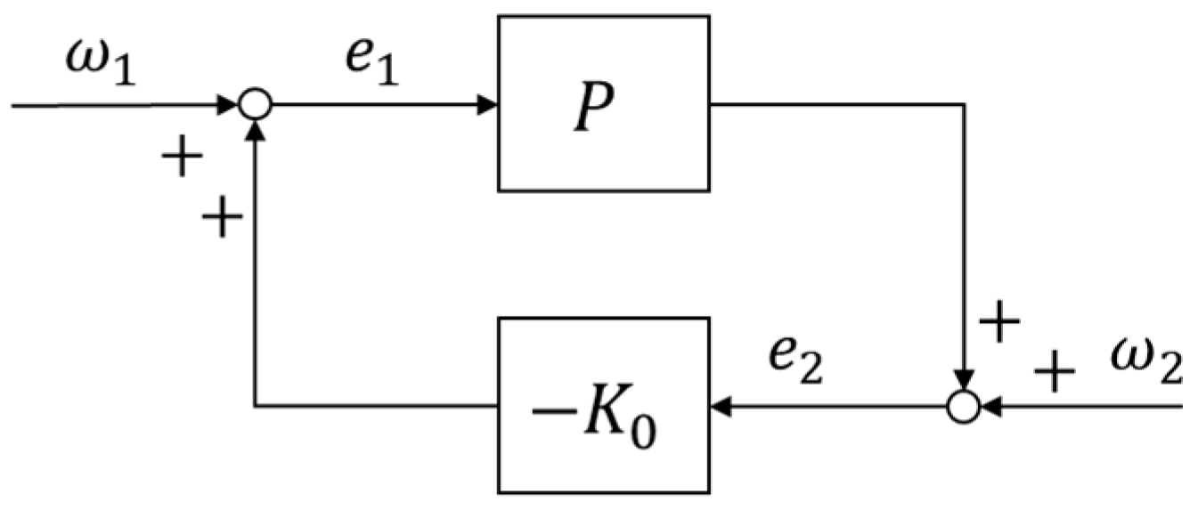
The feedback control loop composed of the controller $K\left(s\right)$ and the plant $\widehat{P}\left(s\right)$ can be obtained as shown in Figure 7.

Then, the robust controller $K\left(s\right)$ is designed. As shown in Figure 7, two concepts need to be explained:

(a)

Nominal Stability (NS): the controller $K\left(s\right)$ internally stabilizes the nominal plant ${\widehat{P}}_0\left(s\right)$.

(b)

Robust Stability (RS): the controller $K\left(s\right)$ internally stabilizes the plant $\widehat{P}\left(s\right)$.

This section will design the controller $K\left(s\right)$ that meets both NS and RS.

4.2.1. The Nominal Stability (NS)

Lemma 1.

(Youla Parameterization) [28]. Suppose that $K_0\left(s\right)$ stabilizes internally the standard feedback system shown in Figure 7. Let $K_0\left(s\right)$ and ${\widehat{P}}_0\left(s\right)$ have the coprime factorizations as $K_0\left(s\right)=V^{-1}\left(s\right)U\left(s\right)$, ${\widehat{P}}_0\left(s\right)={\widehat{M}}^{-1}\left(s\right)N\left(s\right)$. Then every controller $K\left(s\right)$ that internally stabilizes the feedback system shown in Figure 7 can be written as $K \left(s\right)={\left[V\left(s\right)-Q\left(s\right)N\left(s\right)\right]}^{-1} [U\left(s\right)+Q\left(s\right)\widehat{M}\left(s\right)]$ for some $Q\left(s\right)\in R{H}_{\infty }$ such that $\left[V (\infty )-Q(\infty )N (\infty )\right]\ne 0$.

The suspension system studied in this article is a single input single output system, so the nominal plant ${\widehat{P}}_0\left(s\right)$ can be written as

$${\widehat{P}}_0(s)=\frac{N(s)}{\widehat{M}(s)}$$

(38)

According to Lemma 1, if

$$K_0(s)=\frac{U(s)}{V(s)}$$

(39)

is a controller that can internally stabilize the nominal model ${\widehat{P}}_0\left(s\right)$, the controller $K \left(s\right)$ that meets the following formula can internally stabilize ${\widehat{P}}_0\left(s\right)$:

$$K(s)=\frac{U(s)+Q(s)\widehat{M}(s)}{V(s)-Q(s)N(s)}$$

(40)

In which, $U\left(s\right),V\left(s\right)\in R{H}_{\infty }$ is the coprime decomposition of $K_0\left(s\right)$ and satisfy.

$$N(s)U(s)+\widehat{M}(s)V(s)=1$$

(41)

Moreover, $Q\left(s\right)\in R{H}_{\infty }$ is the controller parameter that needs to be designed.

4.2.2. The Robust Stability (RS)

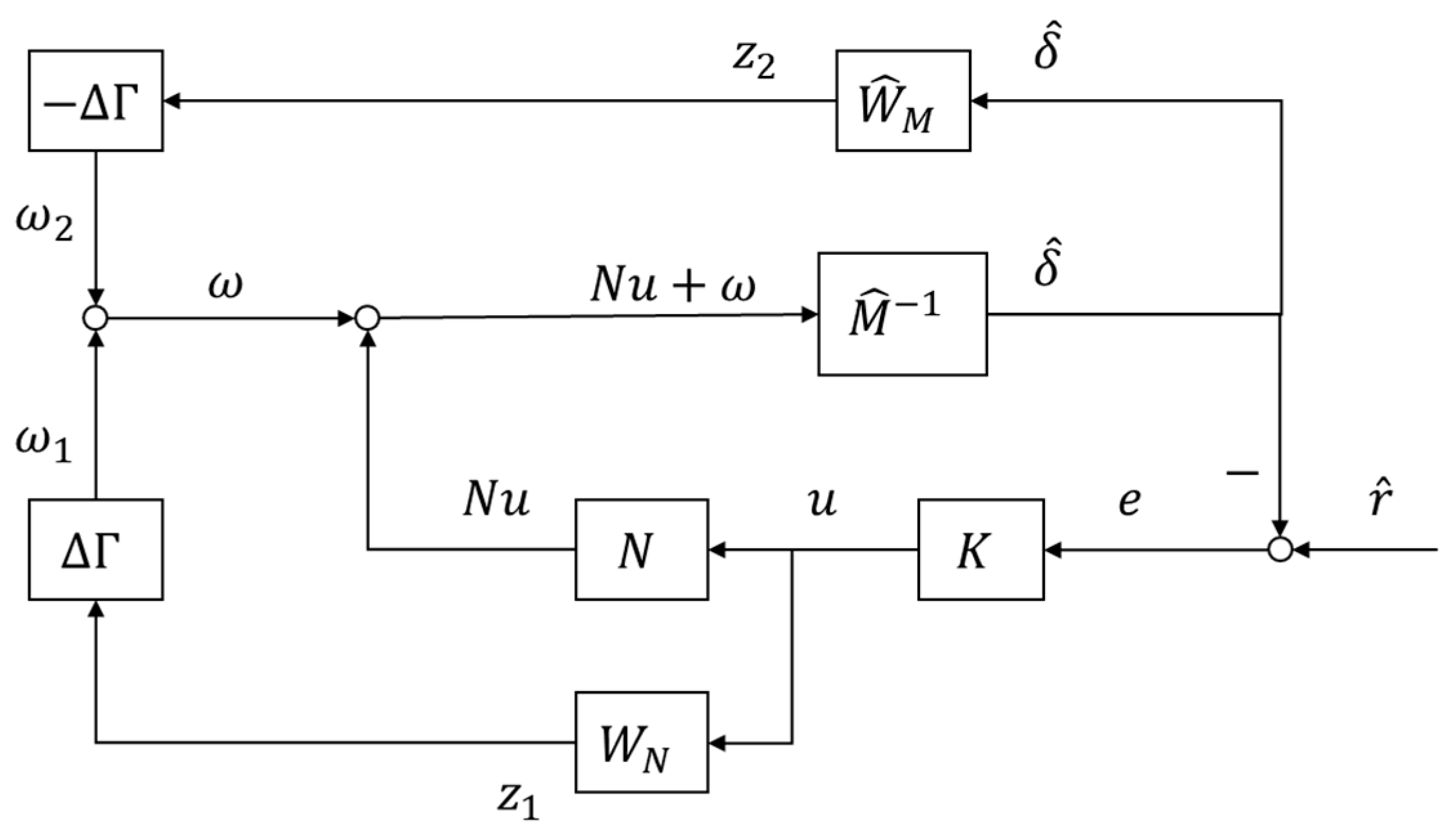
For the convenience of analysis, Figure 7 is redrawn as Figure 8 and these two figures represent the same system.

In the following analysis, the Laplace operator “s” is omitted in order to simplify the writing. Then the following formula can be obtained from Figure 8.

$$\{\begin{array}{l}e=\frac{\widehat{M}(V-QN)}{\widehat{M}V+NU}\widehat{r}-\frac{V-QN}{\widehat{M}V+NU}\omega \\ z_1=\frac{W_N\widehat{M}(U+Q\widehat{M})}{\widehat{M}V+NU}\widehat{r}-\frac{W_N(U+Q\widehat{M})}{\widehat{M}V+NU}\omega \\ z_2=\frac{{\widehat{W}}_{M}N(U+Q\widehat{M})}{\widehat{M}V+NU}\widehat{r}+\frac{{\widehat{W}}_M(V-QN)}{\widehat{M}V+NU}\omega \\ \omega =\Delta \Gamma z_1-\Delta \Gamma z_2\end{array}$$

(42)

Rewrite Formula (42) as

$$\{\begin{array}{l}\left[\begin{array}{l}e\\ z\end{array}\right]=M_{LFT}\left[\begin{array}{l}\widehat{r}\\ \omega \end{array}\right]\\ \omega =\Delta z\end{array}$$

(43)

In which

$$\begin{array}{l}z=\left[\begin{array}{l}{z}_1\\ z_2\end{array}\right],\begin{array}{cc}& \end{array}\Delta =[\Delta \Gamma ,-\Delta \Gamma ],\begin{array}{cc}& \end{array}{M}_{LFT}=[\begin{array}{l}{M}_{11}\\ M_{21}\end{array}\begin{array}{l}{M}_{12}\\ M_{22}\end{array}],\\ M_{11}=\widehat{M}(V-QN){(\widehat{M}V+NU)}^{-1},\begin{array}{c}\end{array}{M}_{12}=-\left(V-QN\right){(\widehat{M}V+NU)}^{-1},\\ M_{21}=\left[\begin{array}{l}{W}_N\widehat{M}(U+Q\widehat{M})\\ {\widehat{W}}_{M}N(U+Q\widehat{M})\end{array}\right]{(\widehat{M}V+NU)}^{-1},\begin{array}{c}\end{array}{M}_{22}=\left[\begin{array}{l}-W_N(U+Q\widehat{M})\\ {\widehat{W}}_M(V-QN)\end{array}\right]{(\widehat{M}V+NU)}^{-1}\end{array}$$

(44)

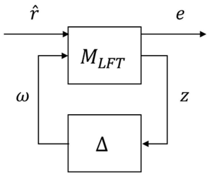
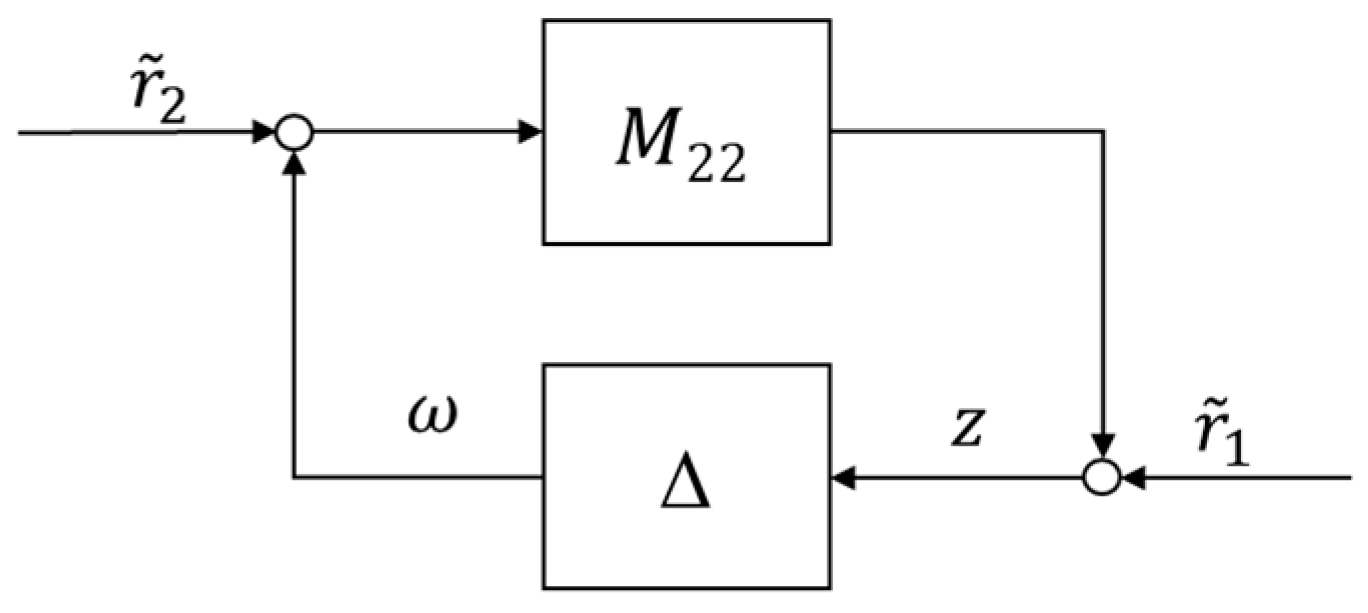
Then Figure 9 and Figure 10 can be obtained. Specially, Figure 9 is a typical LFT (Linear Fractional Transformation) analysis block diagram. In Figure 10, ${\tilde{r}}_1=M_{21}r , {\tilde{r}}_2=0$.

Lemma 2.

(Small Gain Theorem) [28]. Suppose $M_{22}\left(s\right)\in R{H}_{\infty }$ and $\gamma >0$. Then the interconnected system shown in Figure 10 is well-posed and internally stable for all $∆\left(s\right)\in R{H}_{\infty }$ with

(a). ${\Vert ∆\Vert }_{\infty }\le 1/\gamma$ if and only if $\Vert M_{22}\Vert {}_{\infty }<\gamma$;

(b). ${\Vert ∆\Vert }_{\infty }<1/\gamma$ if and only if $\Vert M_{22}\Vert {}_{\infty }\le \gamma$.

Lemma 3.

[28]. Consider the system in Figure 11, where $K_0\left(s\right)=\frac{U\left(s\right)}{V\left(s\right)}$, ${\widehat{P}}_0\left(s\right)=\frac{N\left(s\right)}{\widehat{M}\left(s\right)}$, $\left[U\left(s\right),V\left(s\right)\right]$ is a stable coprime factorization of $K_0\left(s\right)$, $[\widehat{M}\left(s\right),N\left(s\right)]$ is a stable coprime factorization of the controlled object ${\widehat{P}}_0\left(s\right)$, and $\widehat{M}\left(s\right),N\left(s\right),U\left(s\right),V\left(s\right)\in R{H}_{\infty }$. The following conditions are equivalent:

(a). The feedback system is internally stable.

(b). $\left[\widehat{M}\left(s\right)V\left(s\right)+N\left(s\right)U\left(s\right)\right]$ is invertible in $R{H}_{\infty }$.

Theorem 1.

Consider the system in Figure 7. Let $K\left(s\right)=\frac{U\left(s\right)+Q\left(s\right)\widehat{M}\left(s\right)}{V\left(s\right)-Q\left(s\right)N\left(s\right)},\widehat{P}\left(s\right)=\frac{N\left(s\right)+W_N∆\Gamma }{\widehat{M}\left(s\right)+{\widehat{W}}_M∆\Gamma }, {\widehat{P}}_0\left(s\right)=\frac{N\left(s\right)}{\widehat{M}\left(s\right)}$, and $\widehat{M}\left(s\right),N\left(s\right),U\left(s\right),V\left(s\right),Q\left(s\right)\in R{H}_{\infty }$. Assume there is uncertainty $∆=\left[∆\Gamma ,-∆\Gamma \right]\in R{H}_{\infty }$, and ${\Vert ∆\Vert }_{\infty }\le 1$. Then the closed-loop system in Figure 7 is well-posed and internally stable for all ∆ if and only if

$${\Vert \left[\begin{array}{l}-W_N(U+Q\widehat{M})\\ {\widehat{W}}_M(V-QN)\end{array}\right]{(\widehat{M}V+NU)}^{-1}\Vert }_{\infty }<1$$

(45)

Proof. 

By Lemma 3, the closed-loop system is internally stable if and only if

$${\left[\left(N+W_N\Delta \Gamma \right)\left(U+Q\widehat{M}\right)+\left(\widehat{M}+{\widehat{W}}_M\Delta \Gamma \right)\left(V-QN\right)\right]}^{-1}\in R{H}_{\infty }$$

(46)

Since $K\left(s\right)$ stabilizes ${\widehat{P}}_0\left(s\right)$,

$${\left[N\left(U+Q\widehat{M}\right)+\widehat{M}\left(V-QN\right)\right]}^{-1}\in R{H}_{\infty }$$

(47)

Then condition (46) is satisfied if and only if

$${\left[I+\frac{W_N\Delta \Gamma \left(U+\widehat{M}Q\right)+{\widehat{W}}_M\Delta \Gamma \left(V-NQ\right)}{NU+\widehat{M}V}\right]}^{-1}\in R{H}_{\infty }$$

(48)

The Formula (48) equals

$${\left[I-[\Delta \Gamma ,-\Delta \Gamma ]\left[\begin{array}{l}-W_N(U+Q\widehat{M})\\ {\widehat{W}}_M(V-QN)\end{array}\right]{(\widehat{M}V+NU)}^{-1}\right]}^{-1}\in R{H}_{\infty }$$

(49)

By Lemma 2, the above is true for all ${\Vert ∆\Vert }_{\infty }\le 1$ if and only if Formula (45) is true. □

Furthermore, according to the definition of LFT, the closed-loop transfer function from $r$ to $e$ can be calculated as

$$T_{er}=F_l(M_{LFT},\Delta )=M_{11}+M_{12}\Delta {(I-\Delta M_{22})}^{-1}{M}_{21}$$

(50)

where $M_{11}\left(s\right)$ represents the influence of reference signal $r$ on the output $e$, the rest part represents the influence of uncertainty $∆$ on the output $e$, and

$$\begin{array}{l}{M}_{12}\Delta {(I-\Delta M_{22})}^{-1}{M}_{21}\\ =\frac{-(V-QN)(U+Q\widehat{M})(\Delta \Gamma W_N\widehat{M}-\Delta \Gamma {\widehat{W}}_{M}N)}{\left(\widehat{M}V+NU\right)\left[\widehat{M}V+NU+\Delta \Gamma W_N(U+Q\widehat{M})+\Delta \Gamma {\widehat{W}}_M(V-QN)\right]}\end{array}$$

(51)

It can be seen that when

$$V-QN=0 or U+Q\widehat{M}=0$$

(52)

the influence of uncertainty $∆$ on the system is zero. Because the suspension system ${\widehat{P}}_0\left(s\right)=\frac{N\left(s\right)}{\widehat{M}\left(s\right)}$ has unstable poles, for the suspension system

$$Q=-\frac{U}{\widehat{M}}\notin R{H}_{\infty }$$

(53)

Then for the suspension system, the optimal solution of $Q\left(s\right)$ is

$$Q=\frac{V}{N}$$

(54)

4.3. The Controller Structure

The controller $K\left(s\right)$ that meets both NS and RS is designed in the previous section, and the optimal controller parameter $Q\left(s\right)$ that can eliminate the model uncertainty is obtained through theoretical analysis. This section will analyze the controller structure designed in the previous section and further improve GIMC to better apply in the engineering.

Figure 12 shows the GIMC structure and the Theorem 1 can be applied to it. It is worth emphasizing that how the GIMC algorithm can overcome the conflict between performance and robustness in the traditional feedback framework can be explained:

(a)

If the signal $f=N\left(s\right)u-\widehat{M}\left(s\right)\widehat{\delta }$ is zero when $\widehat{P}\left(s\right)={\widehat{P}}_0\left(s\right)$, then the inner loop in Figure 12 does not work. At this time, the closed-loop system has the nominal performance under the nominal controller $K_0\left(s\right)=U\left(s\right)/V\left(s\right)$.

(b)

If signal $f=N\left(s\right)u-\widehat{M}\left(s\right)\widehat{\delta }$ is NOT zero when $\widehat{P}\left(s\right)\ne {\widehat{P}}_0\left(s\right)$, that means the inner loop is active when there is a model uncertainty or other sources of uncertainties such as disturbances and sensor noises. Therefore, the robustness of the closed-loop system can be enhanced with the help of the inner loop.

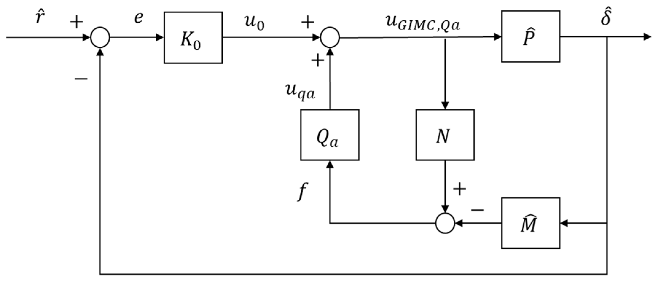
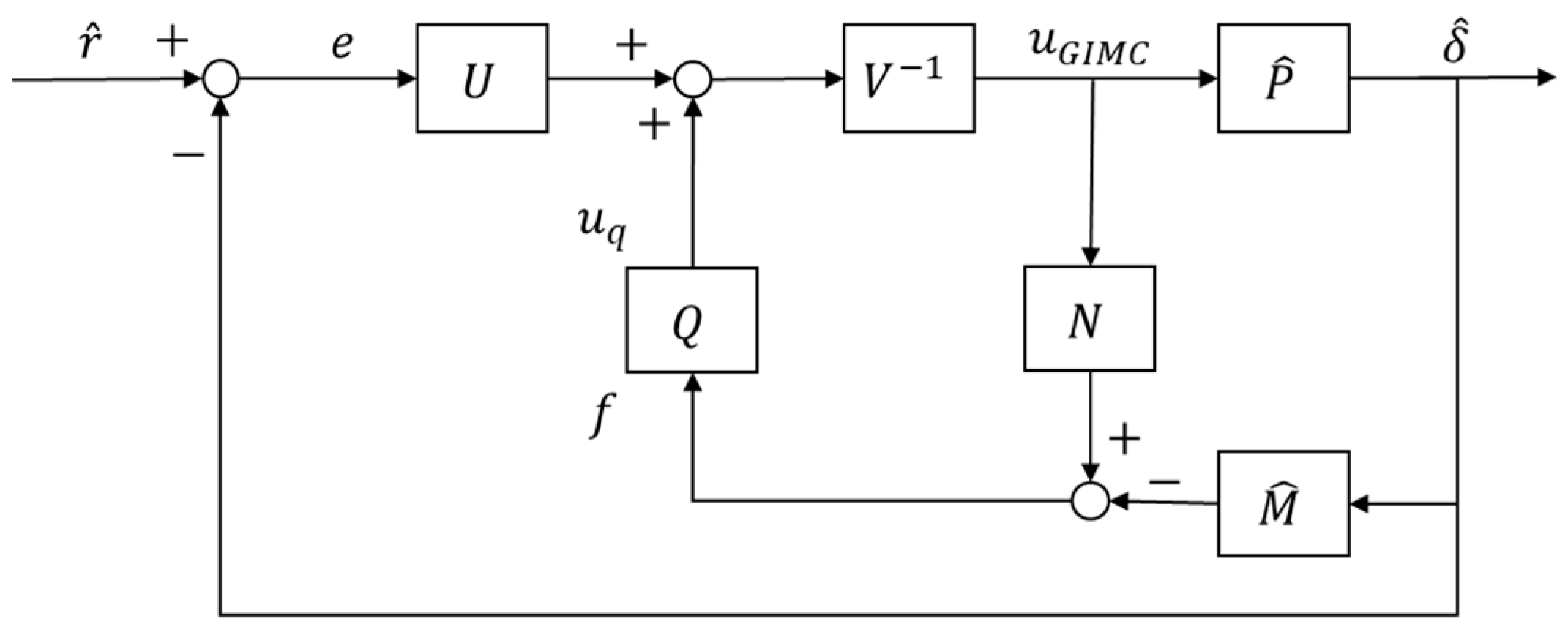
According to the previous analysis, Figure 12 has an obvious disadvantage, which is that, when $K_0\left(s\right)$ is PID controller, the coprime decomposition will not only introduce new parameters, but also not be conducive to engineering application, so Figure 12 is optimized to Figure 13 in this article.

Figure 12. The standard GIMC control structure for the suspension system.

Figure 12. The standard GIMC control structure for the suspension system.

For Figure 12,

$$u_{GIMC}=\frac{U}{V-QN}\widehat{r}-\frac{U+Q\widehat{M}}{V-QN}\widehat{\delta }$$

(55)

For Figure 13,

$$u_{GIMC,Qa}=\frac{K_0}{1-Q_{a}N}\widehat{r}-\frac{K_0+Q_a\widehat{M}}{1-Q_{a}N}\widehat{\delta }=\frac{U}{V-Q_{a}VN}\widehat{r}-\frac{U+Q_{a}V\widehat{M}}{V-Q_{a}VN}\widehat{\delta }$$

(56)

It can be seen that Formula (55) equals Formula (56) if and only if

$$Q=Q_{a}V$$

(57)

From Formula (57), it can be obtained that

$$Q_a=\frac{1}{N}$$

(58)

5. Simulation and Experiment

The previous analysis shows that the horizontal misalignment will cause the uncertainty of the numerator and denominator of the suspension system, and the GIMC control algorithm can effectively suppress this uncertainty. This section will verify this through simulation and experiments.

In this section, the proposed control structure used in simulations and experiments is carried out according to Figure 13. When setting $Q_a\left(s\right)$ according to Formula (58), to ensure that $Q_a\left(s\right)\in R{H}_{\infty }$, let

$$Q_a=\frac{1}{N}=\frac{{(s+\theta )}^k}{-k_0{k}_I{\Gamma }_0{(Ts+\theta )}^k}$$

(59)

where k$=3,$ $T=1/100$. In addition, due to the special structure of the GIMC block diagram, the value of $\theta$ will not affect the system performance. It is worth noting that in Figure 13, in the case of $Q_a\left(s\right)=0$, the plant was only controlled by the PID feedback controller. Therefore, the simulation and experiment in this section are divided into two groups for comparison. Only the values of $Q_a\left(s\right)$ in the control group are different, and the other settings are the same. The first group is in the case of $Q_a\left(s\right)=0$, the simulation or experiment under the “PID control algorithm” hereinafter. The second group selects $Q_a\left(s\right)$ as Formula (59), which will be referred to as the simulation or experiment under “GIMC control algorithm” later.

$K_0\left(s\right)$ is PID feedback controller, the selection of the values of $k_p,k_i,k_d$ is according to theoretical calculation and engineering practice. These parameters can make the system reach the critical damping state in theory, and have achieved good performances in engineering. Specifically, under the control of these parameters, the suspension system has small overshoot, fast response time, moderate stiffness, and small fluctuation of the suspension gap.

The analysis in this section will depend on two experimental platforms:

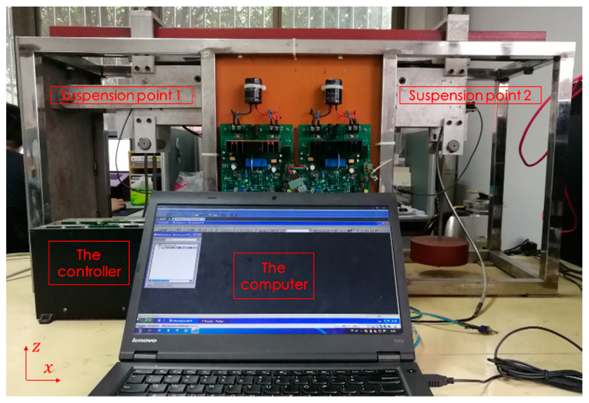
One is the small-scale experimental platform of the suspension system, as shown in Figure 14. The suspension principle of this platform is completely consistent with the suspension system of the maglev train; the main difference is smaller size and no secondary system. The parameters of the plant are based on the blueprint of the small scale experimental platform, as shown in

Table 2. Relevant parameters of the suspension system.

Symbols	The Small-Scale Platform	The Single Bogie Platform
$2a$	0.01 m	0.028 m
$L$	0.014 m	0.66 m
$S$	0.0014 m2	0.01848 m2
$m$	46.69 kg	250 kg
$N_{turns}$	663	360
$R$	2 Ω	0.55 Ω
${\delta }_0$	0.0065 m	0.008 m
$k_0$	200	250
$∆y$	[0, 0.001] m	[0, 0.028] m
$\Gamma$	[0.7807, 1.4138]	[0.3591, 1.1819]
${\Gamma }_0$	1.0973	0.7705
${\Gamma }_{\mathrm{w}}$	0.3165	0.4114

.

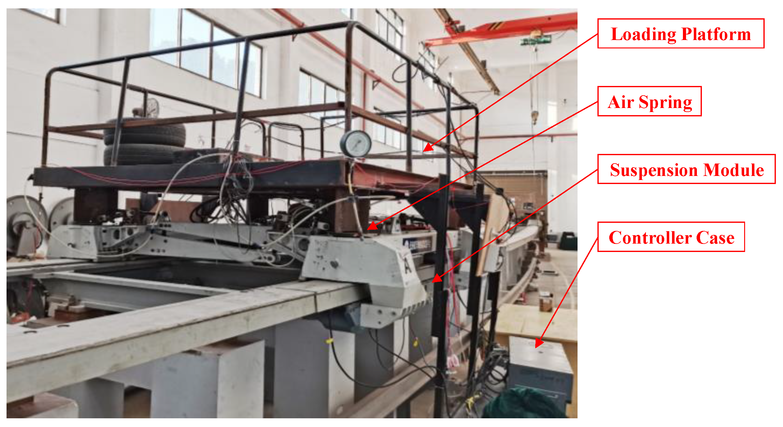
The other one is the single bogie experimental platform of the suspension system, as shown in Figure 15, which shows a single bogie experimental platform of the maglev train whose structure and size are completely the same as the maglev train that runs in commercial lines. In the project, five single bogies carry a carriage of a maglev train. A single bogie test platform mainly includes a loading platform, an air spring, a suspension module and a controller. The parameters of the plant are based on the blueprint of the experimental platform, as shown in Table 2.

5.1. Simulation Analysis

In this section, Figure 13 and Figure 14 will be simulated in the MATLAB software (MATLAB R2021a, Natick, Apple Hill Campus, MA, USA, MathWorks Inc.).

Simulation 1:

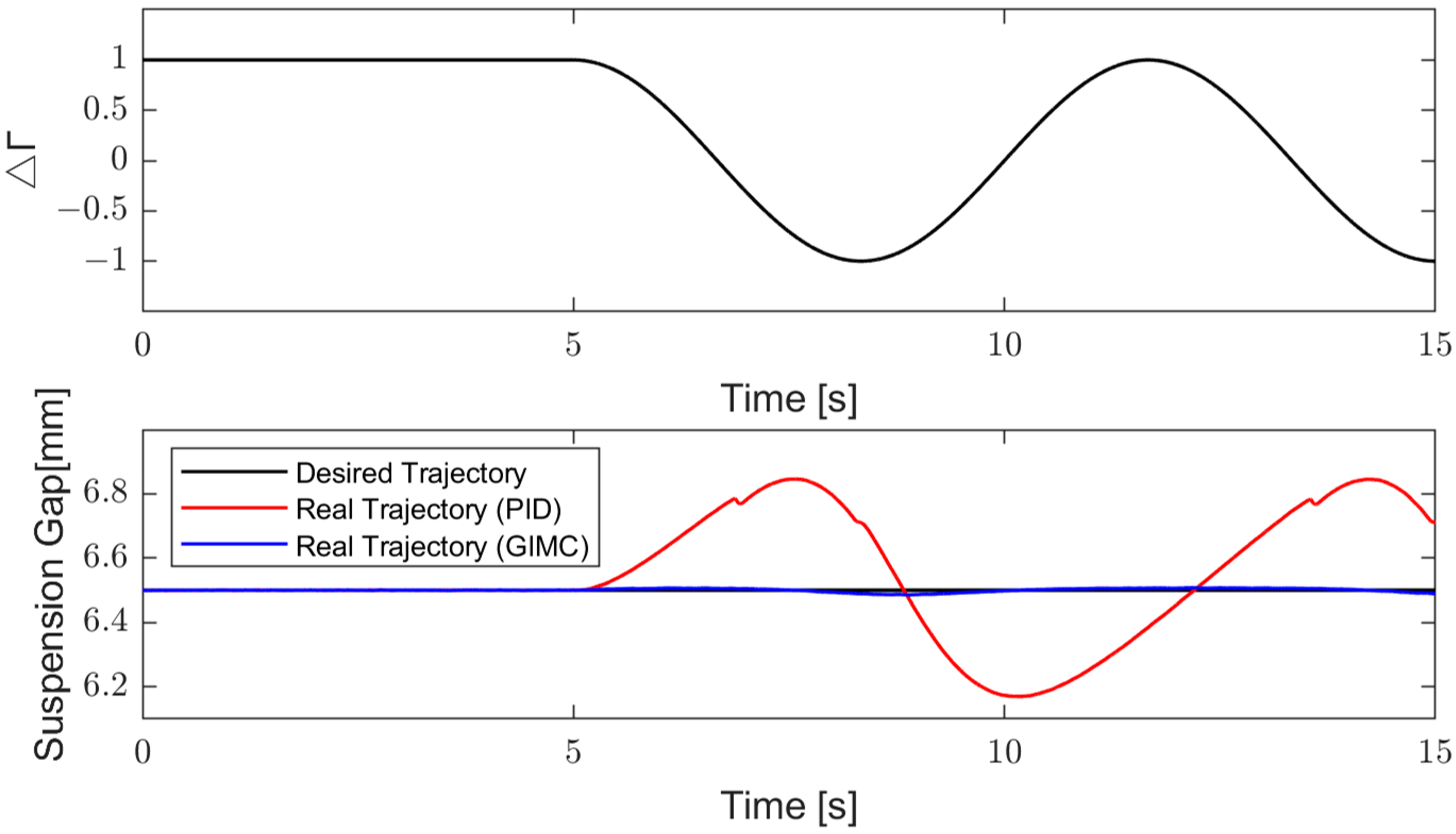
Make the system suspend stably at 0.0065 m. Then make $∆\Gamma$ change sinusoidally in the interval of $\left[-1,1\right]$, which can simulate the situation when the train runs on the curved rail. The simulation results are shown in Figure 16.

The figure shows the variation of $∆\Gamma$ with time. At 0–5 s, $∆\Gamma =1$, it means that there is no horizontal uncertainty in the suspension system; at 5–15 s, $∆\Gamma$ changes sinusoidally with time, with an amplitude of 1 and a frequency of 0.15 Hz. The desired trajectory is 0.0065 m over the whole course.

It can be seen that with the control of the PID algorithm, the fluctuation of the actual suspension gap is quite obvious; under the control of GIMC algorithm, the suspension gap is always very close to 0.0065 m, which is hardly affected by the change of $∆\Gamma$.

Simulation 2:

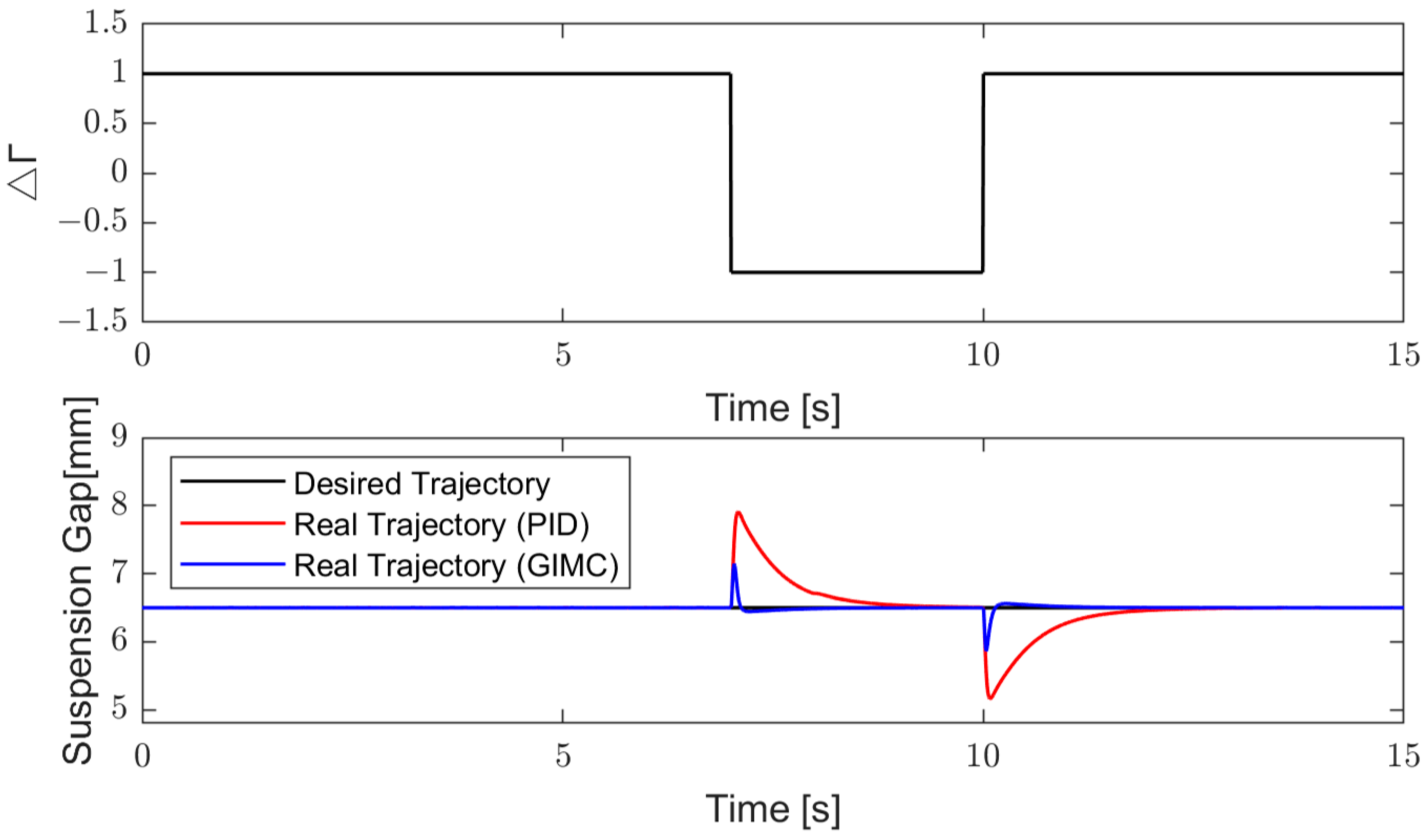
Make the system firstly suspend stably at 0.0065 m. Let the value of $∆\Gamma$ change to $-1$ at 7 s, then let the value of $∆\Gamma$ change to $1$ at 10 s. This can simulate the situation when the train encounters strong lateral wind during driving. The simulation results are shown in Figure 17.

The figure shows the variation of $∆\Gamma$ with time. When $∆\Gamma =-1$, the misalignment between the suspension magnet and the rail of the suspension system reaches maximum. The whole course of desired trajectory is 0.0065 m.

It can be seen that under the control of GIMC algorithm, the fluctuation of the suspension gap is significantly reduced and the adjustment time is obviously faster.

5.2. Experiment in the Small-Scale Experimental Platform

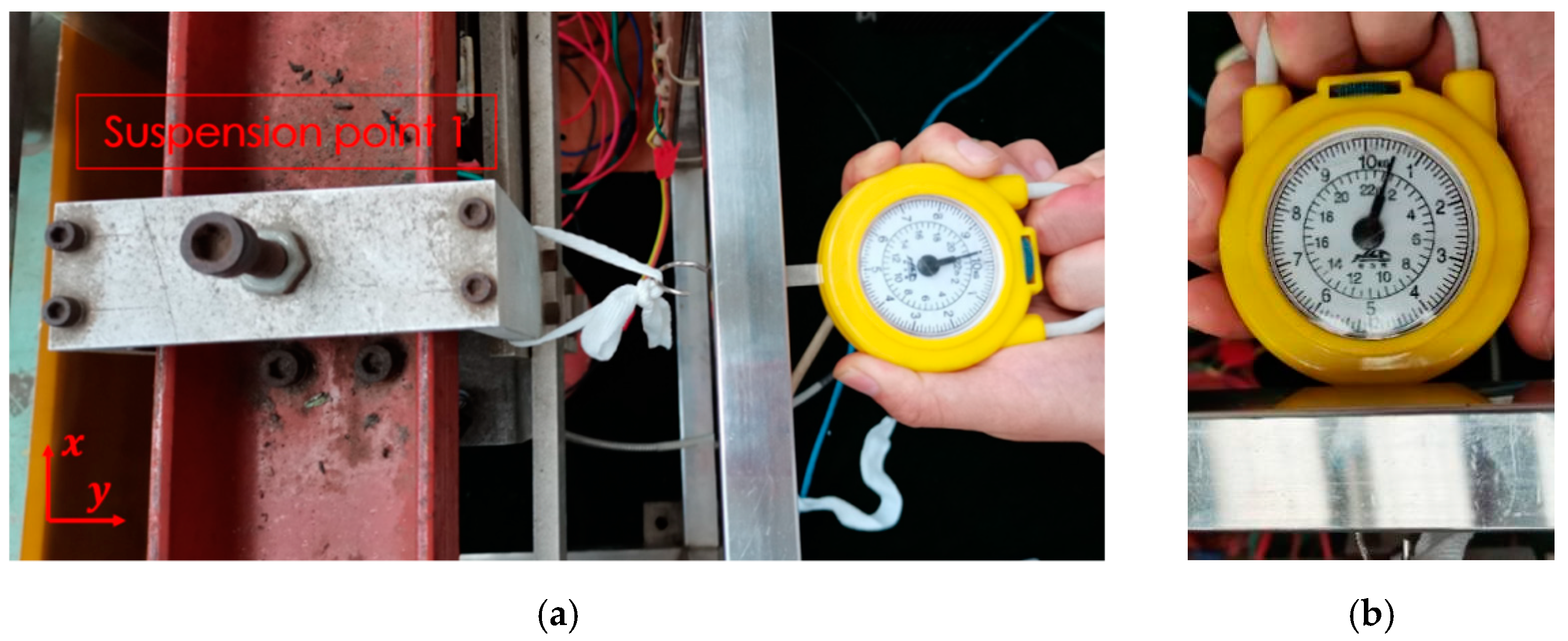
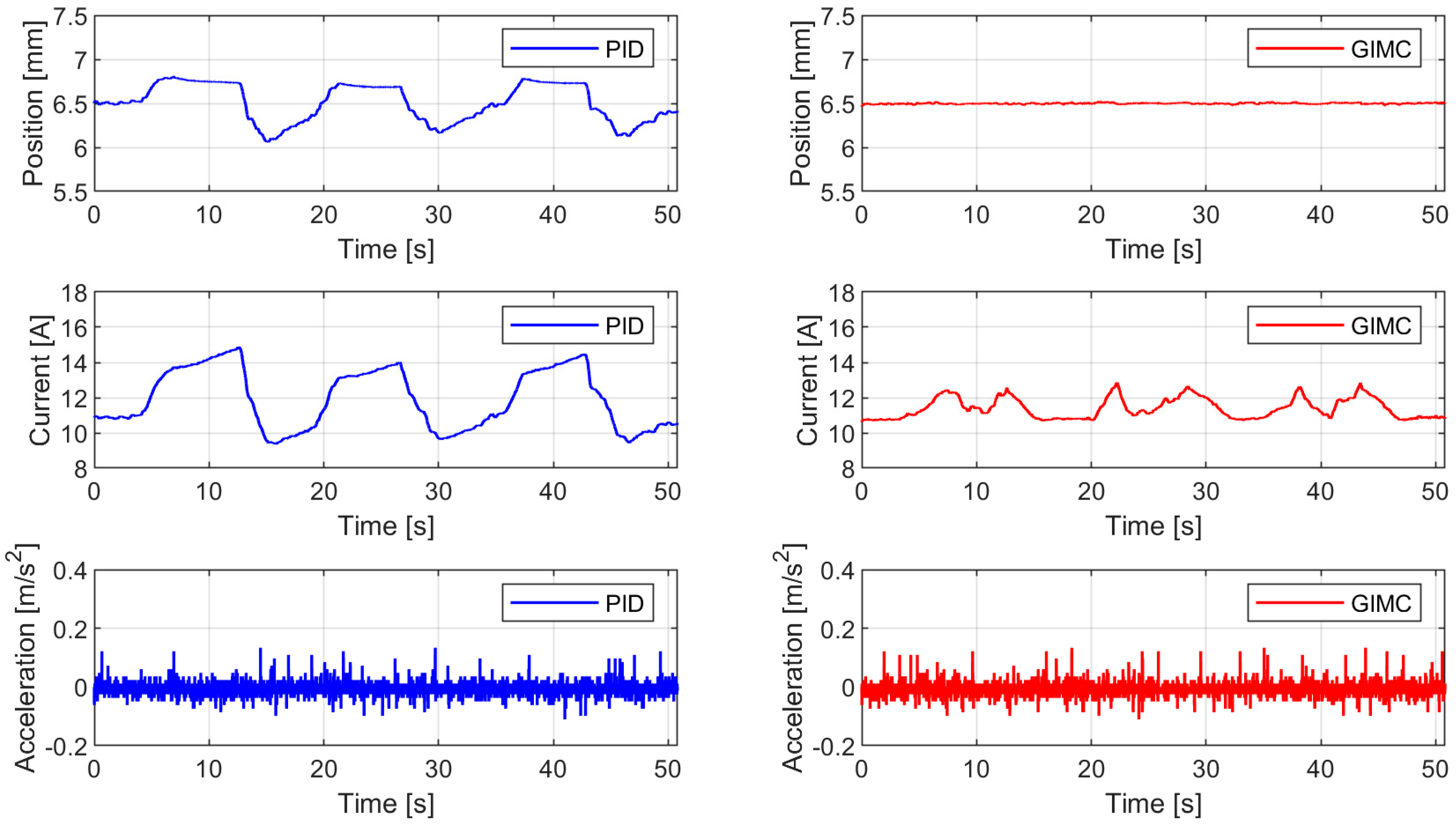
In this section, the experiment is carried out in the small-scale experimental platform shown in Figure 14. The experimental method is shown in Figure 18. When the system is stably suspended at 6.5 mm, slowly apply the lateral force in the horizontal direction with a tension gauge. After the lateral force gradually increases to 98 N (the maximum value of the tension gauge), slowly reduce the lateral force until the system recovers to the nominal suspension state. Repeat the above process three times. During the whole experiment, the gap, current, and acceleration sensors of the suspension system will measure the data of the suspension gap, current, and acceleration. Record and save them through the upper computer. The above process repeats twice, the first time using PID controller, the second time using GIMC controller.

The experimental results are shown in Figure 19. It can be seen that when there is a horizontal misalignment under the action of the lateral force:

(1). If you are using the PID controller (the inner loop is inactive), the suspension gap and current have obvious fluctuations. In general, they will increase as the lateral force increases and will decrease as the lateral force decreases;

(2). If you are using the GIMC controller (the inner loop is active), the suspension gap is almost maintained at 6.5 mm for the whole process and is not affected by external forces and the fluctuation of the suspension current is significantly small;

(3). Under the control of these two algorithms, there are no obvious differences in the suspension acceleration.

Figure 19. The experimental results in the small-scale experimental platform.

Figure 19. The experimental results in the small-scale experimental platform.

5.3. Experiment in the Single-Bogie Experimental Platform

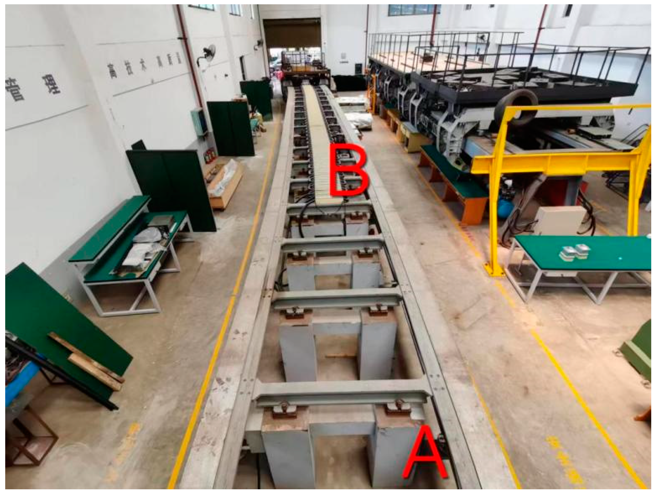
Experimental method: firstly, the single bogie platform should be suspended stably at point A, and the suspension gap is kept at 8 mm, and then it moves slowly from point A to point B; Then floating at point B for a period of time, and then move the single bogie platform from point B to point A slowly. The above process repeats twice. The PID feedback control algorithm is used for the first time and the GIMC algorithm is used for the second time. The curve in experiment scene is shown in Figure 20.

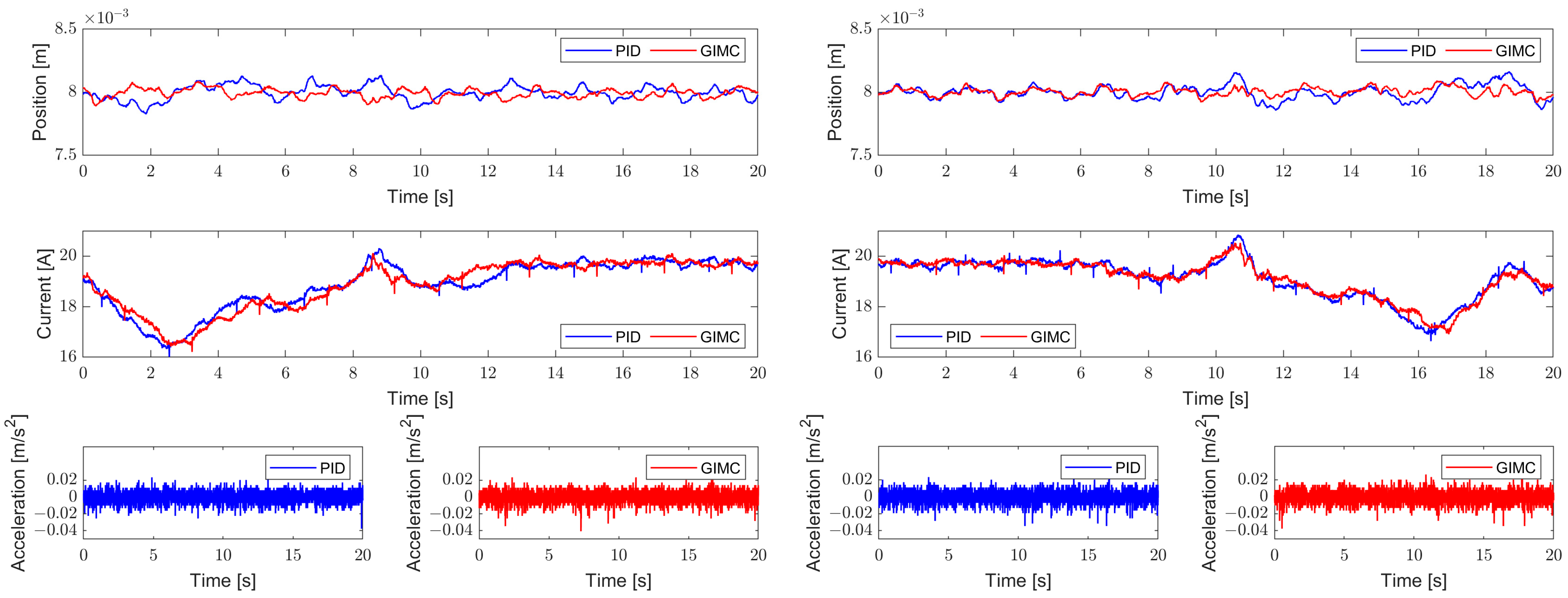
The experimental results are shown in Figure 21. It can be seen that the fluctuation of suspension gap under PID controller is larger than that under GIMC controller, and the variation of suspension current and acceleration are almost the same.

In order to compare the control effects of these two algorithms more carefully, the experimental data are compared quantitatively. The maximum, minimum, average, and variance of experimental data of each group are shown in

Table 3. Quantitative calculation of experimental results about the suspension gap (Unit: mm).

	From Point A to Point B		From Point B to Point A
	PID	GIMC	PID	GIMC
Maximum	8.1360	8.0890	8.1660	8.1070
Minimum	7.8260	7.8890	7.8550	7.9020
Average	7.9975	7.9933	8.0003	8.0044
Variance	3.3891 × 10−3	1.2988 × 10−3	3.4561 × 10−3	1.1607 × 10−3

. It can be seen that under the control of GIMC algorithm, the variance of the suspension gap are smaller both from A to B or from B to A, indicating that the fluctuation range of the suspension gap under the control of GIMC algorithm is smaller.

6. Summary and Prospect

In this article, the horizontal misalignment between the suspension magnet and the rail impacts on suspension system was studied. This problem has attracted the attention of scholars, but the current research mainly focuses on the impact of horizontal misalignment on the guidance system. In fact, many studies have pointed out that the influence of horizontal misalignment on the suspension system cannot be ignored. This article conducts an in-depth analysis on this topic for the first time.

The main innovations and conclusions of this article are:

(1). Considering that the influence of horizontal misalignment on suspension system is mainly reflected in the change of suspension force, this article first analyzes the suspension force in theory and simulation. The results show that the suspension force considering the horizontal misalignment deduced in this article is accurate, and FEA simulation is in good agreement with the results of theoretical derivation.

(2). A suspension system model with uncertainty is established for the first time, which can effectively describe the impact of the horizontal misalignment on the suspension system. This modeling process not only makes the suspension system model more accurate, but also lays a foundation for the controller design.

(3). A controller for the suspension system is designed. This article proves how the controller can effectively suppress the uncertainty caused by the horizontal misalignment theoretically for the first time, so that the suspension system can maintain excellent nominal performance in the case of horizontal misalignment.

(4). The closed-loop system studied in this article is simulated in MATLAB and the experiment is carried out on the small-scale experimental platform and the single-bogie experimental platform. The results show that the proposed control algorithm can effectively suppress the suspension gap and current fluctuation caused by horizontal misalignment.

This research not only solves the problem in theory, but also designs a controller that is suitable for engineering, which has high practicability. In future, we will study other uncertainties of the suspension system and verify whether the GIMC algorithm can still eliminate them.

References

1. Wu, Z.; Jin, J.; Shen, B.; Hao, L.; Guo, Y.; Zhu, J. Fundamental Design and Modelling of the Superconducting Magnet for the High-Speed Maglev: Mechanics, Electromagnetics, and Loss Analysis during Instability. Machines 2022, 10, 113. [Google Scholar] [CrossRef]
2. Zhu, J.; Ge, Q.; Sun, P. Extended state observer-based sensorless control for high-speed maglev application in single-feeding mode and double-feeding mode. IEEE Trans. Transp. Electrif. 2022, 8, 1350–1361. [Google Scholar] [CrossRef]
3. Zhai, D.; Lai, X.; Meng, J.; Liu, G.; Wu, J.; Xiao, S. The hybrid suspension system for middle-to-low-speed maglev trains considering the prevention of firm absorption. IEEE Trans. Transp. Electrif. 2022, 8, 1482–1492. [Google Scholar] [CrossRef]
4. Ma, W.-H.; Luo, S.-H.; Zhang, M.; Sheng, Z.-H. Research review on medium and low speed maglev vehicle. J. Traffic Transp. Eng. 2021, 21, 199–216. (In Chinese) [Google Scholar]
5. Liu, W. Research on system optimization of medium-low speed maglev rail transit tourism characteristics: A case study of qingyuan maglev tourism rail transit. Railw. Stand. Des. 2020, 64, 16–22. (In Chinese) [Google Scholar]
6. Chao, L. Research of Key Technology and Guidance Principle of Low-Speed Maglev Train. Master’s Thesis, Southwest Jiaotong University, Chengdu, China, 2008. (In Chinese). [Google Scholar]
7. Yim, B.H.; Han, H.S.; Lee, J.K.; Kim, S.S. Curving performance simulation of an ems-type maglev vehicle. Veh. Syst. Dyn. 2009, 47, 1287–1304. [Google Scholar] [CrossRef]
8. Han, J.B.; Kim, K.J. Characteristics of vibration in magnetically levitated trains subjected to crosswind. Proc. Inst. Mech. Eng. Part F J. Rail Rapid Transit 2017, 232, 1347–1359. [Google Scholar] [CrossRef]
9. Vesel, V. Robust control methods a systematic survey. J. Electr. Eng. 2013, 64, 59–64. [Google Scholar] [CrossRef] [Green Version]
10. Chang, Y.P. Study on Robust Control for Suspension System in Midium Speed Maglev Train. Ph.D. Thesis, National University of Defense Technology, Changsha, China, 2016. (In Chinese). [Google Scholar]
11. Sun, Y.; Xu, J.; Qiang, H.; Lin, G. Adaptive neural-fuzzy robust position control scheme for maglev train systems with experimental verification. IEEE Trans. Ind. Electron. 2019, 66, 8589–8599. [Google Scholar] [CrossRef]
12. Sun, Y.G.; Xu, J.Q.; Chen, C.; Lin, G.B. Fuzzy H∞ robust control for magnetic levitation system of maglev vehicles based on t-s fuzzy model: Design and experiments. J. Intell. Fuzzy Syst. 2019, 36, 911–922. [Google Scholar] [CrossRef]
13. Sun, Y.G.; Xie, S.; Xu, J.Q.; Lin, G.B. A robust levitation control of maglev vehicles subject to time delay and disturbances: Design and hardware experimentation. Appl. Sci. 2020, 10, 1179. [Google Scholar] [CrossRef] [Green Version]
14. Ni, F.; Mu, S.; Kang, J.; Xu, J. Robust controller design for maglev suspension systems based on improved suspension force model. IEEE Trans. Transp. Electrif. 2021, 7, 1765–1779. [Google Scholar] [CrossRef]
15. Zhou, K.M.; Ren, Z. A new controller architecture for high performance, robust, and fault-tolerant control. IEEE Trans. Autom. Control 2001, 46, 1613–1618. [Google Scholar] [CrossRef] [Green Version]
16. Yubai, K.; Sakuishi, T.; Hirai, J. Compensation of performance degradation caused by fault based on gimc structure: Application to a redundant sensor fault of flexible arm. Electr. Eng. Jpn. 2009, 168, 48–58. [Google Scholar] [CrossRef]
17. Sakuishi, T.; Yubai, K.; Hirai, J. Direct design from input/output data of a fault-tolerant control system based on gimc structure. Electr. Eng. Jpn. 2010, 171, 53–62. [Google Scholar] [CrossRef]
18. Raisemche, A.; Boukhnifer, M.; Larouci, C.; Diallo, D. Experimental gimc fault tolerant control using fixed order H∞ approach for ev induction motor drive. In Proceedings of the 22nd Mediterranean Conference on Control and Automation, Palermo, Italy, 16–19 June 2014. [Google Scholar] [CrossRef]
19. Guo, W.J.; Qiu, A.B.; Li, X. Active fault tolerant control for hvac system based on gimc and feedforward compensation. In Proceedings of the 2019 CAA Symposium on Fault Detection, Supervision and Safety for Technical Processes (SAFEPROCESS), Xiamen, China, 5–7 July 2019. [Google Scholar] [CrossRef]
20. Xue, M.; Xu, G.; Feng, J. Control strategy of automotive electric power steering system based on generalized internal model control. J. Algorithms Comput. Technol. 2020, 14, 1748–3026. [Google Scholar] [CrossRef]
21. Wu, J.; Zhao, Y.Q.; Ji, X. Generalized Internal Model Robust Control for Active Front Steering Intervention. Chin. J. Mech. 2015, 28, 285–293. [Google Scholar] [CrossRef]
22. Xie, W.; Li, G.L. GIMC architecture for linear systems with a single I/O delay. J. Frankl. Inst. 2012, 349, 2151–2162. [Google Scholar] [CrossRef]
23. Brzezina, W.; Langerholc, J. Lift and side forces on rectangular pole pieces in two dimensions. J. Appl. Phys. 1974, 45, 1869–1872. [Google Scholar] [CrossRef]
24. Zhang, N. Parasitic Extraction and Magnetic Analysis for Transformers, Inductors and IGBT Bridge Busbar with Maxwell 2D and Maxwell 3D Simulation. Master’s Thesis, The University of Texas at San Antonio, San Antonio, TX, USA, 2014. (In Chinese). [Google Scholar]
25. Liu, H.; Zhang, Z.; Song, T. ANSYS Maxwell + Workbench 2021 Motor Multi Physical Field Coupling Finite Element Analysis; Chemical Industry Press Co. Ltd.: Beijing, China, 2022; pp. 51–108. (In Chinese) [Google Scholar]
26. Zhao, B.; Zhang, H. Application of Ansoft 12 in Engineering Electromagnetic Field; China Water & Power Press: Beijing, China, 2010; pp. 68–76. (In Chinese) [Google Scholar]
27. Li, Y.G.; Chang, W.S. Cascade control of an ems maglev vehicle’s levitation control system. Agta Autom. Sin. 1999, 25, 247–251. (In Chinese) [Google Scholar]
28. Zhou, K.; Doyle, J.C.; Glover, K. Robust and Optimal Control; Prentice Hall: Englewood Cliffs, NJ, USA, 1995; pp. 117–237. ISBN 9780134565675. [Google Scholar]
Figure 1. The single suspension magnet model. (a) The nominal state; (b) the state existing horizontal misalignment.
Machines 10 00977 g001
Figure 2. The magnetic induction line in suspension gap. (a) The actual state; (b) the approximate state.
Machines 10 00977 g002
Figure 3. Two-dimensional simulation model diagram with horizontal misalignment. (a) y ( t ) = 0 ; (b) y ( t ) = 2 a .
Machines 10 00977 g003
Figure 4. Two-dimensional simulation results with horizontal misalignment (distribution of magnetic induction line). (a) y ( t ) = 0 ; (b) y ( t ) = 2 a .
Machines 10 00977 g004
Figure 5. Attenuation ratio of suspension force with different horizontal misalignments.
Machines 10 00977 g005
Figure 6. The feedback control loop. (a) The feedback control loop composed of K 0 ( s ) and P 0 ( s ) . (b) The feedback control loop is composed of K 0 ( s ) and P ^ 0 ( s ) .
Machines 10 00977 g006
Figure 7. The feedback control loop composed of K ( s ) and P ^ ( s ) .
Machines 10 00977 g007
Figure 8. The equivalent diagram of Figure 7.
Machines 10 00977 g008
Figure 9. Block diagram of the linear fractional transformation.
Machines 10 00977 g009
Figure 10. Block diagram of the small gain theorem.
Machines 10 00977 g010
Figure 11. Block diagram of internal stability analysis.
Machines 10 00977 g011
Figure 13. The improved GIMC control structure for the suspension system.
Machines 10 00977 g013
Figure 14. The small-scale experimental platform of the suspension system.
Machines 10 00977 g014
Figure 15. The single-bogie experimental platform of the suspension system.
Machines 10 00977 g015
Figure 16. The result of simulation 1.
Machines 10 00977 g016
Figure 17. The result of simulation 2.
Machines 10 00977 g017
Figure 18. The experimental method in the small-scale experimental platform. (a) The nominal state; (b) the state existing horizontal misalignment.
Machines 10 00977 g018
Figure 20. Curved rail of physical experiment platform.
Machines 10 00977 g020
Figure 21. The experimental results in the single-bogie experimental platform. (a) From point A to point B; (b) from point B to point A.
Machines 10 00977 g021