Solving the Flexible Job Shop Scheduling Problem Using a Discrete Improved Grey Wolf Optimization Algorithm

Abstract

The flexible job shop scheduling problem (FJSP) is of great importance for realistic manufacturing, and the problem has been proven to be NP-hard (non-deterministic polynomial time) because of its high computational complexity. To optimize makespan and critical machine load of FJSP, a discrete improved grey wolf optimization (DIGWO) algorithm is proposed. Firstly, combined with the random Tent chaotic mapping strategy and heuristic rules, a hybrid initialization strategy is presented to improve the quality of the original population. Secondly, a discrete grey wolf update operator (DGUO) is designed by discretizing the hunting process of grey wolf optimization so that the algorithm can solve FJSP effectively. Finally, an adaptive convergence factor is introduced to improve the global search ability of the algorithm. Thirty-five international benchmark problems as well as twelve large-scale FJSPs are used to test the performance of the proposed DIGWO. Compared with the optimization algorithms proposed in recent literature, DIGWO shows better solution accuracy and convergence performance in FJSPs at different scales.

1. Introduction

Production scheduling is an essential part of modern manufacturing systems, and the efficient scheduling methods can improve industrial production efficiency, increase the economic profitability of enterprises and raise customer satisfaction [1,2,3]. The job shop scheduling problem (JSP) is one of the most complex problems in production scheduling and it has been proven to be NP-hard [4]. The flexible job shop scheduling problem (FJSP) is an extension of JSP. Besides considering operation sequencing, it also needs to assign the appropriate machine to each operation. As the FJSP is more in line with the reality of modern manufacturing enterprises, the problem has been widely studied by many experts and scholars in the past decades [5,6,7]. Furthermore, the problem is increasingly used in different environments, such as crane transportation, battery packaging and printing production [8,9,10].

The first scholars who proposed the FJSP, Brucker and Schlie, used polynomial graph algorithm to solve the problem [11]. With the advance of time, various solution methods were developed for the problem. Up to now, the methods for solving FJSP can be divided into two main categories: exact and approximate algorithms. Exact algorithms—for example, Lagrangian relaxation, branch and bound algorithms and mixed integer linear programming—have the advantage of seeking the optimal solution of the FJSP [12,13,14]. However, they are only effective on small-scale FJSPs, and the computation time required is unaffordable once the size of the problem increases. The second approach has received more attention in recent studies due to its ability to find a better solution in a shorter period of time. Currently, metaheuristic algorithms are a kind of approximation algorithm which have been successfully applied to solve FJSP, such as genetic algorithm (GA), particle swarm algorithm (PSO), ant colony algorithm (ACO), etc.

Initially, research on metaheuristic algorithms for solving FJSPs lies in proposing new neighborhood structures and employing tabu search or simulated annealing algorithms (SA). Brandimarte designed a hierarchical algorithm based on the tabu search for solving FJSP [15]. Based on the characteristics of FJSP, Najid et al. proposed an improved SA for solving the problem [16]. With the objective of minimizing the maximum completion time, Mastrolilli et al. proposed two neighborhood structures (Nopt1, Nopt2) and combined them with TS, and the results validated the effectiveness of the proposed approach [17]. Recent studies have shown that optimizing the objective of the problem by improving the neighborhood structure is an effective method. Zhao suggested a hybrid algorithm that incorporates an improved neighborhood structure. He divided the neighborhood structure into two levels: the first level for moving processes across machines, and the second level for moving processes within the same machine [18]. As the size of FJSP grows, however, the method relying only on improving the neighborhood structure tends to lack diversity in the solution process, which in turn leads to falling into local optimum. Most current researchers solve FJSP by mixing swarm intelligence algorithms with constraint rules of the scheduling problem; the former is used to enhance the diversity of the population, while the latter is employed to exploit the neighborhood of the more optimal solution.

For GA, Li et al. proposed a hybrid algorithm (HA), which combined GA with tabu search (TS) for solving FJSP [19]. The setting of parameters in GA is extremely significant, and a reasonable combination of parameters can better improve the performance of the algorithm. Therefore, Chang et al. proposed a hybrid genetic algorithm (HGA), and the Taguchi method was used to optimize the parameters of the GA [20]. Similarly, Chen et al. suggested a self-learning genetic algorithm (SLGA) to solve the FJSP and dynamically adjusted its key parameters based on reinforcement learning (RL) [21]. Wu et al. designed an adaptive population nondominated ranking genetic algorithm III, which combines a dual control strategy with GA to solve FJSP considering energy consumption [22].

For ACO, Wu et al. proposed a hybrid ant colony algorithm based on a three-dimensional separation graph model for a multi-objective FJSP in which the optimization objectives are makespan, production duration, average idle time and production cost [23]. Wang et al. presented an improved ant colony algorithm (IACO) to optimize the makespan of FJSP, which was tested by a real production example and two sets of well-known benchmark test examples to verify the effectiveness [24]. To solve the FJSP in a dynamic environment, Zhang et al. combined Multi-Agent System (MAS) negotiation and ACO, and introduced the features of ACO into the negotiation mechanism to improve the performance of scheduling [25]. Tian et al. introduced a PN-ACO-based metaheuristic algorithm for solving energy-efficient FJSP [26].

For PSO, Ding et al. suggested a modified PSO for solving FJSP, and obtained useful solutions by improved encoding schemes, communication mechanisms of particles and modification rules for operating candidate machines [27]. Fattahi et al. proposed a hybrid particle swarm optimization and parallel variable neighborhood search (HPSOPVNS) algorithm for solving a flexible job shop scheduling problem with assembly operations [28]. In real industrial environments, unplanned and unforeseen events have existed. Considering the FJSP under machine failure, Nouiri et al. proposed a two-stage particle swarm optimization algorithm (2S-PSO), and the computational results showed that the algorithm has better robustness and stability compared with literature methods [29].

There has been an increasing number of studies on solving the FJSP using other metaheuristic algorithms in recent years. Gao et al. proposed a discrete harmonic search (DHS) algorithm based on a weighting approach to solve the bi-objective FJSP, and the effectiveness of the method was demonstrated by using well-known benchmark examples [30]. Feng et al. suggested a dynamic opposite learning assisted grasshopper optimization algorithm (DOLGOA). The dynamic opposite learning (DOL) strategy is used to improve the utilization capability of the algorithm [31]. Li et al. introduced a diversified operator imperialist competitive algorithm (DOICA), which requires minimum makespan, total delay, total work and total energy consumption [32]. Yuan et al. proposed a hybrid differential evolution algorithm (HDE) and introduced two neighborhood structures to improve the search performance [33]. Li et al. designed an improved artificial bee colony algorithm (IABC) to solve the multi-objective low-carbon job shop scheduling problem with variable processing speed constraints [34].

Table 1. Literature review of various popular algorithms for solving FJSP.

Method		Representative Algorithms	Advantages and Disadvantages
Exact algorithm	Enumerative methods	Lagrangian relaxation, branch and bound method and mixed integer linear programming	The optimal solution can be obtained, but the execution time is unbearable
Approximate algorithm	Local search algorithm	Tabu search, variable neighborhood search and simulated annealing	Excellent local search capability, but poor diversity
	Swarm intelligence algorithm	Particle swarm, ant colony and artificial bee colony algorithms	Suitable diversity, but easily falls into local optimum

shows a literature review of various common algorithms for solving FJSP.

The grey wolf optimization (GWO) algorithm is a population-based evolutionary metaheuristic algorithm proposed by Mirjalili in 2014, which was originally presented for solving continuous function optimization problems [35]. In GWO, the hierarchical mechanism and hunting behaviors of the grey wolf population in nature are simulated. Compared with other metaheuristic algorithms, the GWO algorithm has the advantages of simple structure, few control parameters and the ability to achieve a balance between local and global search. It has been successfully applied to several fields in recent years, such as path planning, SVM model, image processing, power scheduling, signal processing, etc. [36,37,38,39,40]. However, the algorithm is rarely used on FJSP. As the algorithm is continuous and FJSP is a discrete problem, it is important to consider how to match the algorithm with the problem.

At the moment, there are two mainstream solution methods. The first method adopts a transformation mechanism to interconvert continuous individual position vectors with discrete scheduling solutions, which has the advantage of being simple to implement and preserving the updated iterative formulation of the algorithm. Luan et al. suggested an improved whale optimization algorithm for solving FJSP, in which ROV rules are used to transform the operation sequence [41]. For FJSP, Yuan et al. proposed a hybrid harmony search (HHS) algorithm and developed a transformation technique to convert a continuous harmony vector into a discrete two-vector code for FJSP [42]. Luo et al. designed the multi-objective flexible job shop scheduling problem (MOFJSP) with variable processing speed, for which the chromosome encoding is represented by a three-vector representation corresponding to three subproblems: machine assignment, speed assignment and operation sequence. The mapping approach and the genetic operator are used to enable the algorithm to update in the discrete domain [43]. Liu et al. proposed the multi-objective hybrid salp group algorithm (MHSSA) mixed with Lévy flight, random probability crossover operator and variational operator [44]. Nevertheless, the transformation method has certain limitations—some excellent solutions will be missed in the process of conversion, and a lot of computation time will be wasted.

In the second approach, the discrete update operator is designed to achieve the correspondence between the algorithm and the problem. For the multi-objective flexible job shop scheduling problem, a hybrid discrete firefly algorithm (HDFA) was proposed by Karthikeyan et al. The search accuracy and information sharing ability of the algorithm are improved by discretization [45]. Gu et al. suggested a discrete particle swarm optimization (DPSO) algorithm and designed the discrete update process of the algorithm by using crossover and variational operators [46]. Gao et al. studied a flexible job shop rescheduling problem for new job insertion and discretized the update mechanism of the Jaya algorithm, and the results of extensive experiments showed that the DJaya algorithm is an effective method for solving the problem [47]. Xiao et al. suggested a hybrid algorithm combining the chemical reaction algorithm and TS, and designed four basic operations to ensure the diversity of populations [48]. Jiang et al. presented a discrete cat swarm optimization algorithm in order to solve a low-carbon flexible job shop scheduling problem with the objective of minimizing the sum of energy cost and delay cost, and designed discrete forms for the finding and tracking modes in the algorithm to fit the problem [49]. Lu et al. redesigned the propagation, refraction and breaking mechanisms in the water wave optimization algorithm based on the characteristics of FJSP in order to adapt the algorithm to the scheduling problem under consideration [50]. Although this method discards the update formula, the idea of the algorithm is retained. Thus, it is essential to design a more reasonable discrete update operator. At present, there is already a method for the discretization of the GWO operator for solving FJSP, but the method simply retains the process of the head wolf guiding the ordinary wolf hunting in the wolf pack, and does not facilitate more excavation of GWO [51].

Table 2. Literature review of conversion methods.

References	Objective Type	Method	Algorithm	Characteristic
[41]	Makespan	Conversion	IWOA	ROV conversion rule
[42]	Makespan	Conversion	HHS	LPV mapping rule
[43]	Makespan and total energy consumption	Conversion	GWO	Ascending mapping
[44]	Makespan, total worker costs and total influence of the green production	Conversion	HSSA	Ascending mapping
[45]	Makespan, critical machine load and total machine load	Discretization	HDFA	Hamming Distance
[46]	Makespan, critical machine load and total machine load	Discretization	DPSO	Crossover and mutation update operators
[47]	Makepsan, total flow time, critical machine load and total machine load	Discretization	DJaya	DJaya update operator
[48]	Makepsan	Discretization	CROTS	Discrete collision and decomposition reactions
[49]	Energy consumption and cost	Discretization	CSO	Discrete seeking and tracing modes
[50]	Energy consumption and makespan	Discretization	DWWO	Discrete propagation, refraction and breaking behavior

contains a literature review on mapping mechanisms and discrete operators in FJSP.

In view of this, a discrete improved grey wolf optimization algorithm (DIGWO) is proposed in this paper for solving FJSP with the objectives of minimizing makespan and minimizing critical machine load. The algorithm has the following innovations. Firstly, a discrete grey wolf update operator is proposed in order to make GWO applicable for solving FJSP. Secondly, an initialization method incorporating the chaotic mapping strategy and heuristic rule is designed to obtain high high-quality and diverse initial populations. Then, an adaptive convergence factor is employed to make the algorithm better balanced in exploitation and exploration. Finally, the effectiveness as well as the superiority of the proposed algorithm are verified using international benchmark cases.

The contributions of this paper are in the following five aspects.

• A hybrid initialization method which combines heuristic rules and random Tent chaotic mapping strategy is proposed for generating original populations with high quality and without loss of diversity.
• For the characteristics of FJSP, a discrete grey wolf update operator is designed to improve the search performance of the algorithm while ensuring that the algorithm can solve the problem.
• An adaptive convergence factor is proposed to improve the exploration and exploitation capability of the algorithm.
• The improved algorithm is applied to solve the benchmark test problems in the existing literature, and the results show that DIGWO is competitive compared to other algorithms.
• The performance of DIGWO was executed on 47 FJSP instances of different sizes, and the experimental results show the effectiveness of DIGWO in solving this problem under this condition.

The sections of this paper are organized as follows. Section 1 is an introduction, and it gives the background of the topic as well as the motivation for the research. In Section 2, the mathematical models of the multi-objective FJSP and the original GWO are given. The specific steps of the improvement strategy are described in detail in Section 3. In Section 4, the performance of the proposed DIGWO is tested on continuous-type benchmark functions. The effectiveness of DIGWO is verified using the international standard FJSP in Section 5. Finally, the work is summarized and directions for future research are proposed.

2. Mathematical Models of FJSP

2.1. Problem Description

FJSP is an idealized combinatorial optimization problem induced from actual shop production. Initially, FJSP was derived from JSP. In JSP, the items to be produced are uniformly defined as jobs which have one or more steps. The steps are defined as operations, and the equipment used to process the job is uniformly defined as machines in the process. JSP has the constraint of job sequencing, i.e., each job is processed on its corresponding machine according to a certain processing flow until all jobs are processed. Therefore, FJSP can be considered as an extended version of JSP due to the fact that it eliminates some of the machine constraints and because the number of machines that can be selected for each operation is not limited to only one.

There is one more significant classification that needs to be clarified before solving for FJSP. That is, it can be classified according to the number of machines that can be selected for the operation: total FJSP (T-FJSP) and partial FJSP (P-FJSP). As can be seen from the above, FJSP breaks through the singularity of the number of machines that can be selected for an operation, and if all operations can be processed by any machine, this case is defined as T-FJSP. If there are operations that cannot be processed on certain machines, then this situation can be classified as P-FJSP. Compared to T-FJSP, P-FJSP is more universal, so this study focuses on P-FJSP [52]. An example of a 3 × 3 scale P-FJSP is shown in

Table 3. An instance of 3 × 3 P-FJSP.

Job (n)	Operation (g)	Machines (m)
		M1	M2	M3
1	1	3	5	7
	2	6	-	3
2	1	-	6	4
	2	5	4	5
	3	2	-	-
3	1	5	7	-
	2	-	3	-
	3	4	6	5

, where the first two columns indicate the job number and operation number, and the rest of the data represent the machines that can be selected for operational processing and their corresponding processing times. It can be clearly seen that operation 1 of job 1 is allowed to be processed on all three machines, while operation 3 of job 2 and operation 1 of job 3 are allowed to be processed on only a part of the machines.

A P-FJSP of size $n\times m$ is described as follows: there are $n$ mutually independent jobs $J=\left\{J_1,J_2,\dots J_n\right\}$ assigned to $m$ machines $M=\left\{M_1,M_2,\dots M_m\right\}$ for processing. Each job contains several operations, for example, the $i$th job $J_i$ in the job set contains $g$ operations $\left\{O_{i,1},O_{i,2},\dots ,O_{i,g}\right\}$. It is important to note that the processing time for operating $O_{i,j}$ varies with the machine selected due to the different processing capabilities of the machines. The task of scheduling in this paper is to assign jobs to corresponding machines and to adjust the processing order, subject to several constraints, and to optimize the makespan and the critical machine load; the mathematical model of FJSP can be found in the literature [53]. The constraints satisfied by FJSP are as follows.

• All machines can be started at time 0.
• Different jobs have the same processing priority, and different operations within the same job have different priorities.
• Only one operation can be processed by a machine at the same time.
• Once the machine is running, the process is not interrupted.
• Operations are performed in a preset processing order and one operation can only be processed by the machine once.
• Machine failures do not occur.
• The time spent on the transfer and setup of the machine is not taken into account.

2.2. Model of FJSP

A two-objective FJSP is considered, and its main purpose is to assign each job to the corresponding machine according to the processing constraints. A scheduling table that ensures minimum makespan and minimum critical machine load is finally obtained. The objective function can be represented by Equations (1) and (2) with some constraints. For better understanding, the notations and variables mentioned in the problem model below are given in

Table 4. Notation definitions and abbreviations in the article.

Notations and Abbreviations	Description
$i$	$\mathrm{Index}\mathrm{of}\mathrm{jobs},i=\left\{1,2,\dots ,n\right\}$
$j$	$\mathrm{Index}\mathrm{for}\mathrm{operation}\mathrm{of}\mathrm{job},j=\left\{1,2,\dots ,g\right\}$
$k$	$\mathrm{Index}\mathrm{of}\mathrm{machines},k=\left\{1,2,\dots ,m\right\}$
$n$	Total number of jobs
$m$	Total number of machines
$g$	The number of operations contained in the current job
$J$	The set of all jobs
$M$	The set of all machines
$M_k$	The $k$th machine in $M$
$J_i$	The $i$th job in $J$
$O_{i,j}$	The operation $j$ of job $i$
$s_{i,j,k}$	The start time of operation $j$ of job $i$ on machine $k$
$t_{i,j,k}$	The processing time of operation $j$ of job $i$ on machine $k$
$e_{i,j,k}$	The end time of operation $j$ of job $i$ on machine $k$
$X_{i,j,k}$	Decision variable: if operation $j$ of job $i$ is processed on machine $k$, then 1; otherwise, 0
$C_{max}$	Makespan
$W{L}_k$	The workload on machine $k$
$HI$	Hybrid initialization
$DGUO$	Discrete grey wolf update operator
$MS$	Machine sequence
$OS$	Operation sequence
$ub$	The upper boundary of the search space
$lb$	The lower boundary of the search space
IPOX	Improved priority operation crossover
MPX	Multi-point crossover

, along with the abbreviations commonly used in the article.

Objective:

$$min{F}_1=\begin{array}{cc}min\left(C_{max}\right)=min\{max{\displaystyle \sum _{i=1}^n}{\displaystyle \sum _{j=1}^g}\left(s_{i,j,k}+t_{i,j,k}\right)\},\hfill & \hfill 1\le i\le n\hfill \end{array}$$

(1)

$$min{F}_2=mmin\left(W{L}_k\right)=\begin{array}{cc}min\left(max\left({\displaystyle \sum _{i=1}^n}{\displaystyle \sum _{j=1}^g}{t}_{i,j,k}\ast X_{i,j,k}\right)\right),\hfill & \hfill 1\le k\le m\hfill \end{array}$$

(2)

$C_{max}$ denotes the largest makespan of all jobs, $s_{i,j,k}$ represents the start time of operation $j$ of job $i$ on machine $k$,$e_{i,j,k}$ is the end time of operation $j$ of job $i$ on machine $k$ and $t_{i,j,k}$ denotes the processing time of operation $j$ of job $i$ on machine $k$. $W{L}_k$ is the workload on machine $k$.

Subject to:

$$t_{i,j,k}>0,i=1,2,\dots ,n;j=1,2,\dots ,g;k=1,2,\dots ,m.$$

(3)

$$s_{i,j,k}+t_{i,j,k}\le e_{i,j,k}$$

(4)

$${\displaystyle \sum }_{k=1}^m{X}_{i,j,k}=1$$

(5)

$${\displaystyle \sum }_{i=1}^n{\displaystyle \sum }_{j=1}^g{X}_{i,j,k}=1$$

(6)

$$X_{i,j,k}=\left\{\begin{array}{cc}1\hfill & \hfill when\mathrm{operation}j\mathrm{of}\mathrm{job}iisassignedtomachinek\hfill \\ 0\hfill & \hfill otherwise\hfill \end{array}\right.$$

(7)

The constraint in Equation (3) indicates that the processing time of each operation is greater than 0. The constraints in Equation (4) ensure that the same job contains operations with different levels of priority constraints between them. The constraint in Equation (5) indicates that each operation is only assigned to one machine, and the constraint in Equation (6) ensures that each machine can only process one operation at any time. Constraint (7) is a decision variable that indicates whether the operation $O_{i,j}$ is assigned to machine $M_k$.

2.3. Basic GWO Algorithm

GWO is a novel metaheuristic algorithm proposed by Mirgalili et al. in 2014, inspired by the habits of grey wolf packs, and the algorithm works by mimicking the hierarchical stratification and prey attack behavior within the wolf pack [35]. Grey wolves live in packs, with an average of 5 to 12 wolves per pack. The characteristics of GWO are described below. In the hierarchical stratification mechanism, all individuals in the population can be divided into four classes according to their status. As shown in Figure 1, the alpha (α), beta (β), delta (δ) and omega (ω) wolves are in the order from top to bottom. The α is the first rank, which is responsible for making decisions on group actions in the population. The second level is β. This level is responsible for assisting α wolves, and when α wolves die or become old, β wolves will be promoted to the status of α wolves. The δ wolf plays the role of the trainer of the α wolf in the pack, and it is responsible for reinforcing the orders of the α wolf to the bottom level wolves. The last level of the wolf pack is the ω wolf, and they need to follow the orders of the first three levels of wolves to complete their required tasks.

The update mechanism of GWO is divided into the following parts: surrounding prey, hunting, attacking prey and searching for prey. The grey wolf pack is guided forward by the leader wolf, and because the individual position of the prey cannot be identified in the abstract model, the three leader wolves are approximated as the possible positions of the prey.

2.3.1. Encircling Prey

The process of encircling the prey by the grey wolf can be represented by a mathematical model shown in Formulas (8) and (9).

$$\overrightarrow{D}=|\overrightarrow{C}·{\overrightarrow{X}}_p\left(t\right)-\overrightarrow{X}\left(t\right)|$$

(8)

$$\overrightarrow{X}\left(t+1\right)={\overrightarrow{X}}_p-\overrightarrow{A}·\overrightarrow{D}$$

(9)

where $\overrightarrow{X}\left(t+1\right)$ represents the position vector of the next generation of the grey wolf, ${\overrightarrow{X}}_p\left(t\right)$ denotes the position vector of the prey, $\overrightarrow{X}\left(t\right)$ indicates the current position vector of the grey wolf and $\overrightarrow{D}$ is the absolute distance between the grey wolf and the prey. The coefficient vectors A and C are calculated as follows:

$$\overrightarrow{A}=2\overrightarrow{a}\cdot {\overrightarrow{r}}_1-\overrightarrow{a}$$

(10)

$$\overrightarrow{C}=2\cdot {\overrightarrow{r}}_2$$

(11)

where $\overrightarrow{a}$ has self-adaptive property and decreases linearly from 2 to 0 with increasing iterations, ${\overrightarrow{r}}_1$ and ${\overrightarrow{r}}_2$ are random vectors in the range [0, 1].

2.3.2. Hunting

In the process of hunting, the position of the prey is known to the wolf pack; however, the position of the optimal solution cannot be determined in the abstract search process. Therefore, the position of the individual is updated according to the three best solutions so far: alpha, beta and delta. This process can be represented by a mathematical model shown in Equations (12)–(14).

$$X\left(t+1\right)=\frac{X_1\left(t\right)+X_2\left(t\right)+X_3\left(t\right)}{3}$$

(12)

$${\overrightarrow{X}}_1={\overrightarrow{X}}_{\alpha }-{\overrightarrow{A}}_1·({\overrightarrow{D}}_{\alpha }),{\overrightarrow{X}}_2={\overrightarrow{X}}_{\beta }-{\overrightarrow{A}}_2·({\overrightarrow{D}}_{\beta }),{\overrightarrow{X}}_3={\overrightarrow{X}}_{\delta }-{\overrightarrow{A}}_3·({\overrightarrow{D}}_{\delta })$$

(13)

$${\overrightarrow{D}}_{\alpha }=|\overrightarrow{C_1}·{\overrightarrow{X}}_{\alpha }-\overrightarrow{X}|,{\overrightarrow{D}}_{\beta }=|\overrightarrow{C_2}·{\overrightarrow{X}}_{\beta }-\overrightarrow{X}|,{\overrightarrow{D}}_{\delta }=|\overrightarrow{C_3}·{\overrightarrow{X}}_{\delta }-\overrightarrow{X}|$$

(14)

where $X_1\left(t\right)$, $X_2\left(t\right)$ and $X_3\left(t\right)$ denote the movement steps of individual grey wolves in three directions. ${\overrightarrow{X}}_{\alpha }$, ${\overrightarrow{X}}_{\beta }$ and ${\overrightarrow{X}}_{\delta }$ represent the position vectors of the three head wolves. ${\overrightarrow{A}}_1$, ${\overrightarrow{A}}_2$ and ${\overrightarrow{A}}_3$ denote the coefficient vectors. ${\overrightarrow{D}}_{\alpha }$, ${\overrightarrow{D}}_{\beta }$ and ${\overrightarrow{D}}_{\delta }$ show the distance of the current grey wolf individual to the alpha wolf, beta wolf and delta wolf, respectively.

2.3.3. Attacking Prey and Search for Prey

The behaviors of attacking prey and searching for prey in GWO correspond to the exploitation and exploration of the algorithm, and these two processes are determined by the control parameters A and C. It is known by the above description that A is a random value in the interval $\left[-2a,2a\right]$. When |A|<1, the grey wolf will attack in the direction of the prey, and on the contrary, the grey wolf will be forced to move away from the prey. This means that the unknown space will be explored as much as possible in the early stages of the algorithm iteration. In the middle and late stages of the iteration, |A| will be greater than 1 with high probability, which is beneficial to make the population move quickly to a more desirable area. Compared to vector A, it is important to note that the C vector is characterized by a random value rather than a linear descent throughout the algorithm update process. Therefore, the stochastic nature of the C vector means that its emphasis is on exploration ability, which is more significant to help the algorithm in the later iterations.

3. Proposed Discrete Improved Grey Wolf Optimization Algorithm

3.1. The Framework of the Proposed DIGWO

In this paper, a discrete improved grey wolf optimization algorithm (DIGWO) is proposed. In order to apply GWO to solve FJSP as well as to enhance the search capability of the algorithm, DIGWO contains three improved strategies, namely hybrid initialization (HI), discrete grey wolf update operator (DGUO) and adaptive convergence factor. The process of discretization follows the basic principles of GWO, in which the update operator of the evolutionary algorithm is used and the key parameters in GWO are retained. The flowchart of DIGWO is shown in Figure 2. The steps of the algorithm are as follows.

Step 1: Input the parameters of the algorithm, the information of the FJSP case and the termination conditions, etc.

Step 2: Initialize the population and calculate the fitness of all individuals (c.f. Section 3.3).

Step 3: Determine whether the termination condition is reached—if yes, go to step 9; otherwise, go to step 4.

Step 4: Three optimal individuals in the population are labeled according to the size of the fitness, namely Xalpha, Xbeta and Xdelta.

Step 5: Update the control parameters $a$ and $A$ (c.f. Section 3.4).

Step 6: Update all individuals in the population using the DGUO, with different update mechanisms for common and alpha wolves (c.f. Section 3.5.1 and Section 3.5.2).

Step 7: The offspring grey wolf individuals were selected and preserved according to the acceptance probability $p_{accept}$ (c.f. Section 3.5.3).

Step 8: Determine if the termination condition is met—if yes, go to step 9; otherwise, return to step 4.

Step 9: Output the optimal solution and its coding sequence.

In order to elaborate the proposed DIGWO more carefully, the key strategies of the algorithm as well as the parameters are mainly discussed below, and the algorithm is thoroughly analyzed in the subsequent sections. In the proposed DIGWO, two key parameters are defined: the control parameter $\lambda$ in the adaptive convergence factor $A$ and the distance acceptance probability $p_{accept}$. These two key parameters are described in detail in Section 3.4 and Section 3.5.3.

In the initialization phase, the modified Tent chaotic mapping is used to generate the operation sequences and the heuristic rules are used to generate the machine sequences. The specific initialization steps can be found in Section 3.3. Next, in the update phase of the algorithm, the improved convergence factor is used to optimize the balance between global search and local search for DIGWO. The specific improved formula can be found in Section 3.4. Before introducing DGUO, it is important to highlight that the encoding type of DIGWO is discrete during solving FJSP. Therefore, the update formula of the original GWO is no longer used, and the discrete update operator is designed according to the characteristics of the FJSP. The following steps are followed in one update of the algorithm. The population was divided into two parts, the leader wolves and the ordinary wolves. Firstly, the ordinary wolves of the population are updated, and the mode of updating is determined by the value of the adaptive convergence factor $A$. If $\left|A\right|<1$, then the appropriate leader wolf is selected by roulette and updated in the discrete domain. On the contrary, an individual in the population of ordinary wolves is selected for updating. Secondly, the leader wolves are updated. For the operation sequence and machine sequence of the leader wolves, the neighborhood adjustment based on the critical path is adopted. Finally, the traditional elite strategy and the reception criterion based on distance proposed in this paper are combined to generate new populations, and the individuals of leader wolves and ordinary wolves are merged for the next iteration of updating. The detailed description of DGUO can be found in Section 3.5.

3.2. Solution Representation

The solution of the proposed algorithm contains two vectors: the machine selection vector and the operation sequence vector. In order to represent these two subproblems more rationally, an integer coding approach is adopted in this paper. Next, the 3 × 3 FJSP example in Table 3 is used to explain the encoding and decoding methods.

The machine selection (MS) vector is made up of an array of integers. The encoding of the machine sequence corresponds to the order of the job numbers from the smallest to the largest, as shown in Figure 3. The machine sequence can be expressed as $\mathrm{MS}=\left\{2,3,3,3,1,1,2,1\right\}$. It should be noted that each element in the MS sequence represents the machine number; for example, the fourth element of the MS indicates that machine $M_3$ is selected by operation 1 of job 2.

The operation sequence (OS) vector consists of an array of integers, representing the job information and operation processing order in FJSP. As shown in Figure 3, the operation sequence can be expressed as $\mathrm{OS}=\left\{3,2,1,1,3,1,2,3\right\}$. It should be noted that the elements in the OS vector are represented by job numbers. In the order starting at the left, if the element of the OS at the $n$th position is $i$ and it appears $j$ times in the current sequence, the element correspond to the information about operation $j$ of job $i$ and is $O_{i,j}$. Therefore, it can be seen from the OS vector in Figure 3 that the decoding order is $O_{3,1}\to O_{2,1}\to O_{1,1}\to O_{1,2}\to O_{3,2}\to O_{1,3}\to O_{2,2}\to O_{3,2}$. 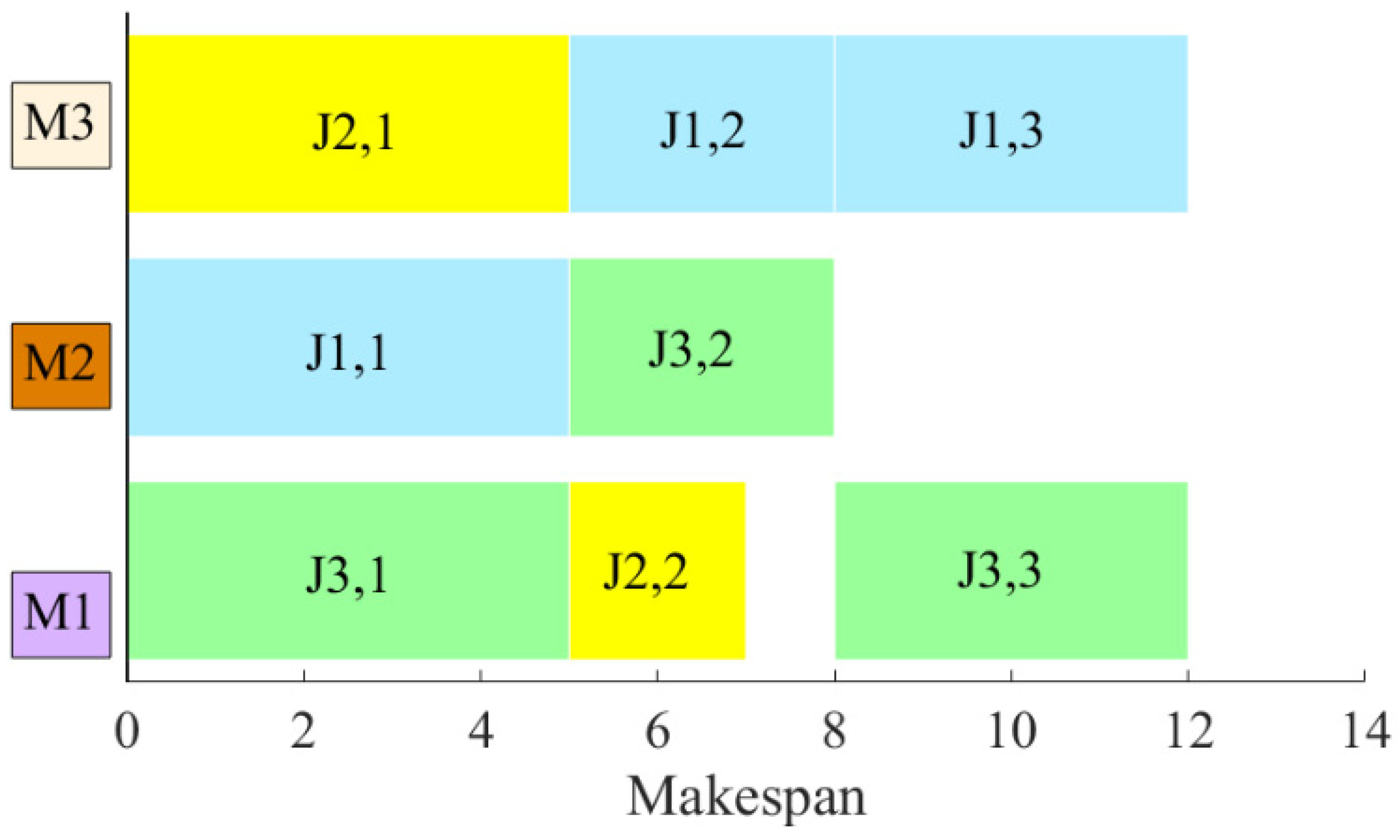The decoding process is as follows. First, all operations are assigned to the corresponding machines based on the MS vector. Meanwhile, the processing order of all operations on each machine is determined by the OS vector. Then, the earliest start time of the current operation is determined according to the constraint rules of FJSP. Finally, a reasonable scheduling scheme is obtained by arranging all operations to their corresponding positions. 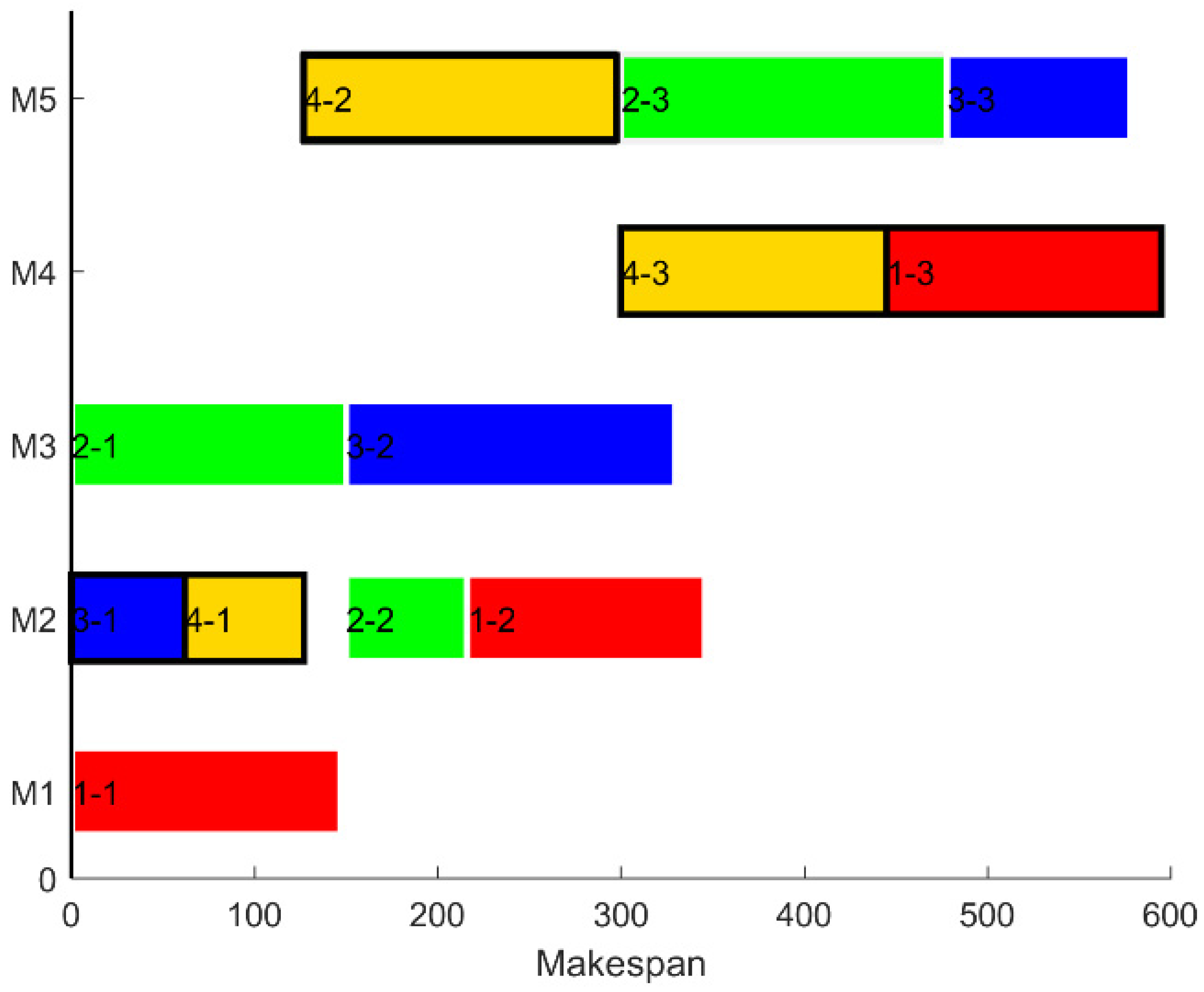Figure 4 shows the Gantt chart of a 3 × 3 FJSP instance.

3.3. Population Initialization

For swarm intelligence algorithms, the quality of the original population can be improved by effective initialization methods, and it is able to give a positive impact during the subsequent iterations. Currently, most of the initialization methods in studies about FJSP use random methods to generate populations. Nevertheless, it is difficult to guarantee the quality of the generated initial populations by only using random methods. Consequently, it is important to design effective strategies for the initialization phase to improve the search performance of the algorithm.

Tent chaotic sequences, with their favorable randomness, ergodicity and regularity, are often used to combine with metaheuristic algorithms to improve population diversity and enable the algorithm’s global search capability [54]. In this paper, a modified Tent chaotic sequence is introduced, and its expression is shown in Formula (15). The variables obtained by Tent chaotic mapping in the search space are shown in Equation (16).

$$y_{j+1}^i=\left\{\begin{array}{cc}2y_j^i+rand\left(0,1\right)\times \frac{1}{N}& y_j^i\in \left[0,\frac{1}{2}\right]\\ 2\left(1-y_j^i\right)+rand\left(0,1\right)\times \frac{1}{N}& y_j^i\in \left(\frac{1}{2},1\right]\end{array}\right.$$

(15)

$$x_j^i=l{b}^i+\left(u{b}^i-l{b}^i\right)y_j^i$$

(16)

where $rand\left(0,1\right)$ is the random number within the interval [0, 1], $i$ is the individual number, $j$ is the number of the chaotic variable, $N$ is the total number of individuals within the population and $ub$ and $lb$ are the upper and lower bounds of the current variable in the search space, respectively.

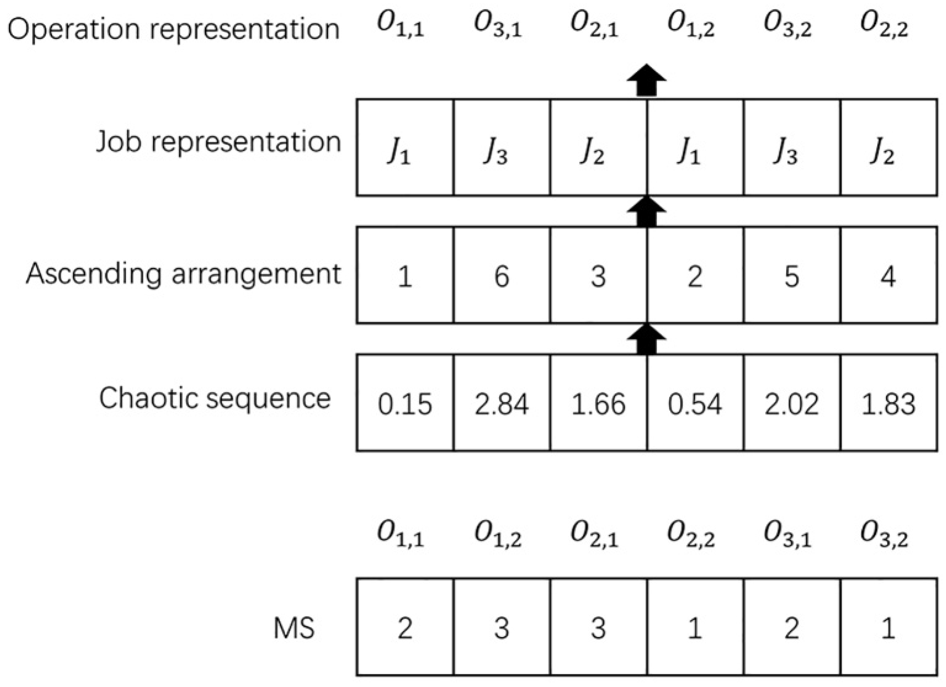
As shown in Figure 5, the machines are selected for the current operation in order from left to right according to the code, and the MS is finally obtained. A string of position index codes is obtained by arranging the obtained chaotic sequence in ascending order, and then transformed into an operation sequence according to the distribution of jobs and their operations. In Figure 5, the chaotic sequence {0.15, 2.84, 1.66, 0.54, 2.02, 1.83} is transformed into the operation codes {$O_{1,1},O_{3,1},O_{2,1},O_{1,2},O_{3,2},O_{2,2}\}$.

Three heuristic strategies are introduced in the initialization phase of the machine sequence to improve the quality of the initial population. Combined with the chaotic mapping strategy, these three strategies are described as follows.

Random initialization: This is the earliest initialization method, and the reason for adopting this strategy is that it guarantees a high diversity of the initial populations generated. (1) Generate a sequence of operations by chaotic mapping. (2) Randomly select a machine from its corresponding set of select machines for the current operation, in left-to-right order. (3) Repeat step 2 until a complete vector of machines is generated.

Local processing time minimization rule: The purpose of this rule is to select a machine with the minimum processing time for each operation, thus reducing the corresponding processing time [55]. (1) Generate a sequence of operations by chaotic mapping. (2) Select a machine with the minimum processing time for the current operation from its corresponding set of available machines, in left-to-right order. (3) Repeat step 2 until a complete vector of machines is generated.

Minimum completion time: The purpose of this rule is to optimize the maximum completion time and prevent over-selection of the machine with the smallest processing time, which could lead to a machine with high performance but too many operations scheduled to be processed, while a machine with low performance is left idle [56]. (1) Generate a sequence of operations by chaotic mapping. (2) In left-to-right order, if the selectable machines for the current operation are greater than or equal to two, determine the machine with the smallest completion time based on the earliest start time and processing time. (3) Repeat step 2 until a complete vector of machines is generated.

Each of the three strategies mentioned above has been proven effective in the literature, so a hybrid initialization approach (HI) is proposed by combining the advantages of the three strategies. The strategy is described in Algorithm 1.

Algorithm 1. Hybrid initialization (HI) strategy
Input: Total number of individuals $n$
Output: Initial population
1.	for $i$ = 1:$n$ do
2.	The initial population is generated using a random initialization rule, size [$n/3$]
3.	The initial population is generated employing the local minimum processing time rule, size [$n/3$]
4.	The initial population is generated applying the minimum completion time rule, size [$n/3$]
5.	Combine the initial populations generated by the above three rules, denoted as $P$
6.	if size of $P=n$ then
7.	break
8.	else
9.	Generate the rest with a random initialization strategy
10.	end if
11.	end for

3.4. Nonlinear Convergence Factor

Needless to say, the primary consideration for metaheuristics is how to better balance the exploration and exploitation capabilities of the algorithm. This is no exception in GWO. The parameter A, in the traditional GWO, plays the role of regulating the global and local search capability of the algorithm. Throughout the search process of the algorithm, |A| < 1, the ordinary wolf will move in the direction of the head wolf individual in the population, which reflects the local search of the algorithm. On the contrary, the grey wolf individuals will move away from the head wolf, which corresponds to the global search ability of the algorithm. The change in parameter A is determined by the linearly decreasing parameter $a$. Nevertheless, since FJSP itself is a combinatorial optimization problem with high complexity, it is difficult to accurately adapt to the complex nonlinear search process if only the traditional parameter $a$ of GWO is used to control the update of the algorithm.

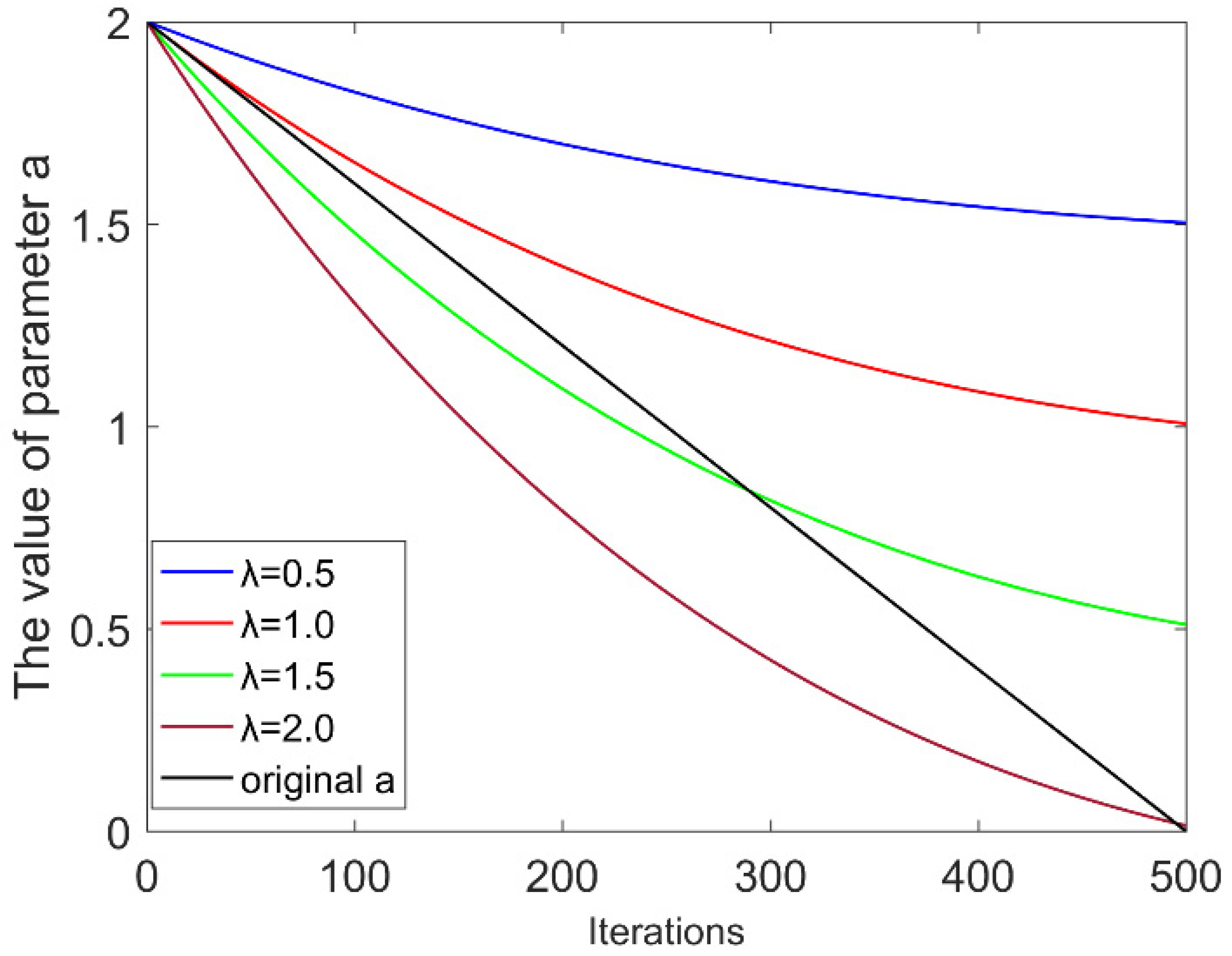
Therefore, a nonlinear control parameter strategy based on exponential functions is proposed in this section. At the early stage of the algorithm update, the descent rate of the proposed parameter $a$ is accelerated, which aims to improve the convergence rate of GWO. In the later stages, the slowdown is performed to enhance the exploitation of the algorithm. The modified convergence factor $a$ can be defined as shown in the Equation (17):

$$a=2-2·\lambda ·\frac{t}{T}·e^{\frac{-0.7t}{T}}$$

(17)

where $t$ is the number of current iterations, $T$ is the maximum number of iterations and $\lambda$ is used to regulate the non-linear declining trend of $a$. To visualize the convergence trend of the proposed parameter $a$, Figure 6 simulates the evolution curve of the parameter $a$ at different $\lambda$ values.

3.5. Discrete Grey Wolf Update Operator (DGUO)

The GWO was first proposed to be applicable for solving continuous optimization problems; nevertheless, FJSP, as a typical discrete combinatorial optimization problem, cannot be directly used by GWO for solving it. For this reason, a reasonable discretization of the coding vector of GWO is required. In this section, a discrete grey wolf update operator (DGUO) is designed, in which each solution corresponds to a grey wolf, and it consists of two parts, i.e., the operation part and the machine part. Its update method is shown in Algorithm 2.

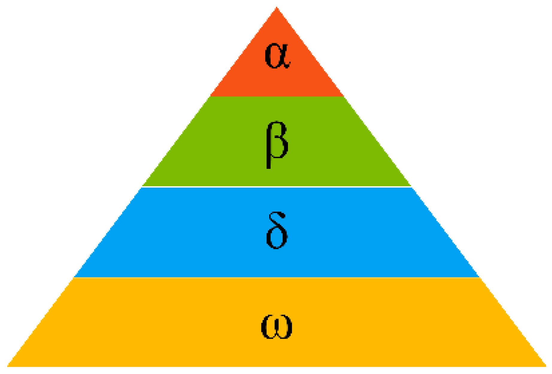
The proposed DGUO has the following three characteristics. According to the social hierarchy of GWO, the wolf packs are divided into leader wolves (α, β, δ) and ordinary wolves (ω), and the role of the leader wolves is to guide the ordinary wolves towards the direction of prey. To distinguish the identity from ordinary wolves, the DGUO is designed with different update methods for these two kinds of wolves. Secondly, in order to enhance individual communication within the population, an intra-population information interoperability strategy was introduced for the update of common wolves, as the movement of ordinary wolves in the search space during the update of GWO was only related to the leader wolves. Finally, a hamming distance-based reception mechanism was adopted to enhance the population diversity and avoid premature convergence of the algorithm.

A two-dimensional space vector schematic is used to explain the update mechanism of DIGWO. The legend has been marked. In Figure 7, (a) and (b) denote the renewal method of ordinary wolves at different stages, respectively. R represents a randomly selected ordinary wolf in the population, and w represents the current ordinary wolf. If |A| < 1, the ordinary wolf is called by the leader wolf to approach it; otherwise, an ordinary wolf is randomly selected in the population to determine the direction and step length of the next movement of the current individual. Figure 7c represents the update of the head wolf, which relies only on its own experience as it moves through the search space. Figure 7d indicates that the generated new generation of individuals is retained not only with reference to the fitness of the individuals, but also selected with a certain probability based on the hamming distance.

Algorithm 2. Overall update process of DGUO
Input: The OS vectors and MS vectors of all grey wolves in $t$ generation, total number of individuals $n$
Output: The OS vectors and MS vectors of all grey wolves in $t+1$ generation
1	All grey Wolf individuals of the $t$ generation were sorted according to the non-decreasing order of makespan
2	$X_{leader}\leftarrow$ The three individuals with the smallest makespan
3	$X_{normal}\leftarrow$ Remaining individual grey wolves
4	for$i=1:n-3$ do
5	$P_1\leftarrow X_{normal}\left(i\right)$
6	if |A| <= 1 then
7	$P_2$ is selected from the $X_{leader}$ by roulette
8	else
9	$P_2$, not the $i$th individual, is randomly selected from within the $X_{normal}$
10	end if
11	$\left\{Of{f}_1,Of{f}_2\right\}\leftarrow IPOXCrossover\left\{P_1,P_2\right\}$
12	$\left\{Of{f}_1,Of{f}_2\right\}\leftarrow MPXMutation\left\{P_1,P_2\right\}$
13	generate a random number $r_2\in \left[0,1\right]$
14	if $r_2>p_{accept}$ then
15	the offspring individual with the smallest makespan is preserved
16	else
17	the offspring individuals further away from $P_2$ is preserved
18	end if
19	end for
20	for$j=1:3$ do
21	the $j$th OS vector was updated by the swap operation based on the critical block
22	generate a random number $r_3\in \left[0,1\right]$
23	if $r_3<0.7$ then
24	the $j$th MS vector was updated using multi-point mutation to randomly select a machine
25	else
26	the $j$th MS vector was updated using multi-point mutation to select the machine with minimum processing time
27	end if
28	end for
29	return the leader wolf and the normal wolf are merged, and the OS and MS of the $t$+1th generation are output

3.5.1. Update Approach Based on Leader Wolf

In order for the leader wolf to better guide the population toward the optimal solution, the update method of the leader wolf will be redesigned. In the design of the update operator for the leader wolf, it combines the coding characteristics of the operation sequence and machine sequence in FJSP, and the strategy of the critical path is also introduced.

The description of the critical path is given below. The critical path is the longest path from the start node to the end node in the feasible scheduling [1]. According to the critical path method in operational research, moving the critical operations in the critical path can improve the solution of FJSP. Therefore, in order to enhance the convergence of the algorithm while reducing the computational cost, the neighborhood structures used are designed based on the movement on the critical path. As shown in Figure 8, all the operations contained in the black line box constitute a complete critical path, where $O_{3,1}$ $O_{4,1}$, $O_{4,2}$, $O_{4,3}$ and $O_{1,3}$ are the critical operations on the critical path. When two or more consecutive critical operations are on the same machine, we call them critical blocks. As shown in Figure 8, $O_{4,3}$ and $O_{1,3}$ are critical blocks.

• Update of operation sequence

The update method of the operation sequence is shown in Figure 9. A new operation sequence is generated by moving the two key operations in the key block [45]. The process of moving needs to satisfy the FJSP constraint that the two operations to be exchanged do not belong to the same job. The rules for the exchange are as follows.

• The swapping operation is performed only on the critical block.
• Only the first two and last two critical operations of the critical block are considered for swapping.
• If there are only two critical operations in the block, the two operations are swapped.

• Update of machine sequence

The machine sequence is updated as shown in Figure 10. A new machine sequence is generated by reselecting machines for the critical operations in the critical path. The specific steps are as follows.

• Determine the number of available machines $m$ in the critical operation $O_{i,j}$.
• If the number of selectable machines is equal to one $\left(m=1\right)$, a new critical operation $O_{i,e}$ is selected; if $m=2$, another machine is selected for replacement; if $m\ge 2$, a machine with the smallest processing time is selected from it for replacement.

3.5.2. Update Approach Based on Ordinary Wolf

In the proposed DGUO, the update of ordinary wolves has the following three features. Firstly, the crossover operator is introduced to achieve the information interaction between the leader wolf and the ordinary wolf, and it can enhance the global search ability of the algorithm. Secondly, the roulette method is used to select one of the three leading wolves for the selection of crossover parents. The significance of using the roulette method is that high-quality information is used more often. Finally, the control parameter $A$ in GWO is retained and improved. 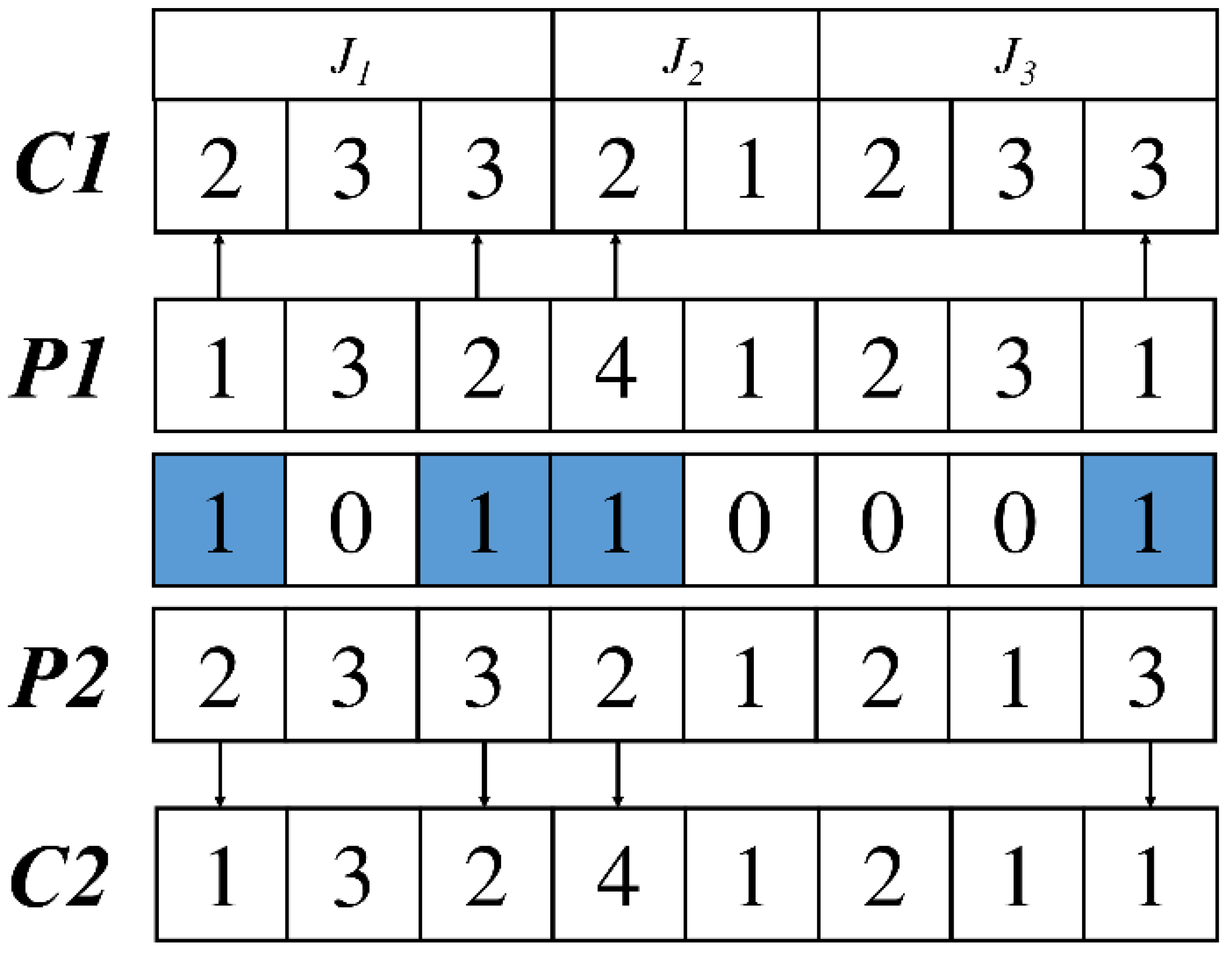If $\left|A\right|<1$, the crossover operation is performed between the current individual and the leader wolf; otherwise, an ordinary wolf is randomly selected from the population to crossover with the current individual. 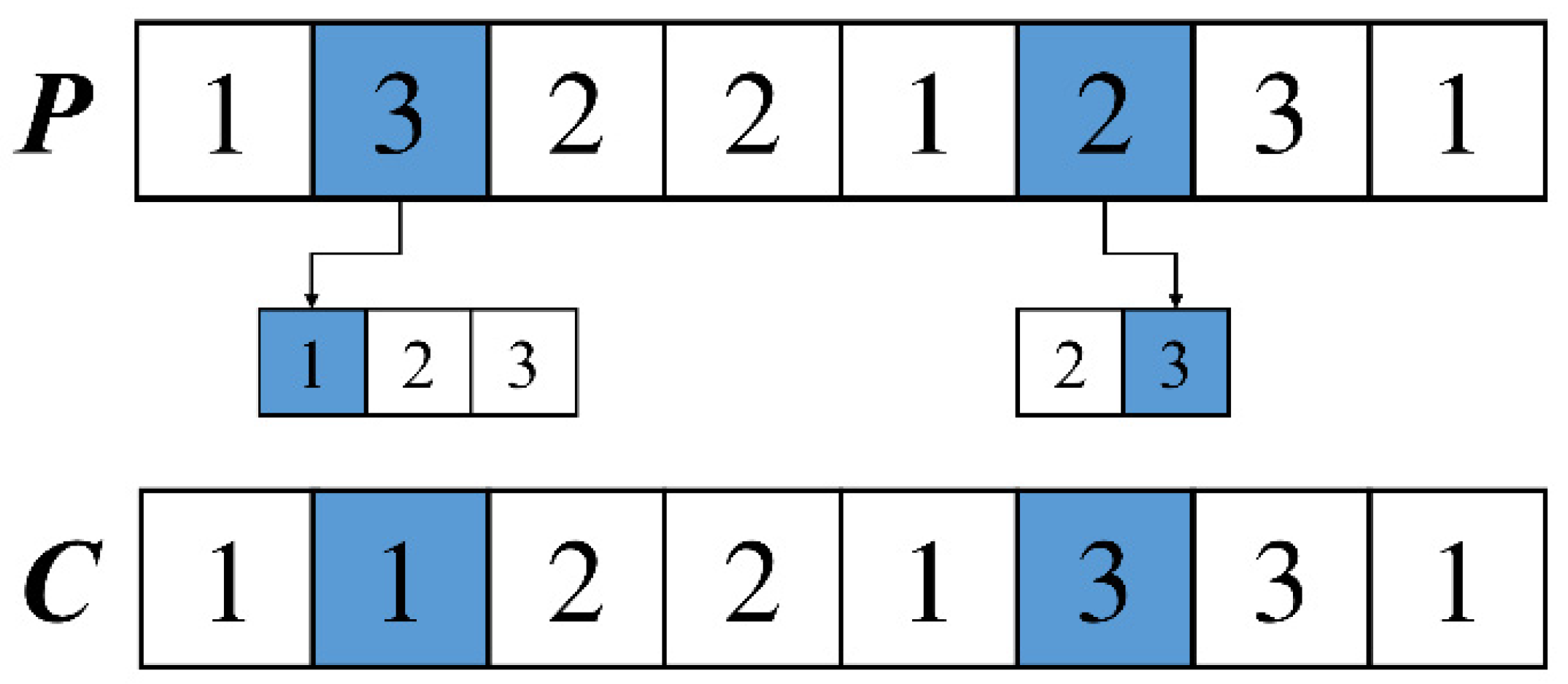The improved priority operation crossover (IPOX) used to operate the sequence update is shown in Figure 11. For machine sequences, the multi-point crossover (MPX) operation is used as shown in Figure 12. These two crossover operators are described below.

• IPOX crossover

Step 1: The job set $J=\left\{J_1,J_2,J_3,\mathrm{I},J_n\right\}$ is randomly divided into two sets, $U_1$ and $U_2$.

Step 2: All elements of the operation sequence of the parent ($P_1)$ which belong to the set $U_1$ are directly retained in Child ($C_1$) in their original positions. Similarly, the elements of the parent $P_2$ which belong to the set $U_2$ are directly retained in $C_2$ and remain in their original positions

Step 3: The vacant places of $C_1$ are filled by the elements of the operation sequence of the parent $P_2$ which belong to the set $U_2$ sequentially. Likewise, the elements belonging to the set $U_1$ in the $P_1$ are filled sequentially to the remaining positions in $C_2$ in order.

• MPX crossover

Step 1: A random array Ra consisting of 0 and 1 is generated and its length is equal to MS.

Step 2: Determine all the positions in RA where the elements are 1 and note them as Index; find the elements at Index position in P1 and P2 and swap them.

Step 3: The remaining elements in P1 and P2 are not moved.

3.5.3. Acceptance Criteria

In order to prevent the population rapidly converging to non-optimal space during the update process, a distance-based reception criterion is proposed. Similar to the role of the control parameter C in GWO, the individual further away from the optimal ones in the search space also has a chance to be retained. Considering the discrete nature of the encoding, the distances are also discretized and called hamming distances in solving the FJSP [45].

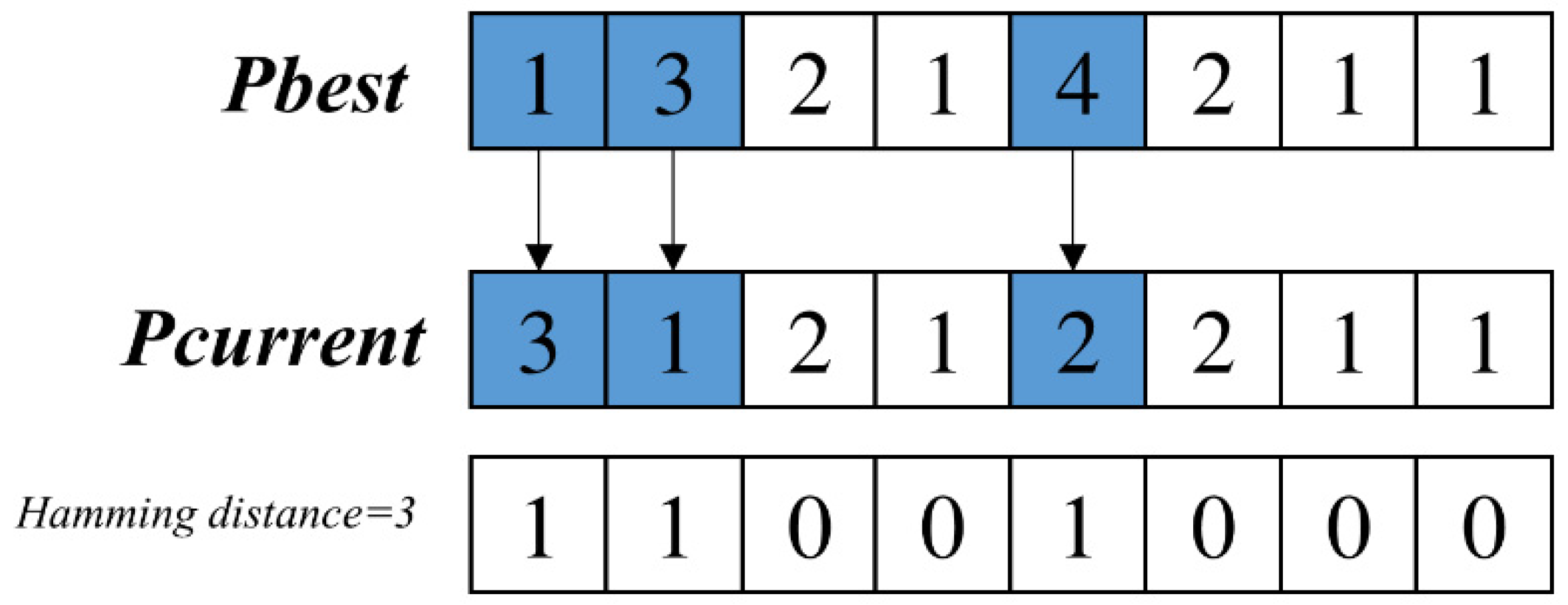
For machine sequences, the hamming distance between two individuals is expressed using the number of unequal elements in the sequence. An example of hamming distance is as follows: if there are two machine sequences in the FJSP solution space, $P_{current}=\left(1,3,2,1,4,2,1,1\right)$ and $P_{best}=\left(3,1,2,1,2,2,1,1\right)$, and if there are three points of inconsistency between the two sequences, the hamming distance is 3. 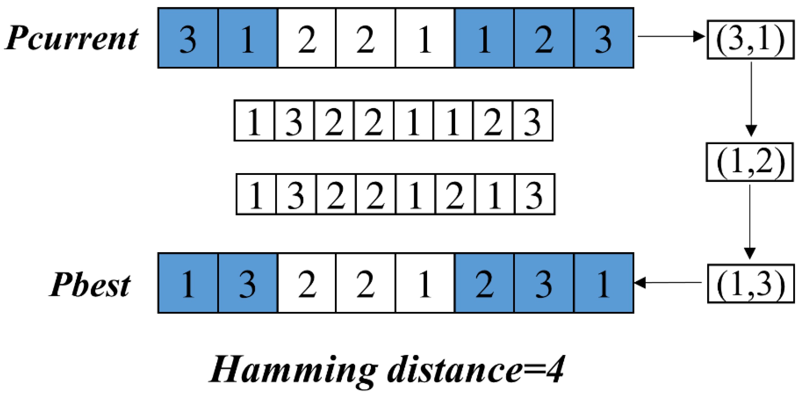This calculation procedure is shown in Figure 13. For operational sequences, the hamming distance between two individuals can be measured by the number of swaps. For example, two operation sequences in FJSP solution space are as follows: $P_{current}=\left(3,1,2,2,1,1,3,2\right)$ and $P_{best}=\left(1,3,2,1,2,1,2,3\right)$; the $P_{current}$ will need four swaps to obtain $P_{best}$, so the hamming distance is 4. This process is shown in Figure 14. The hamming distance between two individuals and the best individual is calculated and compared in turn. If the acceptance probability $p_{accept}$ is satisfied, then the individual is retained using the hamming distance; otherwise, the individual with high fitness in the offspring will be retained.

4. Numerical Analysis

In this section, to investigate the accuracy and stability of the proposed DIGWO, eight benchmark test functions are employed in the experiments with dimensions set to D = 30, 50 and 100. As shown in

Table 5. Details of benchmark functions.

Name	Functions	C	Range	fmin
Sphere	$f_1\left(x\right)={\sum }_{i=1}^n{x}_i^2$	US	[−100, 100]	0
Sumsquare	$f_2\left(x\right)={\sum }_{i=1}^{n}i{x}_i^2$	US	[−10, 10]	0
Schwefel2.21	$f_3\left(x\right)=\underset{i}{max}\{\left|x_i\right|,1⩽i⩽n\}$	UN	[−100, 100]	0
Schwefel2.22	$f_4\left(x\right)={\sum }_{i-1}^n\left|x_i\right|+{\Pi }_{i=1}^n\left|x_i\right|$	UN	[−10, 10]	0
Rosenbrock	$f_5\left(x\right)={\sum }_{i=1}^{n-1}[100{(x_{i+1}-x_i^2)}^2+{(x_i-1)}^2]$	UN	[−5, 10]	0
Rastrigin	$F_6\left(x\right)={\sum }_{i=1}^n[x_i^2-10\cos (2𝜋x_i)+10]$	MS	[−5.12, 5.12]	0
Ackley	$F_7\left(x\right)=-20\exp (-0.2\sqrt{\frac{1}{n}{\sum }_{i=1}^n{x}_i^2})-\exp (\frac{1}{n}{\sum }_{i=1}^n\cos (2𝜋x_i))+20+e$	MN	[−32, 32]	0
Levy	$F_{13}\left(x\right)={\sum }_{i=1}^n{(x_i-1)}^2[1+{\sin }^2(3𝜋x_i+1)]+|x_n-1|[1+{\sin }^2(3𝜋x_n)]$	MN	[−10, 10]	0

, the functions are characterized by U, M, S and N, corresponding to unimodal, multimodal, separable and non-separable. The proposed DIGWO was coded in MATLAB 2016a software on an Intel 3.80 GHz Pentium Gold processor with 8 Gb RAM on a Win10 operating system. In the later experiments for solving FJSP, this same operating environment is used.

The unimodal function has only one optimal solution, Io it is used to verify the exploitation capability of the algorithm. In contrast, the multimodal function has multiple local optima and is therefore used to test the exploration capability of the algorithm. The purpose of setting multiple dimensions is to test the stability of the algorithms’ performance on problems of different complexity. To verify the effectiveness and superiority of the algorithms, there are five metaheuristic algorithms which have been proposed in recent years used for comparison: GWO, PSO, MFO, SSA, SCA and Jaya [35,57,58,59,60,61]. In order to ensure fairness during the experiment, the population size was set to 30, and the maximum number of iterations was set to 3000, 5000 and 10,000 according to the order of the dimensionality (D = 30, 50, 100). All other parameters of the algorithms involved in the comparison were set according to the relevant literature. Each algorithm was run 30 times independently on each benchmark function.

Table 6. Comparison of results for 30-dimension benchmark functions.

Algorithm		f1	f2	f3	f4	f5	f6	f7	f8
DIGWO	Mean	2.60 × 10−267	6.28 × 10−271	5.05 ×10−65	4.73 × 10−157	2.68 × 101	0	7.82 × 10−15	3.61
	Std	0	0	1.63 ×10−64	7.25 × 10−157	1.04	0	0	2.07
PSO	Mean	4.17 × 10−22	1.07 × 10−19	1.58 × 10−1	5.52 × 10−11	3.25 × 101	3.53 × 101	1.54 × 10−12	1.10 × 10−2
	Std	1.63 × 10−21	3.29 × 10−19	6.30× 10−2	1.21 × 10−10	2.87 × 101	1.00 × 101	3.87 × 10−12	3.38 × 10−2
	Sig	+	+	+	+	=	+	+	-
MFO	Mean	2.00 × 103	2.50 × 101	6.77 × 101	4.00 × 101	1.36 × 105	1.54 × 102	1.53 × 101	8.72 × 101
	Std	4.10 × 103	4.44 × 101	8.65	2.41 × 101	6.57 × 104	3.41 × 101	6.70	8.90 × 101
	Sig	+	+	+	+	+	+	+	=
SSA	Mean	6.44 × 10−9	6.74 × 10−11	3.20	6.91 × 10−1	5.14 × 101	6.99 × 101	1.90	4.85× 10−2
	Std	1.29 × 10−9	1.30 × 10−11	2.67	8.96 × 10−1	3.32 × 101	1.11 × 101	8.84 × 10−1	7.32× 10−2
	Sig	+	+	+	+	+	+	+	-
SCA	Mean	1.76 × 10−11	6.44 × 10−13	3.12	4.27 × 10−17	2.78 × 101	2.87 × 10−2	9.64	2.03 × 101
	Std	7.85 × 10−11	2.87 × 10−12	5.25	9.67 × 10−17	3.15 × 10−1	1.28 × 10−1	9.80	1.64
	Sig	+	+	+	+	+	+	+	+
Jaya	Mean	1.50 × 101	2.60 × 10−1	4.93E-01	3.08 × 101	3.74 × 10−2	7.94 × 101	7.66	6.86 × 10−1
	Std	1.31 × 101	6.87	3.10E-01	1.28 × 101	3.04 × 10−2	3.58 × 101	6.87	6.54 × 10−1
	Sig	+	+	+	+	-	+	+	+
GWO	Mean	3.55 × 10−226	1.25 × 10−228	8.17 × 10−58	1.18 × 10−130	2.74 × 101	0	7.99 × 10−15	5.92
	Std	0	0	3.30 × 10−57	3.63 × 10−130	1.34	0	7.94 × 10−16	1.43
	Sig	+	+	+	+	=	=	=	+

,

Table 7. Comparison of results for 50-dimension benchmark functions.

Algorithm		f1	f2	f3	f4	f5	f6	f7	f8
DIGWO	Mean	0	0	9.22 × 10−74	1.33 × 10−200	4.69 × 101	0	8.88 × 10−15	1.34 × 101
	Std	0	0	2.35 × 10−73	0	8.03 × 10−1	0	2.27 × 10−15	2.42
PSO	Mean	4.85 × 10−16	1.78 × 10−14	1.07	1.49 × 10−6	8.13 × 101	9.17 × 101	3.73 × 10−9	2.20 × 10−2
	Std	9.50 × 10−16	7.89 × 10−14	2.00 × 10−1	5.56 × 10−6	3.89 × 101	2.75 × 101	6.51 × 10−9	4.51 × 10−2
	Sig	+	+	+	+	+	+	+	-
MFO	Mean	7.00 × 103	9.50 × 101	8.07 × 101	6.20 × 101	3.10 × 105	2.72 × 102	1.97 × 101	1.44 × 102
	Std	8.01 × 103	8.87 × 101	5.71	2.84 × 101	1.66 × 105	4.19 × 101	4.18 × 10−1	1.19 × 102
	Sig	+	+	+	+	+	+	+	+
SSA	Mean	1.76 × 10−8	1.85 × 10−10	1.17 × 101	1.72	7.14 × 101	1.07 × 102	2.36	8.67 × 10−2
	Std	1.99 × 10−9	2.80 × 10−11	3.61	1.77	3.44 × 101	2.71 × 101	5.29 × 10−1	2.18 × 10−1
	Sig	+	+	+	+	=	+	+	+
SCA	Mean	7.21 × 10−6	5.47 × 10−8	2.93 × 101	4.21 × 10−15	4.84 × 101	1.09 × 101	1.55 × 101	4.31 × 101
	Std	2.52 × 10−5	1.85 × 10−7	9.13	1.57 × 10−14	4.77 × 10−1	2.41 × 101	8.17	2.26
	Sig	+	+	+	+	+	+	+	+
Jaya	Mean	6.03 × 103	1.96 × 101	6.25 × 10−1	3.86 × 101	1.54 × 10−2	1.44 × 102	3.36	7.48 × 101
	Std	5.48 × 103	4.14 × 101	2.13 × 10−1	2.01 × 101	2.24 × 10−2	5.87 × 101	4.85	1.18 × 102
	Sig	+	+	+	+	-	+	+	=
GWO	Mean	4.20 × 10−283	4.06 × 10−285	5.57 × 10−64	3.43 × 10−165	4.64 × 101	0	1.03 × 10−14	1.74 × 101
	Std	0	0	1.57 × 10−63	0	1.03	0	2.89 × 10−15	3.19
	Sig	+	+	+	+	=	=	=	+

and

Table 8. Comparison of results for 100-dimension benchmark functions.

Algorithm		f1	f2	f3	f4	f5	f6	f7	f8
DIGWO	Mean	0	0	2.06 × 10−85	4.51 × 10−288	9.69 × 101	0	1.37 × 10−14	5.35 × 101
	Std	0	0	7.84 × 10−85	0	8.96 × 10−1	0	2.00 × 10−15	3.47
PSO	Mean	4.43 × 10−9	1.24 × 10−9	3.01	5.21 × 10−4	2.01 × 102	2.73 × 102	6.08 × 10−2	1.15 × 10−1
	Std	1.25 × 10−8	2.02 × 10−9	2.83 × 10−1	9.67 × 10−4	6.31 × 101	5.08 × 101	2.71 × 10−1	2.38 × 10−1
	Sig	+	+	+	+	+	+	+	-
MFO	Mean	1.57 × 104	2.35 × 102	9.25 × 101	1.37 × 102	8.71 × 105	6.32 × 102	1.98 × 101	4.46 × 102
	Std	9.11 × 103	1.60 × 102	2.05	4.62 × 101	4.47 × 105	8.99 × 101	2.97 × 10−1	3.70 × 102
	Sig	+	+	+	+	+	+	+	+
SSA	Mean	7.02 × 10−8	7.13 × 10−10	2.25 × 101	6.55	1.75 × 102	2.07 × 102	3.64	4.64 × 101
	Std	7.93 × 10−9	7.63 × 10−11	3.78	2.99	6.15 × 101	4.81 × 101	6.24 × 10−1	9.53 × 101
	Sig	+	+	+	+	+	+	+	-
SCA	Mean	2.63 × 101	2.67 × 10−1	6.85 × 101	8.59 × 10−11	4.09 × 103	1.22 × 102	1.93 × 101	1.18 × 102
	Std	5.37 × 101	5.58 × 10−1	5.41	3.31 × 10−10	3.45 × 103	6.83 × 101	4.63	1.92 × 101
	Sig	+	+	+	+	+	+	+	+
Jaya	Mean	3.45 × 104	2.40 × 102	3.21 × 10−1	1.46 × 102	5.47 × 10−2	3.13 × 102	5.00	3.17 × 102
	Std	3.41 × 104	1.91 × 102	1.59 × 10−1	5.09 × 101	3.40 × 10−2	9.82 × 101	4.83	4.05 × 102
	Sig	+	+	+	+	+	+	+	=
GWO	Mean	0	0	4.76 × 10−61	3.96 × 10−232	9.69 × 101	0	1.51 × 10−14	6.26 × 101
	Std	0	0	2.13 × 10−60	0	1.03	0	2.13 × 10−15	3.63
	Sig	=	=	+	+	=	=	+	+

give the running results of the comparison algorithm obtained in the test functions of 30, 50 and 100 dimensions. The mean (Mean) and standard deviation (Std) obtained from the run results are used as evaluation metrics to represent the performance of the algorithm. The best results are bolded. To test the significance difference between the algorithms, the Wilcoxon signed rank test with a significance level of 0.05 is used. The statistical result Sig is marked as “$+/=/-$”, which means DIGWO is better than, equal to or inferior to the algorithms involved in the comparison.

From Table 6, Table 7 and Table 8, it can be concluded that DIGWO has greater convergence and stability on most problems. In particular, the proposed algorithm achieves better results on all problems compared to the original GWO. Combining the statistical results of standard deviation and Wilcoxon test results, DIGWO significantly outperforms other algorithms on problems, excluding f5 and f8, and is robust on problems with different dimensions. The results of the statistical significance tests obtained by the proposed DIGWO and comparison algorithms in different dimensions are discussed below. In the comparison with PSO, DIGWO has 20 results that outperform PSO, one result that is not significantly different from PSO and three results that are worse than PSO. In the comparison with MFO, DIGWO had 23 results superior to MFO and one result not significantly different from MFO. In the comparison with SSA, DIGWO had 21 results better than SSA, one result not significantly different from SSA and two results worse than SSA. In the comparison with SCA, all results of DIGWO were better than SCA. In the comparison with Jaya, DIGWO had 20 results better than Jaya, two results not significantly different from Jaya and two results worse than Jaya. In the comparison with GWO, 14 results of DIGWO were better than GWO, and 10 results were not significantly different from GWO.

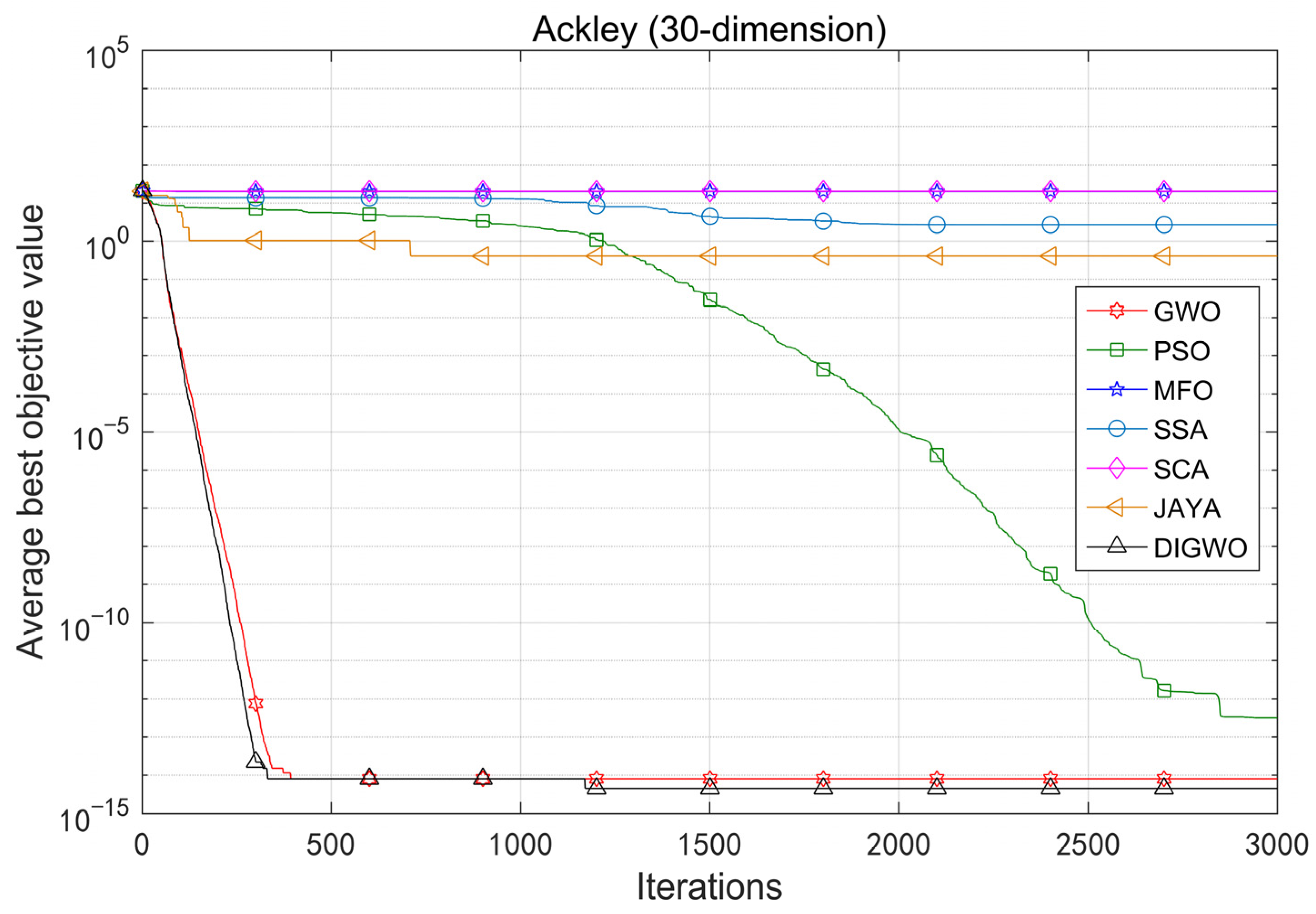
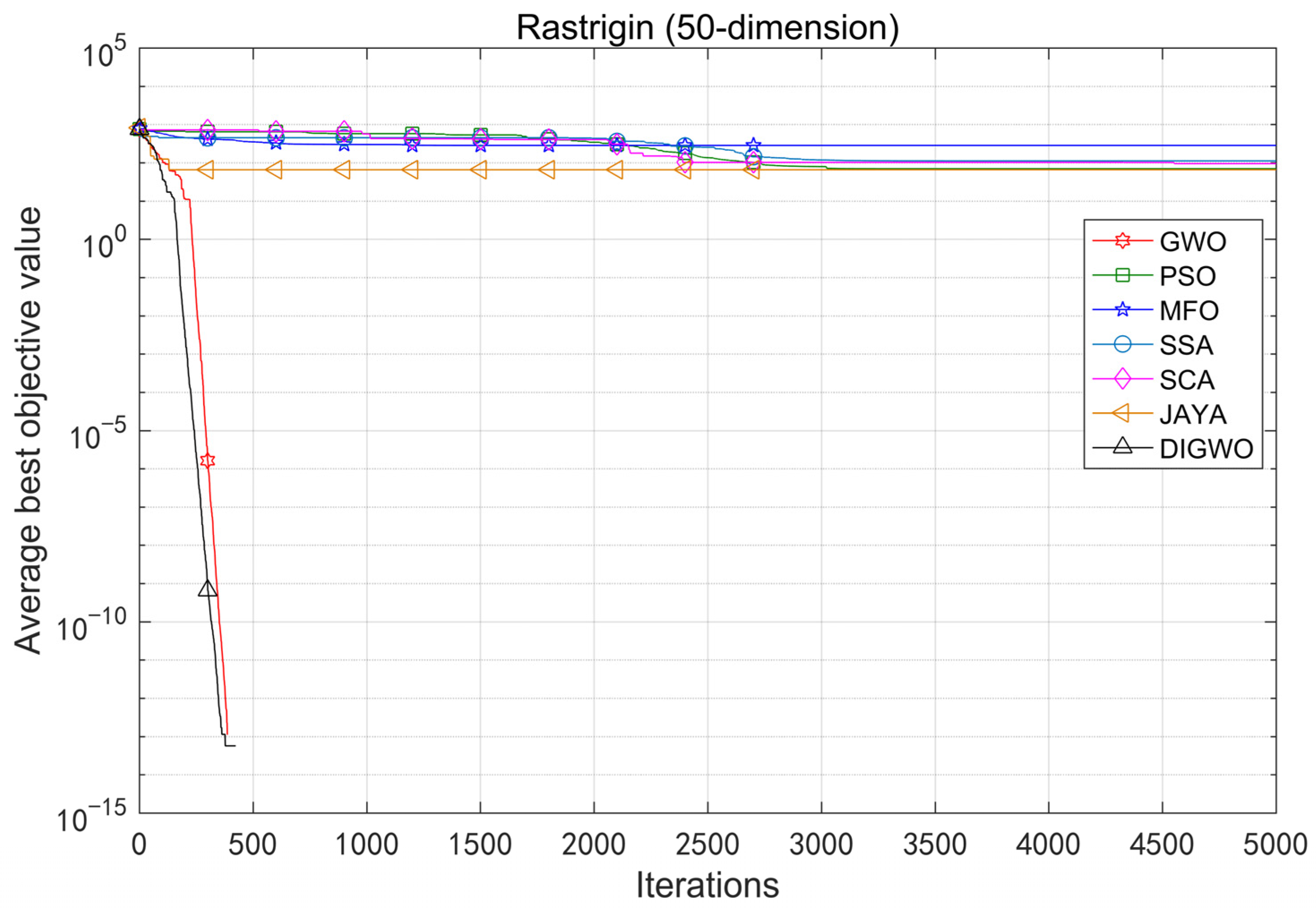
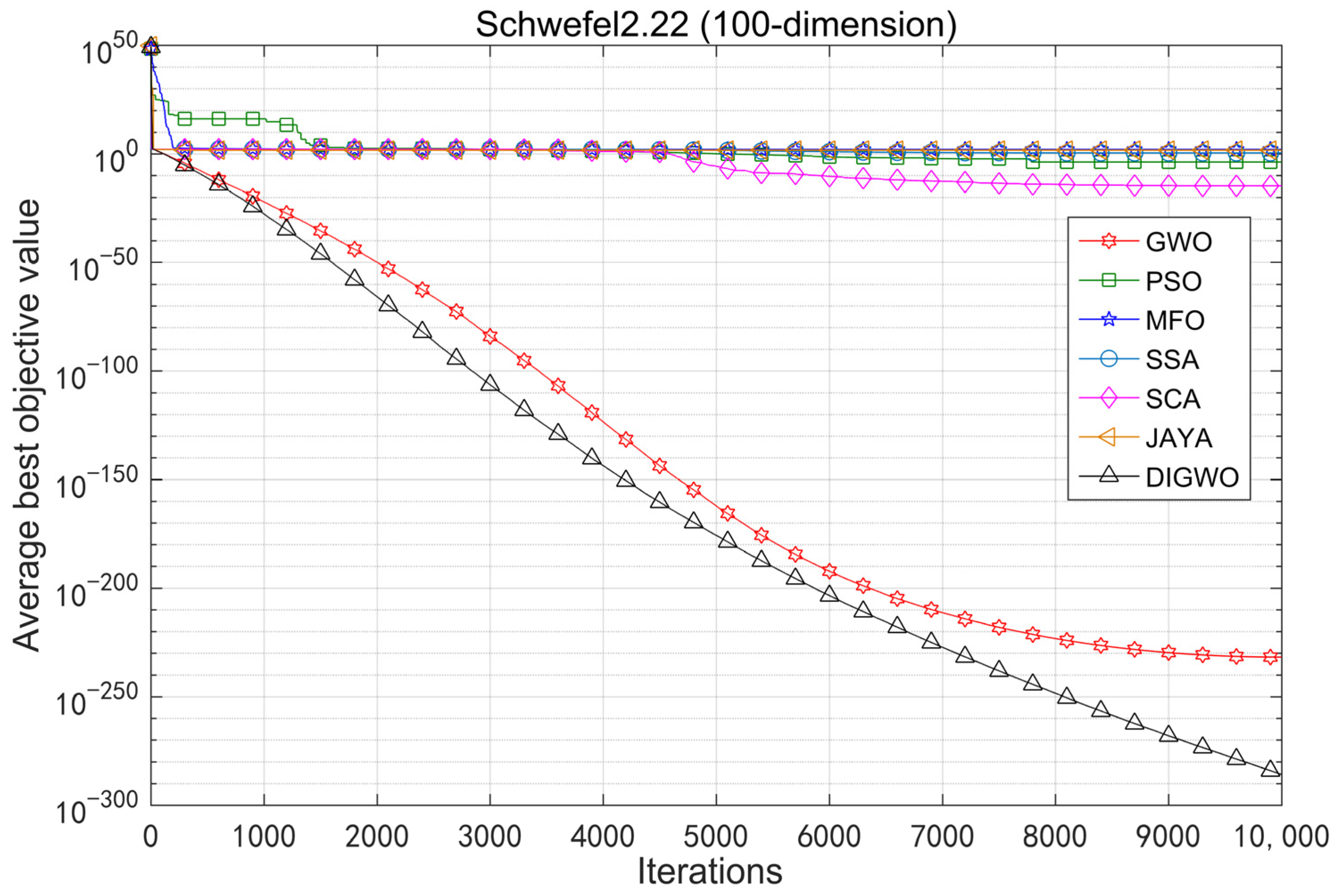
To further investigate the performance of DIGWO, some representative test functions are selected to analyze the convergence trends of all the algorithms involved in the comparison. The convergence curves are shown in Figure 15, Figure 16 and Figure 17. The convergence curves of the multimodal benchmark functions are shown in Figure 15 and Figure 16, and the convergence curves of the unimodal benchmark test functions are shown in Figure 17. It can be observed that the proposed algorithm outperforms other algorithms in terms of convergence speed and accuracy. This also shows the effectiveness of the proposed improvement strategy in DIGWO. Figure 15 and Figure 17 show that the results of the algorithm can still be improved even in the middle and late stages of the iteration, which further indicates the improved development capability. The convergence curve in Figure 16 shows that DIGWO can converge to the theoretical optimum in the shortest time, which also verifies the efficient global search capability of DIGWO. In conclusion, the overall search performance of DIGWO based on the chaotic mapping strategy and adaptive convergence factor is effective.

5. Simulation of FJSP Based on DIGWO

5.1. Notation

The following notations are used in this section to evaluate algorithms or problems, and the definitions of these notations are explained below.

LB: Lower bound of the makespan values found so far.

Best: Best makespan in several independent runs.

WL: Best critical machine load achieved from several independent runs.

Avg: The average makespan obtained from several independent runs.

T_cpu: Computation time required for several independent runs to obtain the best makespan (seconds).

T(AV): The average computation time obtained by the current algorithm for all problems in the test problem set.

RE: The relative error between the optimal makespan obtained by the current algorithm and the LB, given by Equation (18).

$$\mathrm{RE}=\frac{\mathrm{Best}-\mathrm{LB}}{\mathrm{LB}}$$

(18)

MRE: The average RE obtained by the current algorithm for all problems of the test problem set.

RPI: Relative percentage increase, given by Formula (19).

$$\mathrm{RPI}=\frac{{\mathrm{MK}}_i-{\mathrm{MK}}_b}{{\mathrm{MK}}_b}$$

(19)

where ${\mathrm{MK}}_i$ is the best makespan obtained by the ith comparison algorithm, and ${\mathrm{MK}}_b$ denotes the best makespan among all the algorithms involved in the comparison.

5.2. Description of Test Examples

In order to test the performance of the algorithm, international benchmark arithmetic cases are used. The well-known experimental sets include KCdata, BRdata and Fdata.

BRdata is offered by Brandimarte and includes 10 problems: MK01–MK10, ranging in size from 10 jobs to 20 jobs, 4 machines to 15 machines, with medium flexibility and a range of F 0.15–0.35 [15].

KCdata is provided by Kacem, which contains five problems: Kacem01–Kacem05, ranging in size from 4 jobs and 5 machines to 15 jobs and 10 machines, and all four problems are total flexible job shop scheduling problems, except Kacem02 [62].

Fdata is provided by Fattahi et al. which contains 20 problems, namely SFJS01–SFJS10 and MFJS01–MFJS10. The size of the problems ranges from two jobs and two machines to nine jobs and eight machines [63].

The existing literature does not contain test problems for large-scale FJSP; therefore, a dataset is proposed and named YAdata, which contains 12 test problems. The details of these problems are given in

Table 9. Information about the generated LSFJSP.

Problem	Job	Machine	Operation	F	Time
YA01	100	60	10–20	0.2	5–20
YA02				0.3
YA03				0.5
YA04	100	60	10–20	0.2	5–20
YA05				0.3
YA06				0.5
YA07	100	60	10–20	0.2	5–20
YA08				0.3
YA09				0.5
YA10	100	60	10–20	0.2	5–20
YA11				0.3
YA12				0.5

, where Job denotes the number of jobs, Machine means the number of machines, Operation represents the number of operations contained in each job, F denotes the ratio of the number of machines that can be selected for each operation to the total number of machines and Time denotes the range of processing time values.

5.3. Parameter Analysis

The parameter configuration affects the performance of the algorithm in solving the problem. In the proposed DIGWO, the parameters that perform best in the same environment are obtained through experimental tests. Depending on the size of the test problem, the total population of DIGWO is set to 50 when testing three international benchmark FJSPs, namely BRdata, KCdata and Fdata. In testing the large-scale FJSP, namely YAdata, the total population is set to 50. The number of generations is set to 200.

The following sensitivity tests were performed for the key parameters used in the proposed DIGWO. For fairness, Mk04 was used as the test problem and the Avg obtained from 20 independent runs was collected to evaluate the performance. The parameter levels are as follows: $\lambda =\left\{0.5,1.0,1.5,2.0\right\}$ and $p_{accept}=\left\{0.1,0.2,0.3,0.4\right\}$. The experimental results obtained with different combinations of parameters are given in

Table 10. Sensitivity analysis of key parameters.

DIGWO	$\mathit{\lambda } = 0.5$	$\mathit{\lambda } = 1.0$	$\mathit{\lambda } = 1.5$	$\mathit{\lambda } = 2.0$
$p_{accept}$ = 0.1	64.55	64.20	64.05	65.00
$p_{accept}$ = 0.2	64.80	65.05	65.70	65.10
$p_{accept}$ = 0.3	64.60	65.45	65.60	66.20
$p_{accept}$ = 0.4	65.20	65.60	65.00	65.05

. The comprehensive observation shows that the best performance of the algorithm is obtained when $\lambda$ = 1.5 and $p_{accept}$ = 0.1.

5.4. Analysis of the Effectiveness of the Proposed Strategy

5.4.1. Validation of the DGUO Strategy

To verify the effectiveness of the DGUO proposed in this paper, the performance of GWO-1 and GWO-2 is compared. GWO-1 is the basic grey wolf optimization algorithm and it uses the conversion mechanism which is already available in the literature [41]. The GWO-2 is a discrete algorithm that uses the DGUO strategy proposed in this paper. Other than that, none of the other improvement strategies proposed in this paper were used during the experiments. The performance of these two algorithms was evaluated on BRdata considering the same parameters. To ensure fairness during the experiments, the results after 20 independent runs are shown in

Table 11. Comparison of proposed updating methods.

Instance	GWO-1				GWO-2
	Best	WL	Avg	Tcpu	Best	Best	WL	Avg	Tcpu
MK01	44	42	47.85	9.307	42	41	36	42.35	7.043
MK02	37	36	39.5	9.890	30	28	28	28.9	7.233
MK03	232	213	245.6	23.62	204	204	204	204.45	14.52
MK04	76	73	80.75	14.60	73	66	66	70.4	10.52
MK05	189	187	196.3	16.79	176	173	173	176.7	11.25
MK06	100	88	107.1	23.59	94	77	74	81.1	14.98
MK07	177	171	185.85	16.40	163	145	145	149.75	11.47
MK08	543	542	567.2	33.16	523	523	523	524.6	21.90
MK09	412	380	431.5	36.72	377	337	337	350.25	22.27
MK10	342	310	357.45	37.53	301	252	244	265.1	22.33

.

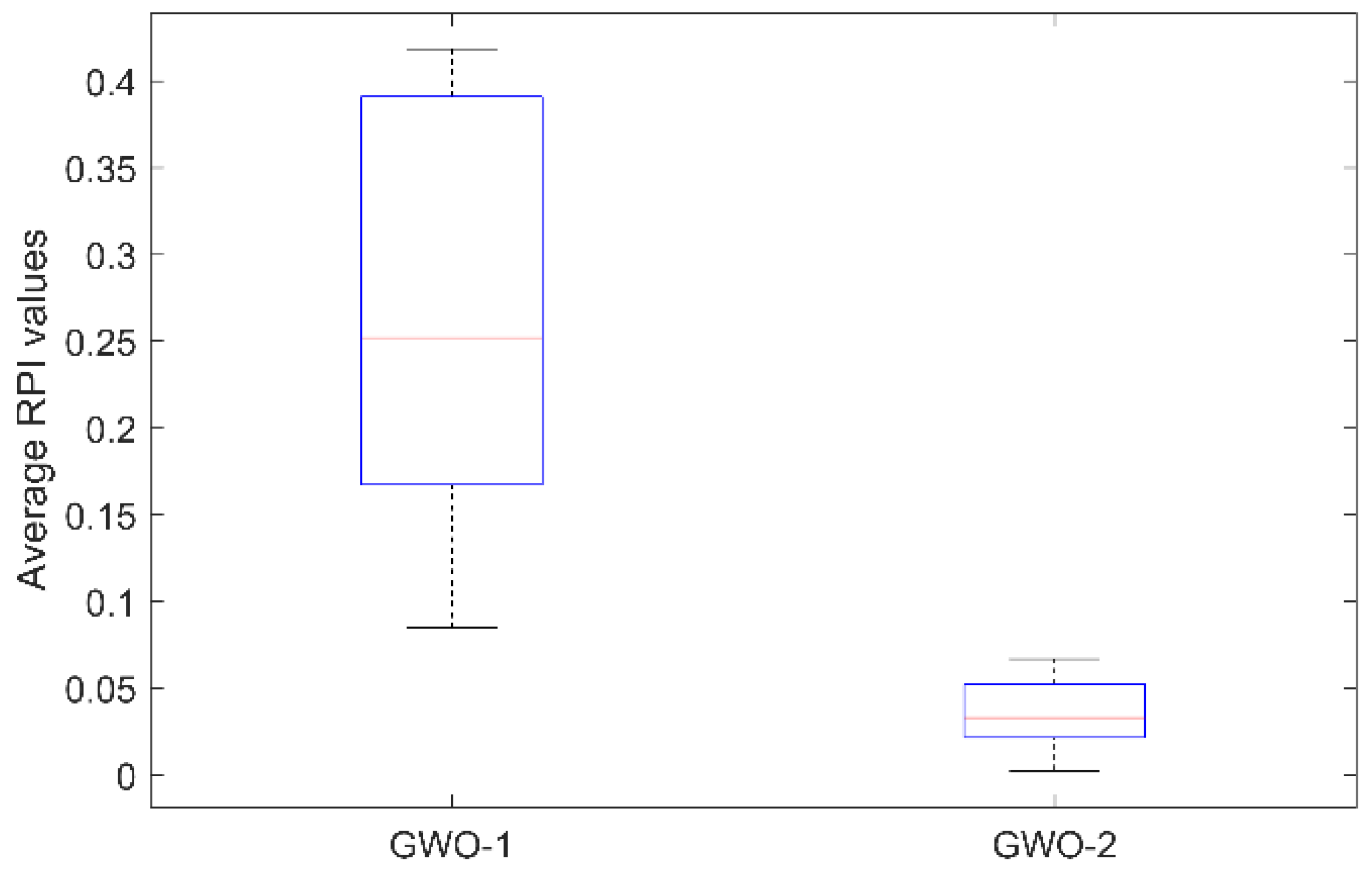
As can be seen from Table 11, GWO-2 always outperforms or equals GWO-1 for both makespan and critical machine load metrics. The average computation time for all instances of GWO-2 on BRdata is 14.3516. This value is smaller than the GWO-1. The resulting advantage in computation time can be attributed to the fact that the algorithm uses a transformation mechanism that requires additional computations at each generation. A comparative box plot of the average RPI values is given in Figure 18, and it can be clearly seen that GWO-2 has the smaller box block and is positioned downwards, which means that the algorithm is highly robust and convergent.

To further analyze the performance, Figure 19 shows the convergence curves of the two compared algorithms on MK08. It can be found that GWO-2 converges to the optimal makespan in 61 generations, and GWO-1 converges in 163 generations. Therefore, the improved discrete update mechanism can enhance the convergence speed of the algorithm.

5.4.2. Validation of Initialization Strategy

In order to test the performance of the hybrid initialization strategy mentioned in Section 3.3, this section includes the test of the two comparison algorithms, DIGWO-RI and DIGWO. It should be noted that the initial populations of DIGWO-RI are generated randomly. To ensure fairness during the experiments, the same components and all parameters were set identically, and the results after 20 independent runs are shown in

Table 12. Comparison of proposed initialization strategy.

Instance	DIGWO-RI				DIGWO
	Best	WL	Avg	Tcpu	Best	WL	Avg	Tcpu
MK01	40	36	41.4	7.806	40	36	41.3	7.159
MK02	27	27	27.5	11.13	26	26	27.1	8.195
MK03	204	204	204	15.21	204	204	204	15.42
MK04	60	60	64.95	10.32	60	60	63.8	10.65
MK05	173	173	176.2	11.28	173	173	173.5	11.23
MK06	65	62	69.2	16.52	62	58	63.7	16.93
MK07	145	145	149.7	11.89	140	140	142.2	12.04
MK08	523	523	523	21.71	523	523	523	21.79
MK09	311	307	323.4	23.25	307	299	314.7	22.95
MK10	226	222	235.7	24.07	211	206	216.5	24.38

.

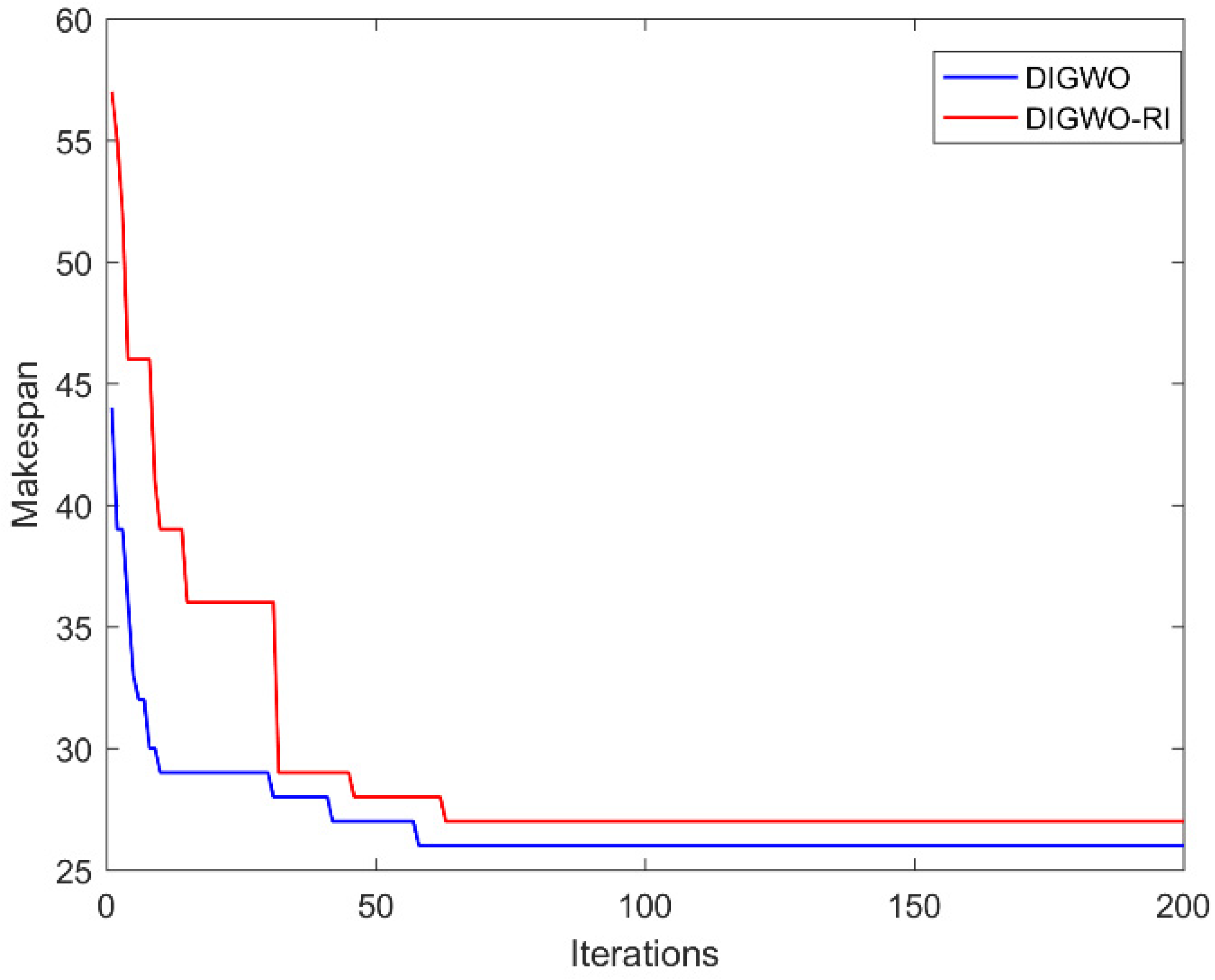
Combining Table 12 and Figure 20, it can be seen that the proposed DIGWO has better makespan and critical machine load than DIGWO-RI on all instances of BRdata. This demonstrates that combining heuristic rules with chaotic mapping strategies can provide suitable initial populations. The optimal convergence curves obtained by the comparison algorithms on MK02 are given in Figure 21. It is observed that DIGWO converges to the optimal makespan in 58 iterations, while DIGWO-RI converges in 63 generations. Additionally, it should be noted that DIGWO is much better than the comparison algorithm in the results of the first iteration. Consequently, the improved initialization strategy proposed in this paper can generate high-quality initial solutions and enable the algorithm to converge to the optimal solution earlier.

5.5. Comparison with Other Algorithms

In this section, DIGWO is compared with algorithms proposed in recent years, and “Best” is the primary metric considered in the process of comparison. To further analyze the overall performance of the algorithm, MRE is also used as a participating comparative performance metric. Considering the differences in programming platforms, processor speed and coding skills used by the algorithms involved in the comparison, the original programming environment and programming platform are given accordingly in the comparison process, and T_cpu and T(AV) are used as comparison metrics. In the following, KCdata, BRdata and Fdata are used as experimental test problems and the comparison results are shown.

5.5.1. Comparison Results in KCdata

In this section, KCdata is used to test the performance of the proposed algorithm, and the results of the proposed algorithm are compared with recent studies IWOA, GATS+HM, HDFA and IACO [24,41,45,64]. To ensure fairness in the experimental process, the results of 20 independent runs are shown in

Table 13. Comparison of DIGWO with other algorithms for KCdata.

Instance	$\mathit{n}\times \mathit{m}$	IWOA a		GATS+HM b		HDFA c		IACO d		HGWO e		DIWO
		Best	Tcpu	Best	Tcpu	Best	Tcpu	Best	Tcpu	Best	Tcpu	Best	WL	Avg	Tcpu
Kacem01	4 × 5	11	1.8	11	0.05	11	0.13	11	0.51	11	5.6	11	11	11	3.49
Kacem02	8 × 8	14	2.9	14	0.36	14	3.53	14	3.53	14	14.8	14	14	14	4.59
Kacem03	10 × 7	13	3.3	11	0.73	11	2.63	11	3.26	11	16.8	11	11	11	4.74
Kacem04	10 × 10	7	4.1	7	1.51	7	3.36	7	4.45	7	17.5	7	6	7	5.27
Kacem05	15 × 10	14	7.9	11	29.7	11	19.3	11	4.86	13	40.4	11	11	11.3	8.34
T(AV)		4.0		6.5		5.8		3.3		19.0			5.29

^a The CPU time on an Intel 1.80 GHz Core i5-8250 processor with 8 Gb RAM in MATLAB 2016a. ^b The CPU time on an Intel 2.1 GHz processor with 3 Gb RAM in Java. ^c The CPU time on an Intel 2.0 GHz Core 2 Duo processor with 4 Gb RAM in C++. ^d No system data provided by authors. ^e The CPU time on an Intel 1.80 GHz Core i5-8250 processor with 8 Gb RAM in MATLAB 2016a.

. From the results in Table 13, it can be found that the best makespan obtained by the proposed DIGWO is always better than or equal to the other five compared algorithms, and the average computation time is shorter. In summary, the proposed DIGWO has more competitive advantages in terms of the accuracy of the search and convergence speed. Figure 22 shows the optimal resultant Gantt chart (makespan = 11) obtained by the proposed algorithm in Kacem05.

5.5.2. Comparison Results in BRdata

In this section, BRdata is used to test the performance of the proposed algorithm, and the results of the proposed DIGWO are compared with those of recent studies IWOA, HGWO, PGDHS, GWO and SLGA [21,41,51,65,66]. To eliminate randomness in the experimental process, the results of 20 independent runs are shown in

Table 14. Comparison of DIGWO with other algorithms for BRdata.

Instance	n × m	LB	IWOA a		HGWO b		PGDHS c		GWO d		SLGA e		DIGWO
			Best	Tcpu	Best	Tcpu	Best	Tcpu	Best	Tcpu	Best	Tcpu	Best	WL	Avg	Tcpu
MK01	10 × 6	40	40	8.2	40	36.3	40	5.3	40	64.6	40	27.6	40	36	41.3	7.159
MK02	10 × 6	26	26	8.8	29	38.7	26	5.4	29	70.0	27	29.1	26	26	27.1	8.195
MK03	15 × 8	204	204	31.3	204	165.8	204	24.1	204	377.6	204	112.6	204	204	204	15.42
MK04	15 × 8	60	60	15.7	65	75.9	62	14.7	64	218.2	60	63.2	60	60	63.8	10.65
MK05	15 × 4	172	175	21.2	175	95.7	173	9.0	175	131.4	172	60.4	173	173	173.5	11.23
MK06	10 × 15	57	63	30.5	79	168.6	62	25.8	69	480.7	69	72.8	62	58	63.7	16.93
MK07	20 × 5	139	144	24.7	149	92.1	140	13.9	147	213.4	144	57.8	140	140	142.2	12.04
MK08	20 × 10	523	523	89.2	523	340.8	523	53.6	523	1026.2	523	521.7	523	523	523	21.79
MK09	20 × 10	307	339	121.4	325	378.9	307	62.4	322	1123.8	320	552.5	307	299	314.7	22.95
MK10	20 × 15	189	242	96.7	253	388.5	211	79.0	249	1744.3	254	1335.2	211	206	216.5	24.38
T(AV)			44.8		178.1		29.3		545.0		283.3		15.07
MRE			0.0543		0.1071		0.0250		0.0834		0.0671		0.0217

^a The CPU time on an Intel 1.80 GHz Core i5-8250 processor with 8 Gb RAM in MATLAB 2016a. ^b,d The CPU time on 2 Gb RAM in FORTRAN. ^c The CPU time on an Intel 2.8 GHz PC with 1 GB RAM in C++. ^e The CPU time on an Intel 1.80 GHz Core i5-4590 processor with 8 Gb RAM in MATLAB 2018a.

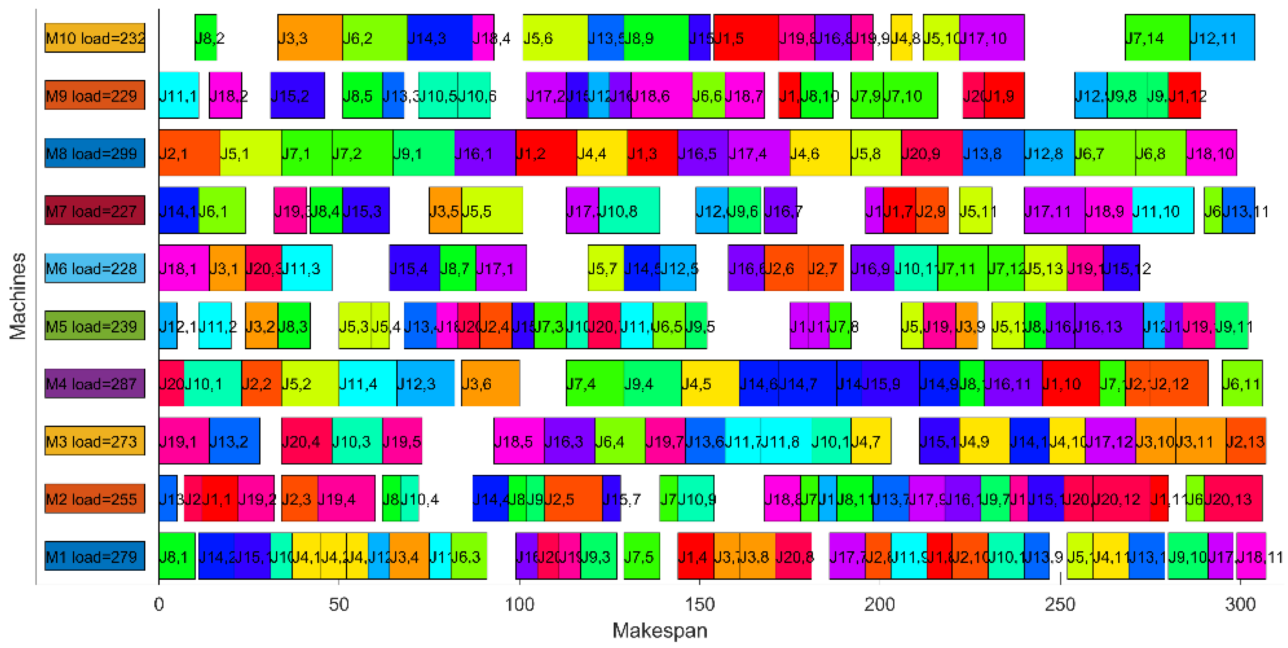
. The LB in the third column is provided by industrial solver DELMIA Quintiq [1]. It can be clearly seen that the proposed DIGWO obtains six lower bounds out of ten instances. According to the MRE metrics obtained by the algorithm, it is known that the proposed algorithm outperforms the other five compared algorithms in terms of solution accuracy. The T(AV) metric shows that the proposed algorithm also has the shortest average running time for all problems. Figure 23 shows the Gantt chart of the optimal results obtained by the proposed algorithm in MK09 (makespan = 307).

5.5.3. Comparison Results in Fdata

In this section, Fdata is used to test the performance of the proposed algorithm, and the results of the proposed DIGWO are compared with those of recent studies AIA, EPSO, MIIP and DOLGOA [31,55,67,68]. In order to eliminate randomness during the experiment, the results of 20 independent runs are shown in

Table 15. Comparison of DIGWO with other algorithms for Fdata.

Instance	n × m	LB	AIA a		EPSO b		MIIP c		DOLGOA d		DIGWO
			Best	Tcpu	Best	Tcpu	Best	Tcpu	Best	Tcpu	Best	WL	Avg	Tcpu
SFJS01	2 × 2	66	66	0.03	66	0	66	0	66	3.75	66	66	66	1.72
SFJS02	2 × 2	107	107	0.03	107	0	107	0.01	107	3.59	107	107	107	1.72
SFJS03	3 × 2	221	221	0.04	221	0	221	0.05	221	4.23	221	221	221	1.75
SFJS04	3 × 2	355	355	0.04	355	0	355	0.02	355	4.19	355	355	355	1.78
SFJS05	3 × 2	119	119	0.04	119	0	119	0.04	119	4.21	119	119	119	1.82
SFJS06	3 × 3	320	320	0.04	320	0	320	0.01	320	5.02	320	320	320	2.01
SFJS07	3 × 5	397	397	0.04	397	0	397	0	397	5.31	397	270	397	2.01
SFJS08	3 × 4	253	253	0.05	253	0	253	0.04	253	5.13	253	223	253	2.06
SFJS09	3 × 3	210	210	0.05	210	0	210	0.01	210	5.08	210	185	210	2.04
SFJS10	4 × 5	516	516	0.06	516	0	516	0.02	533	5.78	516	466	516	2.36
MFJS01	5 × 6	396	468	9.23	468	18.18	468	0.26	481	6.89	468	383	468	2.72
MFJS02	5 × 7	396	448	9.35	446	12.63	446	0.87	456	6.54	446	320	446	2.78
MFJS03	6 × 7	396	468	10.06	466	17.68	466	1.66	491	7.18	466	454	466	3.00
MFJS04	7 × 7	496	554	10.54	554	11.69	554	27.63	653	7.75	554	472	556.5	3.31
MFJS05	7 × 7	414	523	10.61	514	24.15	514	4.55	593	7.82	514	481	514	3.22
MFJS06	8 × 7	469	635	22.18	634	35.18	634	52.48	643	8.55	634	540	634	3.56
MFJS07	8 × 7	619	879	24.82	879	42	879	1890	1093	10.31	879	825	879.5	4.14
MFJS08	9 × 7	619	884	26.94	884	42.81	884	3600	997	11.13	884	800	885.1	4.52
MFJS09	11 × 8	764	1088	30.76	1059	38.61	1137	3600	1263	12.68	1055	305	1143	5.13
MFJS10	12 × 8	944	1267	30.94	1205	27.65	1251	3600	1517	13.68	1205	1125	1248.1	5.50
T(AV)			9.2925		13.529		638.8825		6.941			2.86
MRE			0.1422		0.1353		0.1428		0.2198			0.1350

^a CPU time on a 2.0 GHz processor in C++. ^b No system data provided by authors. ^c CPU time on a 2.83 GHz Xeon E5440 processor with 2 GB RAM in IBMILOG CPLEX 12.1 solver. ^d The CPU time on an Intel 2.90 GHz Core i5-9400F CPU in MATLAB 2019a.

. The LB in the third column is from the literature [69]. As can be seen in Table 15, the proposed DIGWO obtained 10 lower bounds in 20 instances. It is worth noting that MILP is an exact method, which means that the results obtained by the algorithm can be considered as the optimal solution. Compared with MILP, the proposed algorithm shows that the results of DIGWO in Fdata are always better than or equal to MILP. The results in the last two columns of Table 15 show that the proposed DIGWO is superior to the other four algorithms both in terms of solution accuracy and convergence speed.

5.6. Comparison Results in LSFJSP

In this section, 12 LSFJSP examples are used to further test the performance of the proposed DIGWO. The details of these examples are presented in Table 9. In order to verify the validity on LSFJSP of the proposed algorithm, the compared algorithms include WOA, Jaya, MFO, SSA, IPSO, HGWO and SLGA [21,27,58,59,61,65,70]. The first four algorithms are metaheuristics proposed in recent years, and the rest of the algorithms are studies about FJSP. In order to ensure that the experimental environment does not have special features, the algorithms listed above are run on the same device. The maximum number of iterations is set to 200. Each algorithm was repeatedly executed 10 times during the experiment, and makespan and critical machine load among them were recorded as evaluation criteria. The results obtained from the experiments are shown in

Table 16. Comparison of results in LSFJSP.

Instances	WOA		Jaya		MFO		SSA		IPSO		HGWO		SLGA		DIGWO
	Best	Avg	Best	Avg	Best	Avg	Best	Avg	Best	Avg	Best	Avg	Best	Avg	Best	Avg
YA01	1431	1505	1409	1502	1556	1599	1436	1490	997	1019	1156	1192	1210	1247	920	940
YA02	1473	1493	1474	1502	1534	1580	1741	1741	1016	1058	1205	1294	1230	1305	958	999
YA03	1740	1801	1732	1800	1910	1962	1672	1738	1154	1162	1451	1481	1324	1408	1052	1090
YA04	934	1105	986	1016	1054	1087	964	1007	672	690	761	780	825	864	642	659
YA05	1060	1113	1053	1093	1180	1225	1063	1113	737	758	911	945	856	893	666	687
YA06	1183	1216	1124	1205	1215	1250	1154	1204	781	821	961	975	851	900	660	693
YA07	1793	1884	1783	1838	1865	1951	1605	1700	1135	1152	1281	1306	1375	1423	1093	1133
YA08	1817	1931	1811	1872	2002	2073	1776	1818	1240	1261	1412	1469	1430	1484	1157	1179
YA09	1972	2054	1920	2049	2141	2233	1877	1944	1334	1352	1569	1631	1430	1481	1152	1198
YA10	2013	2093	2065	2117	2141	2212	1857	1919	1283	1313	1469	1530	1590	1613	1305	1346
YA11	2232	2336	2221	2276	2139	2241	1965	2057	1512	1530	1682	1731	1571	1624	1336	1374
YA12	2390	2549	2476	2557	2375	2466	2224	2312	1596	1644	1729	1758	1663	1708	1386	1426

and

Table 17. Comparison results of critical machine loads for the algorithm.

	WOA	SSA	MFO	JAYA	IPSO	HGWO	SLGA	HIGWO
YA01	1112	1112	1104	1013	833	953	942	816
YA02	1139	1372	1282	1161	887	1073	1066	808
YA03	1330	1366	1421	1270	1028	1393	1204	904
YA04	610	618	558	650	483	638	578	442
YA05	740	704	902	782	513	694	616	540
YA06	885	613	709	843	660	643	670	464
YA07	1308	1092	1137	1297	1018	1200	1168	947
YA08	1476	1449	1457	1472	1144	1403	1243	988
YA09	1490	1597	1685	1590	1210	1428	1267	976
YA10	1602	1613	1614	1443	1203	1399	1508	1136
YA11	1880	1694	1724	1838	1432	1654	1372	1174
YA12	2024	1461	1500	1980	1295	1470	1374	1158

, and the best convergence curves of each instance are shown in Figure 24, Figure 25, Figure 26 and Figure 27.

To analyze the data more intuitively, the best solutions of each problem in Table 16 and Table 17 are shown in bold font. From these data, it is evident that the proposed DIGWO obtains 11 optimal makespans out of 12 LSFJSP instances as well as the minimum critical machine load. Comparing the convergence curves of the algorithm, in most cases, DIGWO converges faster than other algorithms. Obviously, DIGWO is comparable to the makespan obtained by the metaheuristic algorithms involved in the comparison at 200 generations after updating to about 20 generations. The Friedman ranking of the compared algorithms on all problems is given in

Table 18. Average ranking of the comparison algorithm (Friedman), the level of significant α = 0.05.

Algorithm	Ranking	Final Priority
WOA	6.8333	7
Jaya	6.2500	6
MFO	7.5000	8
SSA	5.4167	5
IPSO	1.9167	2
HGWO	3.5000	3
SLGA	3.5000	3
DIGWO	1.0833	1
Test statistics	Friedman
p-value	4.0349 × 10−14

, and the results show that DIGWO is the best algorithm on all instances with p-value = 4.0349 × 10⁻¹⁴ < 0.05. From the information of the generated test examples, it is clear that the generated LSFJSP has not only low flexibility examples (F = 0.2, F = 0.3), but also high flexibility (F = 0.5). However, DIGWO always gives better results on these problems.

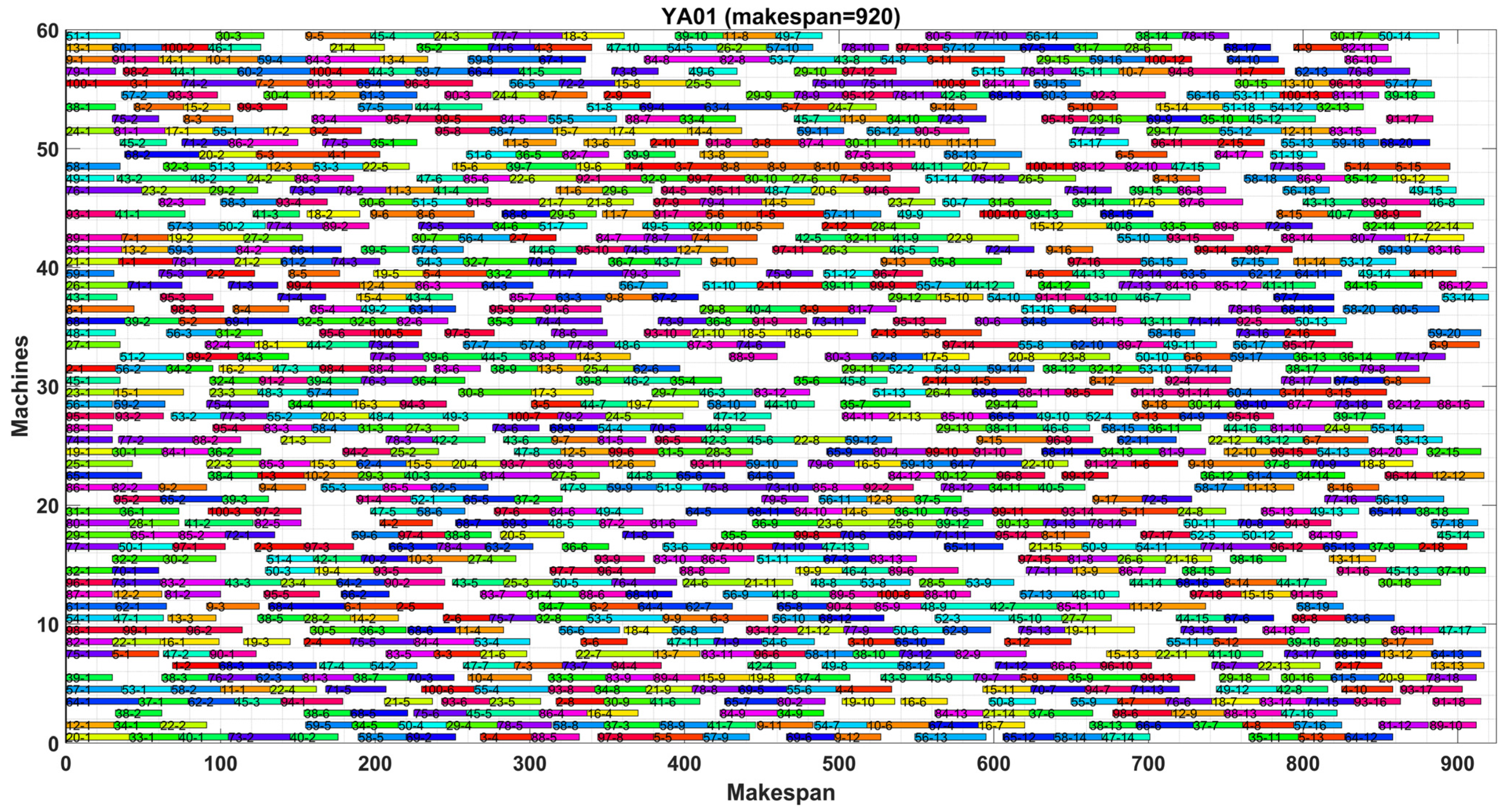
Figure 28 shows the optimal makespan Gantt chart obtained by the proposed DIGWO in YA01. The operations are denoted by “Job-operation”, and because of the large number of machines, the vertical coordinates are not annotated machine sequentially, and the horizontal coordinates in the figure indicate the processing time period of the operation. From the graph, it can be observed that the majority of machines were started for processing at the moment 0. In addition, no machine is found to be idle for a long time or overused, which is in line with the concept of smart manufacturing and effectively saving process time costs.

By the above comparison, the characteristics of FJSP and the idea of GWO are combined, and the discrete update mechanism of DIGWO algorithm is designed, so that each grey wolf individual of GWO has simple intelligence. The success of the DIGWO design lies in the effective initialization strategy as well as the DGUO strategy, which not only ensures the quality of the initial population, but also enhances the efficiency of the search in the process of iterative update. For FJSP, the proposed algorithm has better convergence compared to the original GWO. In conclusion, DIGWO has the inherent ability to solve LSFJSP, and the proposed DIGWO is generalizable and can be applied to FJSPs of different scales.

6. Conclusions

We propose a discretized improved grey wolf optimization algorithm to solve FJSP with the objectives of minimizing makespan and critical machine load. The GWO algorithm has the advantage of few parameters and easy implementation; however, it may converge prematurely. For this purpose, several improvement strategies are designed to enhance the search capability of the algorithm for FJSP. The effectiveness of the algorithm is verified through extensive comparison experiments with the algorithms proposed in the literature published in recent years. The experimental and comparative results show that the algorithm can obtain the most well-known solutions to most problems. The main advantages of the DIGWO algorithm proposed in this paper are as follows. (1) The proposed initialization strategy is introduced to improve the quality of the solution. (2) The discrete update mechanism is designed to ensure that the algorithm can be effectively applied to solve the problem, while being more competitive compared to recent research on FJSP by GWO. (3) The proposed adaptive convergence factor enhances the global search capability of the algorithm.

In recent years, carbon emissions and energy consumption have been hot topics in modern manufacturing, and will therefore be considered for future research directions. Additionally, some uncertainties such as machine failures and workpiece insertion are also the focus of our research.